Approximation and elections

(1)

RIT Scholar Works

Theses

Thesis/Dissertation Collections

2007

Approximation and elections

Eric Brelsford

Follow this and additional works at:

http://scholarworks.rit.edu/theses

This Thesis is brought to you for free and open access by the Thesis/Dissertation Collections at RIT Scholar Works. It has been accepted for inclusion in Theses by an authorized administrator of RIT Scholar Works. For more information, please [email protected].

Recommended Citation

(2)

Approximation and Elections

Eric Brelsford

Computer Science Department Rochester Institute of Technology

(3)

(4)

Contents

1 Introduction 7

1.1 Overview . . . 8

1.2 Tips for Reading . . . 9

1.3 Acknowledgments . . . 10

2 Social Choice Theory 11 2.1 Voting Systems . . . 11

2.1.1 Scoring Protocols . . . 12

2.1.2 Other Voting Systems . . . 13

2.2 Criteria in Social Choice Theory . . . 16

2.3 Impossibility . . . 17

2.3.1 Arrow’s Theorem . . . 17

2.3.2 Gibbard-Satterthwaite Theorem . . . 18

3 Computational Social Choice 19 3.1 Definitions and Notation . . . 19

3.1.1 Instance Encoding . . . 20

3.2 Control . . . 20

3.2.1 Definitions . . . 21

3.2.2 Results . . . 24

3.3 Manipulation . . . 24

3.3.1 Definition . . . 24

3.3.2 Results . . . 25

3.3.3 Approximability . . . 26

3.4 Bribery . . . 27

3.4.1 Definitions . . . 27

3.4.2 Results . . . 27

3.4.3 Approximability . . . 28

3.5 Other Problems . . . 28

(5)

3.6 Average-Case Elections . . . 28

3.6.1 Voter Preferences . . . 29

3.6.2 Prices and Weights . . . 30

4 Approximation Algorithms 31 4.1 NP Optimization . . . 31

4.2 Approximation . . . 32

4.2.1 Notation . . . 32

4.2.2 APX . . . 33

4.2.3 PTAS and FPTAS . . . 34

4.2.4 Other Measures of Approximation . . . 35

4.3 Some Results Regarding Approximation . . . 36

4.3.1 Strong NP-hardness and Pseudo-Polynomial Time . . 36

4.3.2 p-simpleness . . . 37

4.3.3 Other Approximation Results . . . 37

4.4 Creating Approximation Algorithms . . . 37

4.4.1 From Pseudo-Polynomial Time Algorithm to FPTAS . 38 5 Approximating Bribery 39 5.1 Optimizing Bribery . . . 39

5.2 A General Result . . . 40

5.3 Manipulation and Bribery . . . 40

5.4 Approximation, Unpriced to Priced . . . 41

6 The Knapsack Problem 45 6.1 Similarity Between Plurality Bribery and the Knapsack Prob-lem . . . 45

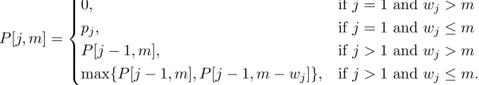
6.2 The Binary Knapsack Problem . . . 46

6.2.1 KP Optimization . . . 48

6.2.2 Other Modifications of Binary KP . . . 49

6.3 Algorithms for the Knapsack Problem . . . 53

6.3.1 The Dynamic Programming Algorithm . . . 53

6.4 Approximation Algorithms for KP . . . 54

6.4.1 KP . . . 54

6.4.2 MinKP . . . 55

7 plurality-weighted-$bribery 57 7.1 Optimal Algorithms . . . 57

7.2 Plurality Negative Bribery . . . 59

(6)

CONTENTS 5

7.4 Attempted approximations . . . 63

7.4.1 Modifying Existing, Optimal Algorithms . . . 63

7.4.2 Greedy Heuristics . . . 64

8 Approximating Control 67 8.1 Adding Candidates . . . 67

8.1.1 Weighted Cases . . . 68

8.2 Deleting Candidates . . . 79

8.3 Partitioning . . . 80

8.4 Adding and Deleting Voters . . . 81

(7)

(8)

Chapter 1

Introduction

Any culture that requires that a decision be made within a group neces-sarily creates methods for aggregating each individual’s preferences. For instance, we see such a need in political elections, committees, and busi-nesses. With the Internet and the increasing use of multiagent software systems, the general need for means of aggregating differing preferences has increased dramatically.

Voting is one way to come to a single option (or small group of options) out of a larger pool of candidate options. Many voting systems exist, and criteria exist (within the field of social choice theory) for deciding which most fairly and accurately take into account the preferences of each voter.

Since there is generally much to be gained from influencing such a vote through manipulation or bribery, one desirable criterion of fairness would be whether such activities are impossible in the system. However, it has been shown that a reasonable system that disallows manipulation does not exist [18, 43], so the next-best solution would be a system in which deciding how to bribe or otherwise influence the vote is so computationally difficult as to render it impossible or highly unlikely.

While the debate over which voting systems are most fair and effective is on record of existing over the past few centuries (and likely goes further back to ancient Greece), there may exist the seeds of a renewal of this debate in the current boom in voting due to new technologies. For one, in artificial intelligence agents may vote to determine the best course of action to take given the individual’s preferences. In addition, algorithms in search engines and meta-search engines do order results in a manner that assumes a ranking was somehow approached. Voting is not only on the rise in software, of course, as most any user of the Internet could demonstrate. Internet users

(9)

routinely vote most any user of the Internet could demonstrate. Internet users routinely vote online in situations ranging from the inane (e.g., rating a video on YouTube) to the potentially crucial (e.g., voting on whether a story is newsworthy or not on any of a plethora of such sites, including Digg, Reddit, and Newsvine).

These newer uses of voting systems are interesting. They are used in environments where there are potentially far more candidates and voters than are conventionally seen in, say, political elections. Also, in these new environments, voting and manipulation can be automated to some degree, thus making the possibility of manipulation and control even more real than it has been in the past.

Faliszewski, Hemaspaandra, and Hemaspaandra have proved for a num-ber of voting systems that the brinum-bery problem is too complex to be feasible (i.e., NP-complete) [15], and much research has been put forth determining the complexity of other problems related to voting.

But it is still possible in the optimization cases of these problems that there exist approximation algorithms that can find a good solution with a reasonable amount of computation. That is, while a voting system may seem “resistant” to a particular form of manipulation as described by previous research, it may be that the problem is not as difficult if we allow a constant amount of error. Or, it may be that the problem is still difficult when error is allowed, thus making the voting system even more resilient with respect to some forms of manipulation. This thesis will examine the possibility of such approximations for some problems in elections.

1.1

Overview

We will start with some background on traditional social choice theory, in-cluding definitions of voting systems and criteria by which these systems are judged (Chapter 2). This background along with a small amount of computer science theory will be sufficient for the next chapter,Chapter 3, which will sketch the current state of the field of computational social choice. Some of the more relevant problems that are often studied under the um-brella of elections and voting systems will be defined. In addition, the known complexity of the problems will be summarized for some voting systems.

Next we will veer more towards theoretical computer science in

Chap-ter 4, an exploration of approximation algorithms. This chapter contains

(10)

1.2. TIPS FOR READING 9

later chapters mention an approximation concept, as opposed to being read through on its own.

Once this background is covered, the chapters containing original results begin.

First, we find some general approximation results on the problem of bribery in voting systems inChapter 5. These proofs rely on the complexity of manipulation problems for the same voting systems.

Next, we attempt to show the approximability of a specific bribery prob-lem, known as plurality-weighted-$bribery. This takes part in a few chapters. The first chapter regarding this problem isChapter 6, which deals with the knapsack problem, a classic and simply stated combinatorial problem. This chapter will consist of a number of definitions as well as an overview of some generalizations of the problem and approaches that have been taken towards solving them. The motivation behind studying the knapsack prob-lem is the potential relation between it and the bribery probprob-lem at hand that could be exploited. The knapsack problem could also prove to be use-ful regarding other problems in the realm of computational social choice, and we hope that this chapter might draw some connections between the two realms that have not been previously exploited.

Given this, inChapter 7, we will take a look at the approximability of the bribery problem plurality-weighted-$bribery. While we do not directly prove approximability results for this problem, we do prove that a special case of the problem is not approximable.

Finally, Chapter 8 contains an analysis of the approximation of some control problems. For some problems we can prove that they are at least partially resistant to being approximated, while other problems are far more resistant.

1.2

Tips for Reading

A minimal knowledge of computational complexity theory will be assumed throughout this work. An understanding of the complexity classes P and NP as well as the concept of NP-completeness will be essential at points. Any textbook regarding algorithms or complexity theory will likely have an adequate review of these principles. Garey and Johnson’s canonical book [17] can also provide this background.

(11)

• Sections 5.2 and 5.4 contain general results regarding the approxima-bility of bribery,

• Sections 7.2 and 7.3 contain our results pertaining to bribery in elec-tions using the plurality voting scheme, and

• Section 8.1 holds our non-trivial proofs of the nonapproximability of control by adding candidates to plurality elections.

Some of the proofs (especially those in Chapter 8) are especially tedious. It is advisable to read the proofs in Chapter 5 first, as those follow the same pattern and are far simpler.

1.3

Acknowledgments

I would like to thank my advisor, Edith Hemaspaandra, for all of her guid-ance and suggestions. Piotr Faliszewski was also extremely helpful, namely by making a number of corrections and helping me clarify some points in this thesis.

(12)

Chapter 2

Social Choice Theory

Social choice theory is an area of research with close ties to political science and economics that studies methods for selecting some options out of many by aggregating the preferences of a number of people or agents. This might include voting on a leader out of a number of candidates, deciding whether a proposal should become law, or settling an argument over what to make for lunch.

In particular, work in the area generally attempts to decide which voting system is most fair for a particular task. In this capacity, the beginning of social choice theory is usually dated as the late eighteenth century in France1_, when Borda and Condorcet had a disagreement over which voting system should be used in the French Academy of Sciences [42]. Both parties in the argument were mathematicians, and mathematics, including computer science, has continued to be a strong force in the field since its inception.

As software has become more complex and pervasive, concepts from so-cial choice have progressed beyond describing methods of collective decision making in societies. Some computer systems also use these voting systems in order to decide which course of action is best, much as societies do, and this has contributed to an increased interest in the field.

2.1

Voting Systems

What follows is a discussion of some of the more well-known voting systems. A voting system takes a set of voters with preferences over some set of candidates and determines a set of winners. We will assume that preferences

1_{Although, recently, it has become clear that the theory has been studied as early as}

the thirteenth and fifteenth centuries by Llull and Curanus[20]

(13)

over candidates are strict, that is, a voter is not allowed to be indifferent between two candidates, and we will represent a voter’s or a group of voters’ preferences by listing them in order of most- to least-preferred. For example, a voter preferring candidatecto ato b would be represented by c > a > b.

An election, E, is then represented as a pair of sets, (C, V), whereC is the set of candidates andV is the set of voters.

2.1.1 Scoring Protocols

Scoring protocols are generally straightforward: a list of points (often called a scoring vector, α = (α1, α2, . . . , αm)) to be assigned to the candidates in

the election according to their position in each voter’s preferences is defined by the protocol. That is, a voter has preferences c1 > c2 > . . . > cm, and

for 1≤i≤m assigns αi points to candidateci. Those candidates with the

most points win the election.

Example 2.1.1. Consider a scoring protocol over3candidates with scoring

vector (5,4,3). If these candidates are {c1, c2, c3} and a voter most prefers

c3, c1 next, and c2 least (i.e., c3> c1> c2), then the voter gives5 points to

c3, 4 toc1, and 3 to c2.

plurality

Also known as simple majority or first-past-the-post, this is the most com-mon voting system used in politics today. Part of its popularity is certainly due to its simplicity: the candidate(s) with the largest number of votes is the winner, where the candidate receives a vote whenever it is most preferred by a voter.

Plurality is a family of scoring protocols with scoring vector (1,0, . . . ,0), that is, a voter’s most preferred voter gets a point, no other candidates get any points from the voter. Due to the simplicity of the scoring vector, in practical use one rarely thinks of plurality as a scoring protocol, but rather of a vote that gives one point to the most-preferred candidate.

Borda count

Each voter’s most-desired candidate gets |C| −1 points, the second most-desired candidates get |C| −2 points, etc., where |C|is the number of can-didates in the election. More formally, the scoring vector is (|C| −1,|C| −

(14)

2.1. VOTING SYSTEMS 13

This method is appealing over plurality because voters are able to give their opinions of all of the candidates (as opposed to just their favorite one) and the degree of separation between candidates in a ranking is kept track of (in addition to their ordering). For a more in-depth yet very accessible discussion on the relative merits of Condorcet’s (below) and Borda’s counts, see [42].

veto

A voter gives one point to each candidate except for the one it least prefers, which gets zero points. That is, the scoring vector (1,1, . . . ,1,0) is applied to each voter’s preferences.

2.1.2 Other Voting Systems

While scoring protocols are among the simplest useful voting systems to define, there are many other voting systems, some of which are used in practical settings. What follows is a mere sampling of these systems, some of which are looked at in more depth in later chapters.

single transferable vote

Single transferable vote (STV) takes place in a number of rounds. During each round, the candidate with the least votes (as judged in a plurality election; ties are handled differently in separate versions) is eliminated, and all voters who were voting for this candidate vote for their next preferred candidate in the next round.

Example 2.1.2. Consider the election described by the following voters and

their preferences:

Voters With Preferences 4 x > y > z

3 z > y > x

2 y > z > x

(15)

If the election has more candidates, the process is identical, but there are more rounds where candidates are eliminated until the desired number of winners is found.

Single transferable vote is used in some regions from the local to federal levels, perhaps most notably in Australia.

Condorcet voting

Under Condorcet voting, the candidate who strictly beats each other candi-date in a pairwise contest wins overall.

Example 2.1.3. Say we had the following election:

2 z > y > x

2 y > z > x

then, overall, the voters prefery tox (four points to three), ztox(also four points to three), and y to z (five points to two). Since y beats both x and

z (all of the other candidates) when it goes up against them individually, y

would be the Condorcet winner.

Such a criterion for a fair election seems a common-sense choice, however, there will not always be a Condorcet winner due to cycles in preferences. This is often called Condorcet’s Paradox.

Example 2.1.4. To see how the paradox appears, consider the following

election over three candidates,x, y, and z:

3 y > z > x

3 z > x > y

There is no Condorcet winner in the above election. To see this, we first compare candidates x and y, and we see that six voters prefer x and three voters would rather y. Then, when comparing y and z, six voters prefer y

and threez. So far, it looks as thoughx should be the winner of the election since it beatybetween the two andybeatz. However, we have yet to compare

x and z, and, when we do, we are chagrined to find that six voters prefer z

and threex. That is, the group of voters has decided that its preferences are

(16)

2.1. VOTING SYSTEMS 15

Dodgson voting

Dodgson voting is an attempt to sidestep the Condorcet paradox by mak-ing the candidate who is closest to bemak-ing a Condorcet winner the winner. Determining which candidate is the closest consists of counting the number of switches that would need to be made in the voters’ preferences in order to make the candidate a Condorcet winner. Then, the candidates who have the smallest value for this number is the Dodgson winner.

A “switch” in this context is changing a voter’s preferences by flipping two adjacent candidates in the preferences. For example, changing a voter’s preferences from z > x > w > y to z > x > y > w would count as one switch.

This voting system is named after its creator, the mathematician Charles Dodgson, who is better known by his pseudonym Lewis Carroll.

approval voting

In this system, each voter gives a point to each candidate he or she approves of, and a candidate with the highest number of points wins.

Example 2.1.5. There might be an election over candidates (v, w, x, y, z)

with the following voters:

Voters With Preferences 2 (1,0,0,1,1) 2 (1,1,1,1,0) 2 (0,1,0,0,1) 1 (0,0,1,0,1)

That is, there are two voter who vote with preferences (1,0,0,1,1), meaning that they approve of candidates v, y, and z, but not w or x. Here z wins with five points—five voters approve of candidate Z.

At times, k-approval voting, where a voter must approve of exactly k

candidates, or other situations, such as whenk is half the number of candi-dates, are examined.

maximin

(17)

2.2

Criteria in Social Choice Theory

Much research has been devoted to finding voting systems which are fair. Generally, we consider a fair election to be one in which the will of the voters is reasonably expressed. There are a number of criteria that a fair election scheme could consist of, and here are a few concrete ones:

Pareto condition

A voting system satisfies the Pareto condition if, when candidate x is pre-ferred by all voters over candidate y, candidate x will be preferred over candidateyoverall, as measured by the voting system. One modification of this condition is to make it weak by saying thatxmust be strictly preferred toyin each voter’s preferences (i.e., no indifference is allowed in preferences betweenxand y). Similarly, the condition can be made strong by stipulat-ing that only one voter need strictly preferx to y, while the rest may find

xat least as good as y.

monotonicity

If a voting system never ranks a candidate lower because some voters rank the candidate higher than before, the voting system is said to obey mono-tonicity.

Many voting systems do obey this criterion. The voting systems that are not monotone are often those which take place in rounds. One such voting system is single transferable vote.

independence of irrelevant alternatives

This condition (in [2]) states that if candidatexis preferred over candidatey

overall, and one or more voters change their preferences regarding candidates other thanxand y,x should still be preferred toy overall.

While this condition seems to be a desirable one, many voting systems do not obey it.

Example 2.2.1. Consider a Borda election like this:

Voters With Preferences 2 w > x > y > z

(18)

2.3. IMPOSSIBILITY 17

Clearly, the voters preferxoverzwith scores7and6, respectively. However, say we modify the preferences of both of the voters from the first set from

w > x > y > z to w > y > x > z. Now, even though the voters changed their minds by promoting y, the overall preferences now favor z over x with scores6and5. Althoughyis not relevant to the relative rankings ofxandz, the ranking of y does have an effect on which of the two is preferred overall.

non-dictatorial

We should certainly expect a voting system to not give one voter the ability to sway the outcome of the election. Otherwise, if a single voter ultimately decides the outcome of an election, the scheme isdictatorial. That is, if some voter,d, most prefers candidatexin an election andx wins no matter what the rest of the voters prefer, then the voting system being used is dictatorial, but if there is no such d, then the system is non-dictatorial.

2.3

Impossibility

Some of the work in social choice theory more relevant to this thesis includes impossibility results, that is, proofs that particular properties cannot exist, or that certain sets of properties cannot coexist, in voting systems.

2.3.1 Arrow’s Theorem

This theorem, which was discovered by the economist and Nobel Prize win-ner Kenneth Arrow, attempts to determine whether a “fair” voting system can exist. It states that a voting system over three or more candidates cannot at the same time

• obey monotonicity,

• obey independence of irrelevant alternatives,

• ensure that any possibility out of the candidates could be selected, and

• be non-dictatorial,

(19)

One formulation and proof of this is in [2], though it has since been made stronger (e.g., by weakening some of the above conditions) and its proof has been simplified [40].

2.3.2 Gibbard-Satterthwaite Theorem

This theorem, found independently by Gibbard and Satterthwaite, is sim-ilar to Arrow’s. It states [18, 43] that a voting system over three or more preferences cannot at the same time

• ensure that any possibility out of the candidates could be selected,

• be immune to manipulation, and

• be non-dictatorial.

Manipulation in the context of voting systems occurs when a voter or set of voters are better off not voting with their true preferences and, so, choose to vote strategically in order to gain a better outcome. That is, the manipulating voters will see a more preferred candidate win by voting with preferences that differ from their actual ones. Certainly it is desirable to use a voting system that is not manipulable, since a voting system does not feel fair or effective if it does not make voters feel comfortable with expressing their true preferences because other voters might be manipulating the election.

In [40], Reny looks at the relationship between Arrow’s and the Gibbard-Satterthwaite theorem in more detail. In fact, the author uses what is essentially the same, relatively simple proof to show both theorems hold.

As this theorem shows that manipulation will always be a possibility when more than three candidates are involved in a reasonable voting sys-tem, it motivates the current research into the computational complexity of performing this manipulation and of computational social choice in general. Such research can give us a better idea of how susceptible a system is to manipulation (since we know that essentially all are susceptible) or some related problem and in some ways this research can tell us which systems are better than others.

(20)

Chapter 3

Computational Social Choice

Whereas social choice theory is interested in the existence of voting systems with particular properties (Chapter 2), computational politics, or computa-tional social choice, is an attempt to determine the computacomputa-tional difficulty of problems dealing with particular aspects of voting systems.

Similarly to social choice theory, a good deal of focus has been spent on finding the complexity of performing possibly mischievous actions on an election in a given voting system. The key difference is that computational social choice can in some instances reveal that, while, yes, this form of manipulation ispossible in such-and-such voting system, finding the way to do so is NP-complete and therefore can generally be considered intractable. In this way, computational social choice can give us a better characterized picture of which voting systems are vulnerable to certain bad occurrences.

In addition to these somewhat negative problems, effort has been put into determining the complexity of certain positive problems, such as determining the winner of an election or the scores of candidates in an election. Perhaps surprisingly, for some voting systems these problems are rather difficult. In fact, some are unlikely to be in NP1_.

3.1

Definitions and Notation

Before we get into the definitions of the various problems to be considered, we should define the notation to be used.

An election is a tuple (C, V) over a set C of candidates and a multiset

V of voters. Each v ∈V has a list of preferences over all candidates in C,

1_{See, for example [22], where winner determination for Dodgson voting is shown to be}

complete for parallel access to NP

(21)

prefs=c1 > c2 > . . . > cn where c1 is more preferred byv to c2, etc. If an election isweighted, eachvmust also have a non-negative integer weight,ω. Given an election (C, V) and a candidate c ∈ C, we will denote c’s score in the election (if the election is taking place in a voting system that assigns scores to candidates, as will always be the case in this thesis) as

score₍C,V)(c), and the value of this score is as defined by the voting system at hand, which should be clear from context. In many cases, depending on the voting system, a winner of (C, V) is any c∈C such that score₍C,V)(c) is the largest score in (C, V). As a set of candidates can win an election, we will sometimes look for aunique winner, one which is the sole winner of an election.

3.1.1 Instance Encoding

For any problem in this area, we will assume that the instances are encoded reasonably and that each voter and its preferences are an entry in the in-stance, much like a ballot in an election. In some cases, we will instead look atsuccinct elections, where one entry may represent multiple, identical voters.

For instance, if there arekvoters with identical preferences (and weights, if weights may vary), then each must be separately represented in a non-succinct election, that is, there arekdistinct entries in the election. On the other hand, the same k voters would be represented in a succinct election as a single entry, but with the frequency countk.

While this may seem to be a small difference, succinctness can have an impact on the complexity of problems dealing with elections. This is so because complexity is measured as a function of the length of the input, and input length for succinct elections can be significantly smaller than in the non-succinct case. We will encounter this in some detail in Section 7.2.

3.2

Control

The study of control in elections deals with the possibility of affecting the outcome of elections by changing the structure or makeup of the election. This involves a chairperson in charge of the election adding or removing voters or candidates, or partitioning voters or candidates into subelections that precede the main election.

(22)

3.2. CONTROL 21

control is used when trying to make a certain candidate lose an election. In either case, traditionally in control a candidate wins an election only if it is the unique winner, that is, there are no ties allowed. Therefore, when we are trying to make a particular candidate lose the election, it is sufficient to make some other candidate tie the given candidate in order to make it lose. The complexity of a number of control problems have been studied in some depth. In [5], Bartholdi, Tovey, and Trick initiate the research of con-trol by looking at the complexity and possibility of constructively concon-trolling elections under the plurality and Condorcet voting schemes.

The destructive case was studied by Hemaspaandra, Hemaspaandra, and Rothe in [21], for the plurality, Condorcet, and approval voting. The authors also performed the analysis for approval in the constructive cases, since [5] did not deal with approval.

Please refer to Chapter 2 for background on the voting systems men-tioned. As the definitions and results of the aforementioned papers will be used in Chapter 8, let us present them here.

3.2.1 Definitions

Control problems largely include adding or deleting candidates or voters or partitioning candidates or voters in order to make a particular candidate win or lose the election. The problems are defined identically for each vot-ing scheme (with the exception that in the case of approval votvot-ing, a voter’s list of preferences is a 0-1 vector the size of the set of all potential candidates as opposed to an ordered list of candidates), and the constructive versus de-structive cases are similar enough that we can collapse them into the same definition. The constructive case of each question will be stated with the modifications for the destructive case in brackets. Nothing changes between the two cases within the “Given” field of the problems. The following defi-nitions are adapted from [5, 21].

Adding Candidates

Given: A setCof qualified candidates and a distinguished candidatec∈C,

a set D of possible spoiler candidates, and a set V of voters with preferences over C∪D.

Question: Is there some subset of D whose entry into the election would

(23)

In this case, the voters’ preference lists are assumed to be over all po-tential candidates. That is, all candidates who might be up for election, including those inD, are considered.

Deleting Candidates

Given: A set C of candidates, a distinguished candidate c∈C, a set V of

voters, and k∈Z+ _with_k_{≤ |}_C_|_.

Question: Is there some subset of k or fewer candidates in C [C − {c}]

whose disqualification would assure that cis [not] the unique winner?

Partitioning Candidates

When partitioning candidates, there are two intuitive ways that candidates from either segment of the partition might compete:

• winners are determined from within the first segment defined by the partition that go on to compete with all of the candidates in the second segment defined by the partition, or

• winners from both segments are found and compete in a run-off elec-tion.

In either case, an instance of the problem is the same:

Given: A set C of candidates, a distinguished candidate c∈ C, and a set

V of voters.

The question for the first case, Control by Partition of Candidates is:

Question: Is there a partition ofCintoC1 andC2such thatcis the unique winner in the sequential two-stage election in which the winners in the subelection (C1, V) who survive the tie-handling rule move forward to face the candidates in C2 (also with the voter setV)?

The question for the second case,Control by Run-Off Partition of Can-didates is:

Question: Is there a partition of C into C1 and C2 such that c is the

(24)

3.2. CONTROL 23

In any partition, as described by [21], there are two tie-handling rules:

• TE, “ties eliminate,” where candidates that tie during subelections do not move on to the next round, and

• TP, “ties promote,” where candidates that tie during subelections do move on to the next round.

As is clear in Table 3.1, tie-handling rules do sometimes affect the complexity of the partition control, depending on the voting system.

Adding Voters

Given: A set C of candidates, a distinguished candidate c ∈ C, a set V

of registered voters, a set W of unregistered voters, andk∈Z+ _with

k≤ |W|. All voters have preferences over the entire set C.

Question: Is there a set ofkor fewer voters inW whose registration would

assure that c is [not] the unique winner?

Deleting Voters

Given: A setCof candidates, a distinguished candidatec∈C, andk∈Z+

withk≤ |V|.

Question: Is there a set of k or fewer voters in V whose deletion would

assure that c is [not] the unique winner?

Partitioning Voters

Given: A set C of candidates, a distinguished candidate c∈C, and a set

V of voters.

Question: Is there a partition ofV intoV1 andV2 such thatcis the unique winner in the hierarchical two-stage election in which the survivors of (C, V1) and (C, V2) run against each other with voter set V?

(25)

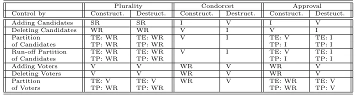
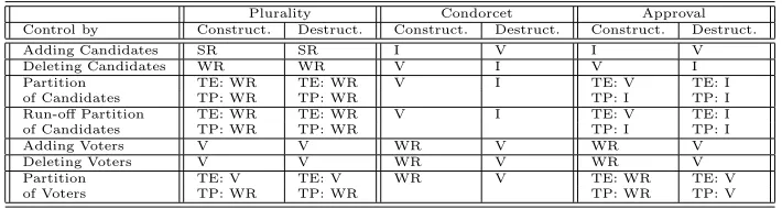
Plurality Condorcet Approval Control by Construct. Destruct. Construct. Destruct. Construct. Destruct.

Adding Candidates R R I V I V

Deleting Candidates R R V I V I

Partition TE: R TE: R V I TE: V TE: I of Candidates TP: R TP: R TP: I TP: I Run-off Partition TE: R TE: R V I TE: V TE: I of Candidates TP: R TP: R TP: I TP: I

Adding Voters V V R V R V

Deleting Voters V V R V R V

Partition TE: V TE: V R V TE: R TE: V

[image:25.612.154.508.77.172.2]

of Voters TP: R TP: R TP: R TP: V

Table 3.1: ([21]): Summary of results regarding the complexity of control prob-lems for plurality, Condorcet and approval voting schemes as presented in [21]. Constructive results for plurality (except for TE and TP for Partition of Voters) and Condorcet via [5], the rest are from [21]. I = immune, R = resistant, V = vulnerable, TE = Ties-Eliminate, TP = Ties-Promote.

3.2.2 Results

Table 3.1 presents the results regarding the computational complexity of the voting systems Plurality, Condorcet, and Approval. The results label each system asimmune,resistant, orvulnerable to the given form of control. If a system is immune to a particular type of control, it is impossible to perform that control on an election in the system—that is, the preferred outcome cannot be attained by performing the respective control technique. If such control is possible, in these cases computing it is NP-hard (resistant) or in P (vulnerable).

Since the immune and vulnerable control problems are in P and are thus easily optimizable, we will be more interested in those which are proven resistant. In Chapter 8 we examine the approximability of those control problems which are resistant.

3.3

Manipulation

Manipulation is generally the problem of voters voting with dishonest pref-erences for their own benefit. Like control, this problem has been studied under numerous voting systems, in both constructive and destructive situa-tions, and with a few variasitua-tions, such as where the voters are weighted.

3.3.1 Definition

(26)

3.3. MANIPULATION 25

E-manipulation

Given: A set C of candidates, a set V of voters, a set S of potential

ma-nipulative voters such that V ∩S =∅, and a distinguished candidate,

p.

Question: Is there a setting of the preference lists of the voters inS such

that pis a winner of election (C, V ∪S) under voting system E?

Note that, in contrast to the above definitions of control problems, we here attempt to make pa winner, but not necessarily the sole winner, of the election.

This is for the constructive case, where the manipulators try to makep

win the election. In the destructive case, the problem is defined identically, with the difference that the manipulators attempt to make p lose. For the weighted cases, everything is exactly the same except, of course, the voters have weights.

3.3.2 Results

The study of the complexity of manipulation was initialized for the un-weighted case was determined for some voting systems by Bartholdi, Tovey, and Trick [26].

In [13], Conitzer, Lang, and Sandholm look at how many candidates it takes for manipulation to become NP-complete for various voting systems in the weighted case, and, in doing so, produce a more complete picture of the complexity of manipulation. In the constructive case, manipulation becomes NP-complete for many systems rather quickly if the votes are weighted, as shown in Table 3.2. In the destructive case, the problem remains in P for many of the systems analyzed, though they did find that it was NP-complete for STV and plurality with a runoff.

(27)

Number of candidates 2 3 ≥4

Borda P NP-complete NP-complete Veto P NP-complete NP-complete

STV P NP-complete NP-complete

plurality with runoff P NP-complete NP-complete

maximin P P NP-complete

[image:27.612.198.464.77.168.2]

plurality P P P

Table 3.2: ([13]): The computational complexity of weighted manipulation for relevant voting systems with the given number of candidates (2, 3, or≥4) in the election. Excerpted from results originally presented in [13].

In [23] Hemaspaandra and Hemaspaandra present some dichotomy the-orems regarding the complexity of manipulation for scoring protocols. We will restate the main result of this paper here for the reader’s convenience (modified only to keep notation consistent).[23]

Theorem 3.3.1([23], Theorem 2.1). For eachm and each scoring protocol

α= (α1,· · ·, αm), α-weighted-manipulation is in P if α2 =α3 =· · ·=αm,

and isNP-complete otherwise.

3.3.3 Approximability

The optimization of manipulation is tricky to define. Clearly, we want to minimize the number of voters that we manipulate in order to make the preferred candidate win the election.

Do we say that when optimizing manipulation we only leave in the elec-tion those voters for whom we have changed the preference lists? In this case, the voters left out are also acting in a manipulative fashion by abstain-ing. That is, there is little gained by the manipulators, who presumably would like to minimize their chances of being detected, since they all would be doing something manipulative.

(28)

3.4. BRIBERY 27

As we have been unable to find a suitable definition of optimal manipu-lation, we will not examine the approximability of manipumanipu-lation, which by its nature demands an optimization problem.

3.4

Bribery

Bribery is a natural extension of manipulation and a natural problem in the realm of voting systems.

3.4.1 Definitions

E-bribery

Given: A setC of candidates, a setV of voters, a distinguished candidate

c, and a positive integer k, the budget.

Question: Is there a set of at most k voters whose preferences can be

changed to make c the winner of election (C, V) under systemE?

This is the simplest version of bribery, where each voter’s price and weight are the unit price and weight, assumed to be 1. It is also interesting to look at problems where the weights (ω ∈ Z+_{) vary by voter, the prices}

(π ∈ N_{) of the voters vary, or both vary independently. These problems}

are referred to as E-weighted-bribery, E-$bribery, andE-weighted-$bribery, respectively.

3.4.2 Results

The study of bribery from a computational complexity point of view was initiated in [15], by Faliszewski, Hemaspaandra, and Hemaspaandra. They find the complexity of bribery for each of the variations mentioned above, and for a number of voting systems. One interesting result of this exam-ination is that plurality voting with weighted votes and varying prices is NP-complete for as few as two candidates (the approximability of which is studied in Chapter 7), whereas bribery in plurality voting with only one of those qualifications is in P. However, for the case where the votes are weighted and the prices vary, if either the weights or prices are encoded in unary, the problem comes back down to P.

(29)

Finally, [15] also provides a look at the relationship between bribery and manipulation, the latter of which has been studied previously and rather thoroughly. In the authors’ words, “bribery can be viewed as manipulation where the set of manipulators is not fixed in advance and where deciding who to manipulate is a part of the challenge.” Of course, part of this challenge is that each voter might have weights or prices that vary. In addition, it is shown that any manipulation problem is many-one reducible to the equivalent $bribery problem, so some of the known manipulation results immediately give hardness results for equivalent bribery problems.

3.4.3 Approximability

Since these bribery problems are quite new, approximation in this context has not yet been studied. In Chapter 5 we initiate this study and look at the possibility of approximating bribery in general. Then, in Chapter 7, we examine the approximability of bribery in the plurality system when both weights and prices may vary.

3.5

Chapter 4

Approximation Algorithms

Approximation algorithms are useful for optimization problems that are believed to be intractable. In such cases, rather than having no solution at all or waiting eons for one, it is often preferable to have a procedure by which a solution within some error bound of the optimal is found in a reasonable amount of time. An approximation algorithm can then be assessed by the amount of error it allows as well as its time and space complexities.

4.1

NP Optimization

In the realm of decision problems, a binary, yes/no answer is all that is re-quired. For instance, in computational social choice (Chapter 3), the prob-lem of deciding whether a set of bribes can make a candidate win within a set budget is a decision problem. The foundation of computational complex-ity is on such problems (more specifically, on the languages that represent the problems), and this rigidity and universality of a binary answer lends a great deal of power to the field.

However, there are often times when one would like to know the optimal solution to a problem. For instance, in the example above, it could be most useful for a potential perpetrator of a bribe to find the cheapest way to complete a bribe, rather than seeing whether a specific amount of money will be adequate, as is the case for the decision problem. When a problem specifies that a quantity should be maximized or minimized rather than seeking a ‘yes’ or ‘no’ answer, we call it an optimization problem.

NPO is the class of optimization problems that have NP decision prob-lems at their core, where the goal is to either maximize or minimize some quantity in the problem. For instance, the optimal bribery problem

(33)

tioned above clearly has the related decision problem at the heart of it. A more formal definition is given, e.g., in [6].

A subclass of NPO is PO, the set of optimization problems that can be optimized in polynomial time. A problem in PO necessarily has an under-lying decision problem that is in P since solving the optimization problem simultaneously solves any instance of the decision problem. As such, the set NPO−PO contains those optimization problems whose underlying decision problems are in NP−P, or, often, are NP-complete. Of course, NPO6= PO, assuming NP6= P.

4.2

Approximation

As stated in the previous section, we know that difficult decision problems will have similarly difficult optimization problems, but we have more options when solving optimization problems than we do with decision problems. The key here is that we can exploit the, perhaps, multi-valued nature of problems in NPO, the fact that we are looking for a biggest or smallest value as opposed to the more binary nature of decision problems, where only ‘yes’ or ‘no’ answers are appropriate.

What if we could find an approximate solution to an optimization prob-lem, within some error bound? That is, what if, for our optimal bribery problem (assuming that its underlying decision problem is NP-complete), we found an algorithm that could, in polynomial time, find a solution that is provably no more than, say, 10% bigger than the optimal solution? Such an algorithm could be very useful, indeed, especially considering the diffi-culty of finding an optimal solution.

We will refer to an approximation algorithm as an algorithm that, in time polynomial with respect to the length of the input, outputs a solution that differs from the optimal solution by an error bounded by some constant factor (say, twice the optimal solution).

The way in which the error bound is expressed varies a great deal in the literature. We will adopt the notation of [19] and, to a lesser degree, that of [44].

4.2.1 Notation

LetzAbe the approximate solution output by an approximation algorithm,

A, and z∗ be the optimal solution for the same input. If the problem A

(34)

-4.2. APPROXIMATION 33

approximation algorithm if

zA≥(1−ǫ)·z∗

on all inputs. When A is approximating a minimization problem, it is an

ǫ-approximation algorithm if, on all inputs,

zA≤(1 +ǫ)·z∗.

These inequalities stem from the definition of the relative error of the algorithm,A, as:

|z∗₋_zA_|

z∗ .

Then, we can use ǫas the error bound:

|z∗−zA|

z∗ ≤ǫ

for all possible inputs, where ǫ∈ R _and _{ǫ >} _{0, and simple algebra gets us}

the earlier inequalities. In either the minimization or the maximization case, the closer ǫis to zero, the closer the solution output by an approximation algorithm will be guaranteed to get to the optimal value, since an error bound of 0 would imply that the algorithm would return the optimal value. Also note that our definitions only make sense whenz∗is strictly positive. That is, if z∗ = 0, then zA_{, no matter the error bound, is required to also}

be 0, the optimal solution. Therefore, following previous research, we will restrict our attention to approximating optimization problems where 0 is not a possible optimal value.

4.2.2 APX

APX is the subset of NPO such that the problems included within it are all approximable within a bounded error in polynomial time on the length of the input. That is, each problem that has an approximation algorithm as defined above is a member of APX.

Example 4.2.1. Consider the greedy approximation algorithm for the

knap-sack optimization problem (Chapter 6). The problem, in short, is to pack as much profit as possible into a sack without exceeding the sack’s capacity.

(35)

Since the algorithm is a 1/2-approximation algorithm1 and it is for a maximization problem, we are assured that the solution output by it will be at least1−ǫ= 1−1/2 = 1/2 of the optimal solution. That is, if the optimal solution to a problem is 200, the lowest approximate solution that could be output is100.

Within APX are the classes PTAS and FPTAS.

4.2.3 PTAS and FPTAS

For some approximation algorithms, specifically, some greedy algorithms, ǫ

is fixed. While this may do for some problems or applications, it is generally useful (and more interesting) to be able to make this performance ratio as small as one needs for a particular application, although always with a cost in time or space efficiency. In this case,ǫis provided as a parameter to the approximation algorithm. Such algorithms are often referred to as approx-imation schemes because, in effect, there is a series of distinct algorithms within the scheme, and the appropriate one is selected by the given ǫ.

When ǫ is a parameter to the approximation algorithm, it can also be considered when measuring the time complexity of the algorithm.

If the time complexity of an approximation algorithm is polynomial on the length of the input, then the algorithm is called apolynomial-time ap-proximation scheme (PTAS).

If a polynomial-time approximation scheme’s time complexity is also polynomial on ǫ−1 _{(inverted since a lower} _ǫ _{leads to a solution closer to} the optimal and thus takes more work), it is labeled afully polynomial-time approximation scheme (FPTAS).

A problem in NPO with a PTAS is said to be in PTAS, and similarly a problem with an FPTAS is in FPTAS. It is easy to see that PO⊆FPTAS⊆

PTAS⊆ APX⊆ NPO (illustrated in Figure 4.1), and these inclusions are all strict, assuming P6= NP.

The error bound,ǫ, passed to a PTAS or FPTAS will always be in terms of the relative error of the algorithm as opposed to the following alternate measures of approximation.

Example 4.2.2. Ifǫ= 0.1 is passed to a PTAS for a minimization problem

(such as one in Section 6.4.1),

zA≤(1 +ǫ)·z∗≤1.1·z∗,

1

(36)

[image:36.612.144.415.81.246.2]

4.2. APPROXIMATION 35

Figure 4.1: Anatomy of NPO

so we are assured that the approximate solution returned by the PTAS will be no greater than 110% of the optimal solution for the instance. We also know that the time the algorithm takes to complete will be polynomial on the length of the input instance. However, we have no assurance that the runtime will grow polynomially as we get a more accurate solution, ǫ <0.1. If we had an FPTAS for the same problem, we would be certain that the runtime would grow at a polynomial rate on both 1/ǫ and the length of the input.

4.2.4 Other Measures of Approximation

It is not unusual to see error bounds for approximation algorithms expressed in another way, namely, with respect to theabsolute performance ratio

zA

z∗ ≤α

rather than the relative error [17]. This is most common when an algorithm has a fixed value for the error—that is, when the algorithm is neither a PTAS nor an FPTAS.

In this notation, it is often the case that one will cite a “2-approximation algorithm” for a minimization problem. This can be confusing since in notation using the relative error of the approximate solution, this would mean that zA _{is no greater than three times greater than} _z∗_{, but what is}

(37)

4.3

Some Results Regarding Approximation

A great deal of effort in computational complexity has been put into more fully describing the class of problems that are approximable. In what follows, we will attempt to summarize the main results that have been attained in the study of approximation.

4.3.1 Strong NP-hardness and Pseudo-Polynomial Time

First of all, there are some conditions under which it is proven that finding an FPTAS for a problem is impossible (assuming P6= NP). In order to get closer to understanding these conditions, it will be best to look first at a subset of the decision problems referred to as NP-hard.

In [16], Garey and Johnson introduce the concept ofstrong NP-hardness. If an NP-hard problem is NP-hard even when the values of the input numbers to the problem are bound by a polynomial, the problem is strongly NP-hard.

Example 4.3.1. The most straightforward example of such a problem is the

well-known traveling salesman problem (TSP), in which the goal is to find a Hamiltonian path in a given graph (a path through the graph that touches each node without repeating any nodes) where the sum of the edge-weights is below some constant integer,k.

If we were to restrict the values of the weights in TSP to the integers 0 and 1, the resulting problem would be equivalent to the Hamiltonian path problem, which is NP-hard. This is so because an instance of the Hamilto-nian path problem could be reduced to this restricted form of TSP by giving all edges that exist in the initial graph a weight of 0, creating all edges that do not already exist in the graph and giving them a weight of 1, and setting

k= 0. Therefore, TSP is strongly NP-hard.

On the other hand, if restricting the input values by a polynomial yields a polynomial-time algorithm, the algorithm is said to run inpseudo-polynomial time. That is, the algorithms take time O(p(n, m)) for all instances where

n is the length of the problem instance, m is the largest integer in the instance, andp is some polynomial onn andm. These algorithms are said to run inpseudo-polynomial time because they are polynomial on thevalue of the input as opposed to the length of the input. One example of such an algorithm is in Section 6.3.

(38)

4.4. CREATING APPROXIMATION ALGORITHMS 37

reasonable encoding such as binary). Now, if the algorithm runs in polyno-mial time on the new length (which is really the sum of the values in the instance), then the algorithm runs in pseudo-polynomial time. For a few examples of such algorithms, please refer to Section 7.1. For this reason, one might refer to strongly NP-hard problems as being unary NP-hard (as mentioned in [16]).

The concepts of strong NP-hardness and pseudo-polynomial time are related to approximation algorithms because [16] proves that in most cases an optimization problem will only have an FPTAS if the problem is not NP-hard in the strong sense. This is because the existence of an FPTAS for a problem implies the existence of a pseudo-polynomial time algorithm for the problem, and the latter algorithm cannot exist if the problem is strongly NP-hard, by definition.

4.3.2 p-simpleness

However, Garey and Johnson’s result is not quite as strong as it could be, as proven by Paz and Moran a year later [35]. Amongst their results is the definition of p-simple. A problem in NPO is said to be p-simple if it has a pseudo-polynomial algorithm and the maximum value for a given instance has an upper bound which is a polynomial on the length of the input and the optimal solution to the instance. That is, for all instances, a,

max(a) =O(p(|a|, opt(a))) for some polynomialp.

Paz and Moran go on to prove that if there is a fully-polynomial time approximation scheme for a problem, the problem must bep-simple. There-fore, in order to prove that a problem cannot be approximated fully poly-nomially it is sufficient to show that the problem is not p-simple. This is stronger than the result in [16] since further qualifications are placed on any problem which has an FPTAS.

4.3.3 Other Approximation Results

Ausiello, Crescenzi, and Protasi [3] have written a survey of approximation which contains an introduction to NPO and its subclasses, as well as a fairly up-to-date examination of what is known thus far about approximation.

4.4

Creating Approximation Algorithms

(39)

prob-lem at hand is NP-hard in the general case. So how does one go about finding such algorithms, reducing the best-known time complexity dramat-ically without allowing the rate of error to get out of hand?

4.4.1 From Pseudo-Polynomial Time Algorithm to FPTAS

It has been noted that Garey and Johnson showed that the existence of an FPTAS for a problem implies that a pseudo-polynomial algorithm for the problem exists. Therefore, a reasonable first step in the search for a FPTAS for an optimization problem would be to prove first that the problem has a pseudo-polynomial-time algorithm and is thus not strongly NP-hard.

Sometimes it is possible to perform the reverse of this theorem. That is, it tends to be the case that pseudo-polynomial algorithms can be modified to FPTASs.

(40)

Chapter 5

Approximating Bribery

Recall from Section 3.4 that bribery is a problem in computational social choice that asks whether, given a budget, it is possible to sway an election toward a preferred candidate and make it a winner of the resulting election. While previous work [15] has shown that this is difficult (i.e., NP-hard) for many voting systems, no work has been done regarding the optimization and approximability of these problems.

As in Chapter 8, where we will study the approximability of some control problems, we will here explore the approximability of bribery problems in their optimization forms. We will present some general nonapproximability results.

5.1

Optimizing Bribery

The most natural way to optimize bribery, and the most useful from the point of view of the one doing the bribing, is to minimize the total cost of the bribes. Whereas the bribery decision problems give an election, a preferred candidate, and a budget that cannot be exceeded, when we are optimizing bribery we will only be given the first two and we will find the smallest budget necessary. All of the modifications listed in Section 3.4 (weights varying, prices varying, and both varying) could be optimized.

For any E-bribery problem, let opt-E-bribery refer to the optimization form of the problem. The “opt-” prefix will be added to any modification of the general bribery problem as is the case with the decision problems. For example, E-weighted-bribery becomes opt-E-weighted-bribery, and so on.

As mentioned in Section 4.2.1, we will only be examining approximation for optimization problems with positive optimal solutions. For this reason,

(41)

when optimizing bribery, we will only consider instances where each voter’s price is a positive integer. Recall that this differs from the standard defini-tion of the decision bribery problem, which allows prices with value 0. In addition to this restriction, we will only consider instances where the pre-ferred candidate is not already winning the instance’s election, as otherwise the optimal bribe is 0.

5.2

A General Result

As was mentioned in Section 4.3.1, strong NP-hardness of a problem al-most always implies that there cannot exist an FPTAS for a problem. This fact immediately brings some answers as to the general approximability of bribery problems.

Theorem 5.2.1. For any voting system E, if E-bribery is NP-hard, then

opt-E-bribery ∈/FPTAS, assuming P6= NP.

Proof. This is so because there are no numbers in E-bribery except for the budget. Since if E-bribery is NP-hard the problem will be NP-hard even when the budget is bounded by a polynomial, E-bribery is not a number problem and is by definition strongly NP-hard if it is NP-hard. Since there can be no pseudo-polynomial time algorithms for strongly NP-hard problems and an FPTAS for the problem would imply such an algorithm, there can be no FPTAS forE-bribery

5.3

Manipulation and Bribery

In Section 3.4, we mentioned that Faliszewski, Hemaspaandra, and Hemas-paandra [15] have shown the reducibility of manipulation problems to bribery problems. Here it is worth mentioning the relationship between the two in some detail because the aforementioned reduction is similar to the reductions that will be presented below.

Theorem 4.6 in [15] shows that a manipulation problem within some voting system E is many-one polynomial-time reducible to the equivalent $bribery problem in the same system, E. That is, given some instance of the manipulation problem, M = (C, V, S, p), we can efficiently compute an instance,B, of the $bribery problem that will be bribable given the budget if and only ifM can be successfully manipulated by the set of voters S.

The computed $bribery instanceB = (C, Vπ∪Sπ, p,0) is made by setting

(42)

5.4. APPROXIMATION, UNPRICED TO PRICED 41

• Sπ to beS, each voter with priceπ= 0 and arbitrary preference lists.

This works since only the voters inSπ are allowed to change their

prefer-ence lists, as the budget is 0. Once the changes are made to the preferprefer-ences ofSπ, this is equivalent to a manipulation having been performed, since each

voter inS in the manipulation instanceM would have had to participate in the election as well. Clearly, M and B turn out to be equivalent.

Note that this result also holds when bothM andB allow voter weights to vary and whenM is unweighted but B is weighted.

5.4

Approximation, Unpriced to Priced

Now, using a technique similar to the one in the previous section we can show that some bribery problems will not be approximable. As the reduction in the previous proof essentially made the voters originally in the set V in the manipulation instance unbribable in the bribery instance, our reduction will make it so that any voters in V that are bribed will be detected by a hypothetical approximation algorithm.

This way, any approximation algorithm for the version of the bribery problem must also give an answer to the manipulation decision problem. If the manipulation problem is NP-hard, then a polynomial-time approxima-tion algorithm for the equivalent bribery problem must not exist, assuming P6= NP.

At first glance, this would seem like a trivial operation: we could simply use the reduction from the previous section. Then the optimal bribery for our reduced instance will cost 0 if the manipulation instance is manipulable, and, since an the approximate solution must be no greater than (ǫ+1)·0 = 0, a nonzero approximate solution returned by any approximation algorithm immediately implies that the original instance is not manipulable. This is too simple, of course, since our optimal bribe problems insist upon positive prices, for reasons mentioned earlier.

This being the case, we will still add prices as in the reduction in the previous section, but we will do so in such a way that any solution must be positive.

This brings us to our next theorem.

Theorem 5.4.1. For any voting system E, if E-manipulation is NP-hard

then opt-E-$bribery is not approximable (not inAPX), assuming P6= NP.

(43)

be computed by a function F(M, πV) where πV ∈ N. As in the previous

reduction, we will make the voters inVπ too expensive to bribe (in this case,

too expensive to bribe without being obvious). That is, the reduction makes it so that

• Vπ is the same as V with the prices of each voter set to π =πV and

• Sπ isS where each voter is assigned an arbitrary preference list and a

price π= 1.

Now, say we have an approximation algorithm, A, for opt-E-$bribery that runs in polynomial time with constant error ǫ ∈ R+_{. Then, given}

an instance M = (C, V, S, p) of the manipulation problem we can calculate

B=F(M, πV) = (C, Vπ ∪Sπ, p), where πV = (|S|+ 1)·(1 +⌈ǫ⌉).

GivenB, we can calculate its approximate solution, which would be the approximate price of bribing some subset ofVπ∪Sπ such that pis a winner

of the resulting election. Let the approximate solution bezA₌_A₍_B_{). We}

can now determine whetherM ∈ E-manipulation, via two cases:

• If zA _{< π}

V, then the optimal solution, z∗, can be no greater than

zA< πV. Since the optimal price does not allow even one voter from

Vπ to have been bribed, all of the voters bribed must have come from

Sπ. As Sπ is sufficient to manipulate the election, and it must be

likewise for S,M ∈ E-manipulation.

• Otherwise, ifzA_≥_π

V,

z∗ ≥ z

A

1 +ǫ ≥ πV

1 +ǫ =

(|S|+ 1)·(1 +⌈ǫ⌉)

1 +ǫ ≥ |S|+ 1.

Therefore, since the optimal solution spends more than it would cost to bribe all of setSπ, some voters outside ofSπ must be used to make

p a winner, and similarly S will not be sufficient in M to make p a winner of that election. M /∈ E-manipulation.

As we have demonstrated, it would be possible to decide the membership of an instance of an E-manipulation problem in polynomial time given an approximation algorithm for the equivalent opt-E-$bribery problem. There-fore, if E-manipulation is NP-hard for some voting system E, then opt-E -$bribery is not approximable.

(44)

5.4. APPROXIMATION, UNPRICED TO PRICED 43

Corollary 5.4.2. For any voting system E, if E-weighted-manipulation is

NP-hard then opt-E-weighted-$bribery is not approximable (not in APX), assuming P6= NP.

Additionally, since the existence of an approximation algorithm for anE -weighted-$bribery problem would imply the existence of such an algorithm for the equivalent E-$bribery problem, the next corollary is also direct from Theorem 5.4.1.

Corollary 5.4.3. For any voting system E, if E-manipulation is NP-hard

then opt-E-weighted-$bribery is not approximable (not in APX), assuming P6= NP.

This result, while being rather simple, enables us to make a general state-ment about the approximability of bribery. This corollary follows directly from Corollary 5.4.2 and Theorem 2.1 from [23] (restated in Section 3.3 as Theorem 3.3.1).

Corollary 5.4.4. For each m and each scoring protocol α= (α1,· · ·, αm),

if it is not the case that α2 = α3 = · · · = αm, then α-weighted-$bribery is

not approximable.

Unfortunately, we do not have evidence that α-weighted-$bribery is ap-proximable if α2 = α3 = · · · = αm, which would be the other half of the

(45)

(46)

Chapter 6

The Knapsack Problem

The knapsack problem (KP) is a classic combinatorial problem and one of the first known NP-complete problems. Simply stated, KP is the problem of getting the most benefit while obeying the constraint of a budget. It is this quality of the problem that makes it appealing from the perspective of computational social choice, especially in bribery problems (Section 3.4) where the benefit of bribing a voter (his or her weight in the election) must be weighed against the voter’s cost. Specifically, we would like to draw some parallels between KP and plurality-weighed-$bribery, bribing a plu-rality election where both the weights and prices of voters vary. We will examine this relationship in Section 6.1 in some detail.

Kellerer, Pferschy, and Pisinger [29] and Lin [32] have reasonably ex-tensive and up-to-date listings of the many modifications which have been made to the problem in order to make it applicable in a number of fields and situations, but we will only cover the most common form as well as a few of its modifications here.

This family of problems is applicable in numerous fields, from signal processing [34] to electronic commerce [27]. In addition, the problem’s uni-versality and ease of definition are also evident in the appearance of games [41] (however trivial) written around it, as well as the study of forms of the problem modeled after games such as Oregon Trail [9].

6.1

Similarity Between Plurality Bribery and the

Knapsack Problem

Let us first take a look at the similarities between bribery problems and the knapsack problem, which is suggested by the authors of [15]. Indeed, in

(47)

[15], the authors use algorithms similar to those used in KP for this bribery problem. The two problems are surely not equivalent since stealing votes from candidates who are ahead of the preferred candidate may decrease the number of votes that need to be bribed.

For example, one approach toward directly reducing an instance, B, of the plurality-weighted-$bribery problem to an instance,K, of the Knapsack problem would be by considering the voters (with their vote-weights and prices) inB to be items (with equivalent profits and weights) in K. Then, the budget fromB becomes the capacity in K, and the number of votes by which the preferred candidate is losing becomes the target profit inK.

K B

items voters

profits vote-weights

weights prices

capacity budget

target profit votes needed in order to win

But deciding whether the target profit in this knapsack instance is reach-able is not the same as deciding the bribability of B, as doing so does not take into account the possibility of taking votes from the front-runner(s) in the election and giving them to the preferred candidate. There is no clear, equivalent operation to this in the knapsack problem since taking votes from the winning candidate is essentially reducing the target profit in the knap