arXiv:quant-ph/0506238 v2 20 Oct 2005
momentum and angle
J¨org B G¨otte, Roberta Zambrini, Sonja Franke-Arnold and Stephen M Barnett
Department of Physics, University of Strathclyde, Glasgow G4 0NG, UK E-mail: [email protected]
Abstract. The equality in the uncertainty principle for linear momentum and position is obtained for states which also minimize the uncertainty product. However, in the uncertainty relation for angular momentum and angular position both sides of the inequality are state dependent and therefore the intelligent states, which satisfy the equality, do not necessarily give a minimum for the uncertainty product. In this paper, we highlight the difference between intelligent states and minimum uncertainty states by investigating a class of intelligent states which obey the equality in the angular uncertainty relation while having an arbitrarily large uncertainty product. To develop an understanding for the uncertainties of angle and angular momentum for the large-uncertainty intelligent states we compare exact solutions with analytical approximations in two limiting cases.
Submitted to: J. Opt. B: Quantum Semiclass. Opt.
Large-uncertainty intelligent states for angular momentum and angle 2
1. Introduction
The uncertainty principle limits the precise knowledge of all physical quantities of a system. For linear position and linear momentum this limit is expressed as a constant lower bound for the product of the respective uncertainties [1]:
∆x∆px≥ ¯ h
2. (1)
Of a particular interest are states which minimize the uncertainty product, as they describe the quantum system as precisely as possible. In the linear case these states coincide with the intelligent states, that is states, which satisfy the equality in the uncertainty relation [2]. In the general case, where the bound in the uncertainty relation is state dependent, one has to distinguish between the intelligent states, states which minimize the uncertainty product under an additional constraint and states which give a global minimum [3, 4].
For angular variables like phase and rotation angle it is necessary to restrict the range of allowed angles to a 2π radian interval and to define our observable within this range [5]. Naturally, the angular uncertainty, the uncertainty relation and the associated intelligent states will depend on our choice of the 2π radian range. Changing the range of angles can greatly modify the angular uncertainty associated with any given state [6]. Here, we choose our window of angles to run from −π to π. The uncertainty relation for orbital angular momentum and angular position has a state dependent lower bound [7]:
∆φ∆Lz ≥ ¯h
2|1−2πP(π)|. (2)
as it contains the angle probability density P(π) at the angle π, corresponding to the end of our range of angles. For a general interval [θ0, θ0+ 2π), the probability density in
the uncertainty relation (2) would be evaluated at the angle θ0 or θ0 + 2π, as physical
properties are periodic in the angle.
intelligent states used in the confirmation of the uncertainty relation had the form of truncated Gaussians in the angle representation [8]
ψ(φ) = 1
N exp(− λ 2φ
2),
−π≤ φ < π λ >0. (3)
This class of states is characterised by a parameter λ and for λ > 0 the angle wavefunction of the intelligent states has a single peak atφ = 0, which is in the middle of the chosen 2π radian interval. These states and their relation to the constrained minimum uncertainty states have been explored at some length [3, 8].
In this paper we focus on intelligent states withλ <0. In contrast to the intelligent states for λ > 0, whose uncertainty product has an upper bound of ¯h/2, intelligent states with λ < 0 may have an arbitrarily large uncertainty product and yet still fulfil the equality in the uncertainty relation (2) [11]. This is because for λ < 0 the angle wavefunction grows exponentially towards the boundaries of the interval [−π, π) thus increasing the right hand side of the uncertainty relation.
In the following we will present an analysis of the large-uncertainty intelligent states, their angular momentum distribution and uncertainty product. Along with the analytically exact form of the intelligent states, we are able to describe the limiting behaviour of these states by means of some simple analytical approximations. This paper complements the analysis of the angular uncertainty relation started in [3, 8] and emphasizes the difference between intelligent and constrained minimum uncertainty product states in the angular case. These are states which minimize the uncertainty product for the constraint of a given uncertainty in either the angle or the angular momentum.
2. The uncertainty relation
The simplicity of the uncertainty relation (2) hides a number of mathematical subtleties. We can apply it with confidence to any physically preparable state but its derivation from angle and angular momentum observables requires the careful application of a limiting procedure [7] and we should treat (2) as an approximation, albeit an excellent one, to a more rigorous result. Careless manipulation can lead to difficulties and these have been ascribed to problems with self-adjointness of the observables [12]. It is clear, however, that such difficulties originate in the inappropriate application of (2). In this section we review the formulation of the angle operator and the derivation of the rigorous uncertainty relation. This will allow us to determine precisely the limits of validity of (2) and of the angle representation of the state as used in this paper [3].
Large-uncertainty intelligent states for angular momentum and angle 4
can construct a complete set of orthonormal angle eigenstates of the form
|θni= (2L+ 1)−1/2 L X
m=−L
exp(−imθn)|mi, (4)
where
θn=θ0+
2πn
2L+ 1, (n= 0,1, . . . ,2L). (5)
The choice ofθ0 is arbitrary and determines the particular basis states. In this paper we
will use θ0 =−π, so that the angles lie in the range −π ≤ θn < π. The angle operator
ˆ
φθ has as its eigenstates the states |θni (4) with the associated eigenvalues θn (5):
ˆ φθ =
2L X
n=0
θn|θnihθn|. (6)
This operator is, of course, the natural analogue of the phase operator associated with the phase angle for an optical field mode or harmonic oscillator [5]. It is manifestly Hermitian and, by virtue of the fact that it operates on a state space of finite dimension, also self-adjoint. The forms of the angle operator (6) and of the angular momentum operator,
ˆ Lz = ¯h
L X
m=−L
m|mihm|, (7)
lead directly to the commutator
[ ˆφθ,Lz] =ˆ 2π¯h 2L+ 1
X
m,m′/crcrm6=m′
(m−m′) exp[i(m
−m′)θ
0]|m′ihm|
exp[i(m−m′)2π(2L+ 1)]−1 (8)
and hence to a uncertainty relation of the Robertson-Schr¨odinger form [13]
∆Lz∆φθ ≥ 1
2|h[ ˆφθ,Lz]ˆ i|. (9)
This uncertainty relation is rigorously correct and leads to sensible results. In particular the expectation value of the commutator is zero for both eigenstates of ˆLz and ˆφθ, for which ∆Lz = 0 and ∆φθ = 0 respectively.
Our simpler form of the uncertainty relation (2) arises on applying the limitL→ ∞ to the expectation value of the commutator in (9). If the state has finite moments of
ˆ
Lz then we can treat m−m′ in the denominator of (8) as small compared with 2L+ 1
and this leads to the uncertainty relation of the form
∆Lz∆φθ ≥ ¯h 2
1−(2L+ 1)
|θ0ihθ0|
. (10)
In the limit as L → ∞, our discrete set of angles approaches a continuous limit, with angle density (2L+ 1)/2π and we can introduce a continuous angle wavefunction ψ(φ) and probability density P(φ) =|ψ(φ)|2, normalised such that
Z θ0+2π
In this limit our uncertainty relation becomes
∆Lz∆φθ ≥ ¯ h
2|1−2πP(θ0)|, (12)
which, on selectingθ0 =−πand using periodicity (which requiresP(−π) =P(π)), gives
(2). We emphasize that (9) is the rigorous result and that (12) is an approximation, which is valid for all physically preparable states. This does not mean, however, that allmathematical operations using (12) and the associated continuous angle variable are allowed. Working directly with the continuous variable admits angular momenta with arbitrarily large values, corresponding to angular Fourier components of arbitrarily high frequency. This introduces the possibility of angular wavefunctions with discontinuous derivatives and means that we need to exercise caution when identifying ˆLz with
−i¯h(d/dφ) [3].
One cautionary example is provided by considering the intelligent states derived in [3, 8, 11], for which we found the (continuous) angle wavefunction
ψ(φ) = 1
N exp(− λ 2φ
2),
−π≤ φ < π. (13) This wavefunction has angular momentum amplitudes that fall off likem−2 for largem.
This means that the action of ˆLz =−i¯h(d/dφ) on ψ(φ) leads to a well behaved, that is square integrable, state, but the application of ˆL2
z = −¯h
2
(d2/dφ2) does not. Moreover,
we also find a problem with the self-adjointness of −i¯h(d/dφ) for this state in that Z π
−πψ
∗
(φ) −¯h2 d dφ2
!
ψ(φ)dφ6= ¯h2 Z π −π dψ dφ 2 dφ. (14)
Problems of this kind are, of course, a consequence of performing forbidden mathematical operations (associated with the continuous limit) rather than an indication of problems with the angle or angular momentum operators. Such difficulties can always be resolved, by returning to the 2L+ 1 space and the exact uncertainty relation (9).
3. Intelligent states
The equality in the general form of the uncertainty relation [13] leads to a condition for the intelligent states [8, 14]:
h ˆ
Lz− hLˆzi i
|ψi= i¯hλhφˆθ− hφˆθi i
|ψi, (15)
where λ is a real number. We choose the angle eigenvalues to lie in the range −π to π so that θ0 = −π and, for simplicity of notation, denote the corresponding angle
operator ˆφ−π as ˆφ. It has been shown, moreover, that we can restrict ourselves to cases with zero mean angle and angular momentum [3, 8] without loss of generality. The equality condition (15) can be turned into a differential equation for the intelligent states by employing the angle representationψ(φ). Solutions for the resulting differential equation
" ∂
∂φ +λφ #
Large-uncertainty intelligent states for angular momentum and angle 6
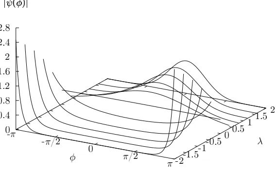
Figure 1. The wavefunction in angle representation for the intelligent states plotted for different values of λ. The transition from the truncated Gaussians in [8] to the large-uncertainty intelligent states forλ <0 is shown.
forλ >0 are the truncated Gaussians (3) [3, 8]. Formally this solution can be extended to negative values of λ [11]. For such negative values the wavefunction in the angle representation is given by
ψ(φ) = 1
N exp(− λ 2φ
2
) = 1 N exp(
|λ| 2 φ
2
), (17)
with the normalisation constant
N2 = Z π
−πexp(|λ|φ
2
)dφ=−i s
π
|λ|erf(i q
|λ|π). (18)
Note that the complex error function with a purely imaginary argument is also purely imaginary. Forλ <0 the wavefunction grows exponentially and is inversely proportional to the truncated Gaussians (see figure (1)). A state represented by this wavefunction can only exist because it is defined on a finite interval. For the case of linear momentum and position, where Gaussians are both the intelligent and constrained minimum uncertainty product states, solutions can also be characterised by a parameter λ. However, for the large-uncertainty case with λ < 0 the wavefunctions would not be normalisable and therefore not be elements of the Hilbert space.
3.1. Angle uncertainty
The square of the angle uncertainty is given by (∆φ)2 =
hφˆ2
i − hφˆi2. As our solutions
simply the expectation value of ˆφ2
(∆φ)2 = Z π
−πφ
2P(φ)dφ= 1
N2
Z π
−πφ
2exp(
|λ|φ2)dφ. (19)
The functional form of the wavefunction allows us to express the angle uncertainty as the derivative of the normalisation constant N with respect to|λ|:
(∆φ)2 = 1 N2
Z π
−π
d
d|λ|exp(|λ|φ
2)dφ= 1
N2
dN2
d|λ|. (20)
An expression for the angle uncertainty can be obtained on substituting the analytically exact normalisation constant (18) in (20):
∆φ = i s π
|λ|
exp(|λ|π2)
erf(iq|λ|π) − 1 2|λ|
1/2
. (21)
The largest angle uncertainty possible for intelligent states is ∆φ =π. This can be seen from (19) as P(π) is an even function of φ for the intelligent states:
(∆φ)2 = 2 Z π
0 φ 2
P(φ)dφ ≤2π2 Z π
0 P(φ)dφ=π 2
. (22)
The maximum value ∆φ = π is obtained in the limit of λ → −∞. A plot of ∆φ as a function of λ is shown in figure 2. For λ = 0 the flat angle probability density P(φ) = 1/(2π) gives the angle uncertainty of ∆φ = π/√3. The truncated Gaussians withλ >0 have a smaller angle uncertainty thanπ/√3 while the intelligent states with λ <0 considered here have a larger angle uncertainty.
3.2. Angular momentum uncertainty
Using the continuous wavefunction (17) and the representation of ˆLz as a derivative requires some care. In section 2 we have argued that for the intelligent states the first derivative of ψ(φ) with respect to φ represents a well behaved state, while the second derivative does not. This is the reason why we can use −i¯h(d/dφ) as a valid representation of ˆLz in the eigenvalue equation for the intelligent states. However, in the arbitrarily large state space of 2L+ 1 dimension reviewed in section 2 the angular momentum operator ˆLz is self-adjoint and Hermitian, and we may therefore write for the expectation value of ˆL2
z for the intelligent state |ψi:
hψ|Lˆ2
zψi=hLzψˆ |Lzˆ ψi=k |Lzψˆ i k2, (23) where k · k symbolises the norm of a state vector. The expectation value is a physical quantity and we can make now the transition to the continuous wavefunction ψ(φ) = hφ|ψi. Following the argument given above it is then valid to replace ˆLz with
−i¯h(d/dφ), allowing (∆m)2 to be written as
(∆m)2 = 1
¯ h2hLˆ
2
Large-uncertainty intelligent states for angular momentum and angle 8
Figure 2. The angle uncertainty ∆φfor the intelligent states. The parameter value λ= 0 distinguishes between the truncated Gaussians with λ > 0 [8] and the large-uncertainty intelligent states with λ <0. For intelligent states the angle uncertainty is bounded by ∆φ≤π.
On substituting the wavefunction (17) into this expression we find that the angular momentum uncertainty ∆m can be expressed in terms of the angle uncertainty ∆φ:
(∆m)2 = 1
N2
Z π
−π|λ|
2φ2exp(
|λ|φ2)dφ.=
|λ|2(∆φ)2. (25)
If we use the expression for the angle uncertainty ∆φfrom (21) we obtain for the angular momentum uncertainty ∆m:
∆m =|λ| i
s π
|λ|
exp(|λ|π2)
erf(iq|λ|π)− 1 2|λ|
1/2
. (26)
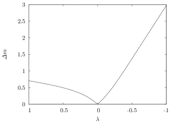
Figure 3. The angular momentum uncertainty ∆mplotted as a function ofλ. From (25), which also holds forλ > 0, one can see that ∆m tends to infinity for λ→ ∞. Forλ→ −∞, ∆mtends also to infinity and for this case the behaviour is visible in the plot.
3.3. Uncertainty product
The left hand side of the uncertainty relation (2) is given by the uncertainty product ∆m∆φ. Using the result for the angular momentum uncertainty ∆m (25) and the expression for ∆φ (21) the uncertainty product can be expressed as
∆m∆φ =|λ|(∆φ)2 = iqπ
|λ|exp(|λ|π
2)
erf(iq|λ|π) − 1
2 (27)
Large-uncertainty intelligent states for angular momentum and angle 10
Figure 4. Plot of the uncertainty product ∆m∆φ against ∆φ. For the large-uncertainty intelligent states (∆φ > π/√3 or λ < 0) the uncertainty product has no upper bound. The inset shows a plot of the uncertainty product against λ for comparison with the plots of ∆φand ∆m(see figures 2 and 3; see also a similar plot in [11])
3.4. Angular momentum distribution
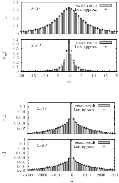
The probability amplitudes of the orbital angular momentum cm are calculated from the wavefunction (17) by means of a Fourier transform:
cm = √1
2π Z π
−πψ(φ) exp(−imφ)dφ. (28) By virtue of the symmetry of the wave function the transformation may be specialised to the Fourier cosine transform. The result can be expressed in terms of a complex error function
cm =
(−1)m N√2π exp
m2
2|λ| ! s
π 2|λ|2ℑ
erf
s
1
2|λ|m+ i s
|λ| 2 π
, (29)
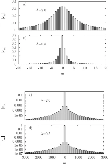
Figure 5. Orbital angular momentum distribution for different values of λ. a) λ=−2.0: A linear plot showing the distribution for the centralmvalues. b)λ=−0.5: linear plot. c)λ=−2.0: A logarithmic plot for the flanks. The width of the bars in the plot covers 100mvalues, but the shown value corresponds to them value in the middle of the bar. d)λ=−0.5: logarithmic plot.
4. Limiting behaviour
In the following we investigate the large-uncertainty intelligent states for two limiting cases to develop an understanding for the behaviour of the angle and angular momentum uncertainties. For small |λ| we present a perturbative approach, while for large λ we approximate the exponential in the wavefunction (17).
4.1. Small |λ| approximation
For small values of |λ|the continuous angle probability density becomes a flat function of the angle and in the limit of λ → 0, where P(φ) = 1/(2π) we have an angular momentum eigenstate. As we consider the case with zero angular momentum mean
Large-uncertainty intelligent states for angular momentum and angle 12
2L+ 1 dimension. For zero angle and angular momentum mean the condition for the intelligent state (15) can be written as
ˆ
Lz|ψi −iλφˆ|ψi= 0. (30) For small λ we can use the perturbation ansatz |ψi = |0i+λ|ϕ1i. Substituting this
ansatz in the condition (30) yields at first order in λ
λLzˆ |ϕ1i −i ˆφ|0i= 0. (31) Without loss of generality we can write the perturbative state |ϕi as a superposition of angular momentum eigenstates |mi, m = −L,−L + 1, . . . ,−1,1, . . . , L without a contribution from|0i:
|ϕ1i=
L X
m=−L/crcrm6=0
c1m|mi. (32)
The angular momentum eigenstate |0i is a physical state, that is a state which may be approximated to any desired accuracy by the expansionP
mbm|mi, where the coefficients bm = 0 for|m|> M. Here, the sum includes all integer values ofm and the boundM is sufficiently large to guarantee the desired accuracy but always less than L. Restricting the domain of the angle operator to these physical states simplifies the expression for the angle operator and changes the summation to include an infinite number of angular momentum states |mi. Using the definitions for the angular momentum operator and for the angle operator for physical states in [7] we can calculate the resulting states
ˆ
Lz|ϕ1iand ˆφ|0i:
ˆ Lz|ϕ1
i=
L X
m=−L/crcrm6=0
mc1
m|mi= L X
m=−L mc1
m|mi, (33)
ˆ
φ|0i = −i X m6=0
exp(imπ)
m |mi. (34)
On substituting these results in the condition for the intelligent states at first order in λ (31) we find an equation to determine the c1
m:
λ X m6=0
mc1
m−
exp(imπ) m
!
|mi= 0. (35)
For the linearly independent basis sates |mi the coefficients in (31) have to vanish to give zero as result. This requires c1
m =−(−1)m/m2. For small λ the perturbative state
|ψi may thus be written as
|ψi= 1 Nper
|0i −λ X
m6=0
(−1)m m2 |mi
, (36)
whereNperis the normalisation constant for the perturbative wavefunction. The angular
momentum amplitudes of the state|ψiare given byc0 = 1/Nperandcm =λc1m/Nper. The
allowLto tend to infinity, which yields the continuous wavefunction of the perturbative state:
hφ|ψi=ψ(φ) = 1 Nper
1
√
2π
1−λ X
m6=0
(−1)m
m2 exp(imφ)
= 1 Nper 1 √ 2π "
1 +λ π
2 6 − φ2 2 !# . (37)
The sum in the last equation has been evaluated using the contour integration method [15], which can also be used to calculate the normalisation from the requirement that the angular momentum probabilities |cm|2 sum to unity:
X
m |
cm|2 = 1 =
1 +λ2 X
m6=0
1 m4
= 1 +λ2 π4 45 ! 1 N2 per . (38)
The square of the uncertainty for the perturbative state can be calculated at first order from the continuous wavefunction (37):
(∆φ)2 =hφˆ2i= 1 N2 per
1 2π
Z π
−πφ
2
"
1 +λ π
2 6 − φ2 2 !# dφ. (39)
At first order in λ this leads to the angle uncertainty
∆φ ≈ √π
3
1− 2 15λπ
2, (40)
which explains the behaviour of ∆φ for small λ (see figure 6). The angular momentum uncertainty can be derived from the angle uncertainty according to (25). Because the angle uncertainty is multiplied by|λ|and the perturbative ∆φ from (40) is at first order λ this approximation holds for the second order inλ
∆m ≈ |λ|√π
3
1− 2 15λπ
2
. (41)
The behaviour of the angular momentum uncertainty in the perturbative approach is shown in figure 7. The equality in the uncertainty relation (2) at first order in λ can be seen directly from the results for ∆φ (40) and ∆m (41). The uncertainty product is given by
∆m∆φ =|λ|π
2
3 + O(|λ|
2) (42)
After substituting the expression forNperfrom (38) into the wavefunction (37), the right
hand side of the uncertainty relation becomes 1
2|1−2πP(π)| 1 2
1− 1−2|λ|π
2
3 + O(|λ|
2 ) !
=|λ|π
2
3 + O(|λ|
2
) (43)
Large-uncertainty intelligent states for angular momentum and angle 14
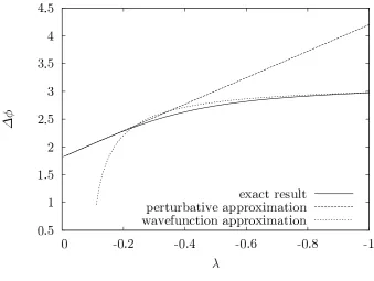
Figure 6.The angle uncertainty ∆φplotted for the analytically exact expression (21), in the perturbative approximation and in the wavefunction approximation (47). The wavefunction approximation fails for small values of|λ|. In this region a perturbative approximation can explain the behaviour of ∆φ.
4.2. Large |λ| approximation
In the approximation for large |λ| we approximate the wavefunction within an integration. This leads to two variants of this approximation: approximating the wavefunction in the normalisation integral gives a simple elementary expression, which can be used to calculate the angle and angular momentum uncertainties and hence the uncertainty product. We will refer to this approach as wavefunction approximation. On the other hand, applying this approximation under a Fourier integral to calculate the angular momentum probability amplitudes, allows us to explain the angular momentum distribution and to calculate the angular momentum uncertainty in this approximation. This approach will be called Lorentzian approximation as it explains the Lorentzian shape of the angular momentum distribution.
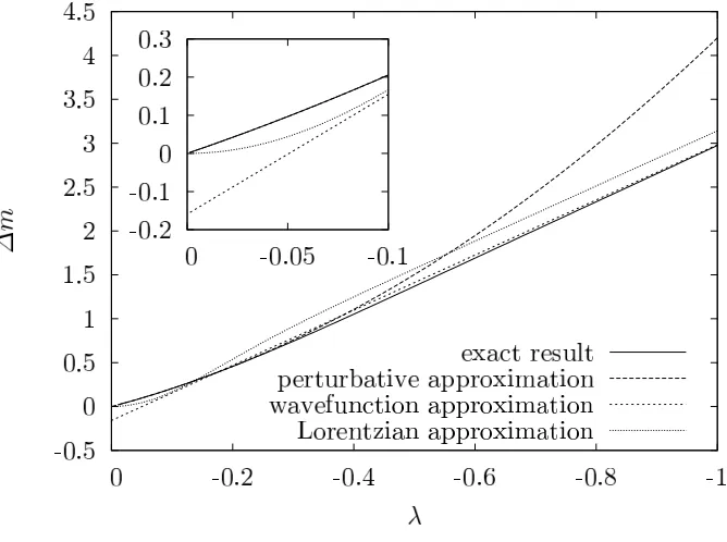
Figure 7. Plot of the angular momentum uncertainty for the exact result and different approximations. The expressions for ∆m in the wavefunction and perturbative approximation is derived from (25) by substituting the corresponding expression for ∆φ. For very small |λ| the perturbative approximation is indistinguishable from the exact result. The Lorentzian approximation originates from a summation of the Lorentzian angular momentum probabilities in (57).
The normalisation integral (18) can be rewritten as
N2 = 2 exp(
|λ|π2)Z 0
−πexp[|λ|(φ+π)(φ−π)]dφ. (44) For a large|λ|only a small region around−π will contribute significantly to the integral, and we can therefore approximate the factor (φ−π) in the exponential with −2π and extend the upper integration boundary to infinity. This results in the normalisation constant Nwvf
Nwvf2 = 2 exp(|λ|π 2
) Z ∞
−π exp(−2π|λ|(φ+π))dφ = 1
|λ|π exp(|λ|π
2
). (45)
Using this normalisation constant (45) in the expression for the probability density yields P(π) this approximation. From (17) we have:
P(π)≈ |λ|π for |λ|π2 >3. (46)
Large-uncertainty intelligent states for angular momentum and angle 16
hand side can be obtained using (20) and (25). Substituting Nwvf into (20) yields a
simple expression for the angle uncertainty:
∆φ ≈ |λ|π exp(|λ|π2)
d d|λ|
exp(|λ|π2)
|λ|π =π
2
− 1
|λ|. (47) A graph of the angle uncertainty is given in figure 6. One can see that the wavefunction approximation gives a good agreement with the analytical values for |λ| > 1/3 but fails for smaller values, where 1/|λ| grows without bound. The angular momentum uncertainty in this approximation follows from substituting ∆φ (47) in (25)
∆m ≈ |λ|π s
1− 1
|λ|π2 ≈ |λ|π−
1
2π. (48)
This approximate expression for ∆m gives a good approximation for large |λ|as can be seen in figure 7.
In the approximation for large values of|λ|the uncertainty product ∆m∆φis given as a simple function of |λ|. From (47) and (48) follows:
∆m∆φ ≈ |λ|π2−1. (49)
The right hand side of the uncertainty relation (2) contains the probability densityP(π) which is approximately |λ|π from (46) for |λ|π2
|>3. Therefore, 2πP(π) = 2|λ|π2 >1,
and the equality in the uncertainty relation is expressed by
|λ|π2
−1≃ |λ|π2
− 12 for |λ|π2 >3. (50)
Clearly, for sufficiently large values of |λ| the discrepancy becomes negligible. The approximation for large λ is based on our expression for Nwvf. If we refine the
approximation in (45) by setting exp[|λ|(φ+π)(φ−π)] = exp[−2π|λ|(φ+π)] exp[|λ|(φ− π)2] and expanding the second exponential according to exp[|λ|(φ−π)2]≈1+|λ|(φ−π)2,
we find that the expression for P(π) changes to
P(π) =λπ 1−1 2
1 π2|λ|
!−1
. (51)
Substituting this expression in the right hand side of the uncertainty relation (2) gives the equality with the uncertainty product (49). A plot of the uncertainty product is given in figure 8. Compared to the good agreement with the numerical values for the separate uncertainties ∆φ and ∆m, the discrepancies for the product appear to be large for the wavefunction approximation in figure 8. This is because ∆m=λ∆φ[cf. equation (25)] and as we have plotted the uncertainty product against ∆φ, the effect of an error in our approximation for ∆φ is enhanced in this plot.
4.3. Lorentzian approximation
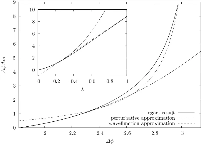
Figure 8. Plot of the uncertainty product ∆m∆φas a function of ∆φ. For negative λ ∆φ ranges between π/√3 and π. The curves are for the kernel wavefunction approximation for large|λ| and for the perturbative approximation for small|λ|. The inset shows the uncertainty product plotted as a function ofλ.
function. Owing to the symmetry of the wavefunction the Fourier cosine transform can be used:
cm = 2 N√2π
Z 0
−πexp(
|λ| 2 φ
2
) cos(mφ)dφ. (52)
In essence the integrand can be approximated in the same way as for the wavefunction approximation. The Fourier integrand can be written as exp[|λ|(φ + π)(φ − π)/2] exp(|λ|π2/2). Within the integration interval
−π ≤ φ < 0 and for large |λ| this Fourier kernel is only significantly different from zero around the lower boundary −π. This allows us to approximate the kernel with exp[|λ|(φ+π)(−π)] exp(|λ|π2/2) and to
extend the integration interval in (52) to infinity, which results in an angular momentum distribution in the shape of a Lorentzian:
cm ≈ 1
N√2πexp(
|λ| 2 π
2)Z ∞
−π exp(−π|λ|(φ+π)) cos(mφ)dφ,
= 1
N√2π(−1)
mexp(|λ| 2 π
2) 2|λ|π
|λ|2π2+m2
!
. (53)
Large-uncertainty intelligent states for angular momentum and angle 18
Figure 9. Orbital angular momentum distribution for different values of λ. a) λ=−2.0: linear plot shows the distribution for the central m values. b) λ=−0.5: linear plot. c) λ = −2.0: logarithmic plot for the flanks. The width of the bars in the plot covers 100mvalues, but the shown value corresponds to them value in the middle of the bar. d)λ=−0.5: logarithmic plot.
approximation for the two integrals in (53) and (45). One can see from figure (9) that the agreement with the Lorentzian is better at the flanks and for higher values of λ. This is consistent with our considerations as for larger values of |λ| the justification for the approximation of the wavefunction in the Fourier integral becomes more valid. Also, for central values of m the region around the upper boundary in the Fourier integral (52) contributes more. The angular momentum probabilities have to sum to unity. This condition can be used to calculate the normalisation constant within the Lorentzian approximation. We denote this approximate normalisation constant with NLor to distinguish it from the analytically exact value N. Using the results for the
probability amplitudes cm in (53) the sum of the probabilities may be written as:
∞
X
m=−∞
|cm|2 = 1 = 1 N2
Lor2π
4|λ|2π2exp(|λ|π2)
∞
X
m=−∞
The summation can be executed using contour integration [15], which results in the following expression for NLor:
N2
Lor = exp(|λ|π
2) πcosech2
(|λ|π2) + 1
|λ|πcoth(|λ|π
2)
!
. (55)
The angular momentum uncertainty can also be calculated from the angular momentum probabilities |cm|2 in the Lorentzian approximation (53) in the same way as
the normalisation constant NLor. From figure (9) and equation (53) it can be seen that
the angular momentum mean is zero. The square of the uncertainty is thus given by:
(∆m)2
≈ N21 Lor2π
4|λ|2π2exp(
|λ|π2)
∞
X
m=−∞
m2
(|λ|2π2+m2)2. (56)
Using again contour integration to evaluate the sum [15] and substituting the value of NLor we can write for the angular momentum uncertainty in the Lorentzian
approximation:
(∆m)2 = X m
|cm|2m2 (57)
≈π2
|λ|2coth(|λ|π 2)
− |λ|π2cosech2
(|λ|π2)
coth(|λ|π2) +|λ|π2cosech2(|λ|π2). (58)
For |λ|π2 > 3 this expression simplifies because the hyperbolic function cosech(|λ|π2)
becomes negligible small. In this limit we have
(∆m)≈π|λ|. (59)
The behaviour of the angular momentum uncertainty as a function of λ can be seen in figure (7).
5. Conclusion
We have studied the uncertainty relation for angular momentum and angle in a series of recent papers. The progress in creating and manipulating optical states with orbital angular momentum made it possible to confirm the form of the angular uncertainty relation experimentally for intelligent states, that is states which obey the equality in the uncertainty relation [8]. As the angular uncertainty relation has a state dependent lower bound, the intelligent states do not necessarily minimize the uncertainty product. We have explored the difference between the intelligent states and states, which give a minimum in the uncertainty product under additional constraints in a second paper [3]. In the present paper we emphasize the difference between intelligent states and minimum product states by introducing a class of intelligent states with arbitrarily large uncertainty product.
Large-uncertainty intelligent states for angular momentum and angle 20
product. We have derived analytical expressions for the angular momentum and angle uncertainties and the uncertainty product. In two limiting cases, for small negative λ and large negative λ we have explained the behaviour of the uncertainties with the parameter λ using approximate results. The three papers combined give an extensive overview of the uncertainty relation for angular momentum and angle.
Acknowledgments
We would like to thank David T Pegg for helpful discussions and we acknowledge financial support from the UK Engineering and Physical Sciences Research Council (EPSRC) under the grant GR S03898/01 and the Royal Society of Edinburgh.
References
[1] Heisenberg W 1927Z. Phys.43127
[2] Aragone C, Guerri G, Salam´o S and Tani J L 1974J. Phys. A: Math. Gen.7L149 Aragone C, Chalbaud E and Salam´o S 1976J. Math. Phys.171963
[3] Pegg D T, Barnett S M, Zambrini R, Franke-Arnold S and Padgett M 2005New J. Phys. 762 [4] Jackiw R 1968J. Math. Phys 9339
[5] Barnett S M and Pegg D T 1989J. Mod. Opt 367 Pegg D T and Barnett S M 1989Phys. Rev. A39 1665 Pegg D T and Barnett S M 1997J. Mod. Opt 44225
[6] Barnett S M and Radmore P 1997Methods in Theoretical Quantum Optics (Oxford: Clarendon Press)
[7] Barnett S M and Pegg D T 1990Phys. Rev. A41 3427
[8] Franke-Arnold S, Barnett S M, Yao E, Leach J, Courtial J and Padgett M 2004New J. Phys.6
103
[9] Allen L, Beijersbergen M W, Spreeuw R J C and Woerdman P 1992Phys. Rev A458185 Allen L, Barnett S M and Padgett M 2003 Optical Angular Momentum (Bristol: Institute of
Physics Publishing)
[10] Vaziri A, Weihs G and Zeilinger A 2002J. Opt. B: Quantum Semiclass. Opt.4S47
Leach J, Padgett M J, Barnett S M, Franke-Arnold S and Courtial J 2002, Phys. Rev. Lett. 88
257901
[11] Galindo A and Pascual P 1990Quantum Mechanics vol 1 (Berlin: Spinger Verlag) [12] Judge D and Lewis J T 1963Phys. Rev. Lett.5190
Carruthers P and Nieto M M 1968Rev. Mod. Phys.40 441 [13] Robertson H P 1929Phys. Rev 34163
Schr¨odinger E 1930Sitz. Preuss. Akad. Wiss.XIX 296
[14] Schwabl F 2002Quantum Mechanics 3rd edn (Berlin: Springer Verlag)

![Figure 4.Plot of the uncertainty product ∆comparison with the plots of ∆m∆φ against ∆φ.For the large-uncertainty intelligent states (∆φ > π/√3 or λ < 0) the uncertainty product hasno upper bound.The inset shows a plot of the uncertainty product against λ forφ and ∆m (see figures 2 and 3; see also a similar plotin [11])](https://thumb-us.123doks.com/thumbv2/123dok_us/1722269.125633/10.612.128.463.87.339/uncertainty-comparison-uncertainty-intelligent-uncertainty-uncertainty-gures-similar.webp)