arXiv:quant-ph/0512077 v2 27 Apr 2006
uncertainties
J¨org B. G¨otte†, Paul M. Radmore‡, Roberta Zambrini† and Stephen M. Barnett†
†Department of Physics, University of Strathclyde, Glasgow G4 0NG, UK
‡Department of Electronic & Electrical Engineering, University College London, London WC1E 7JE, UK
E-mail: [email protected]
Abstract. The uncertainty relation for angle and angular momentum has a lower bound which depends on the form of the state. Surprisingly, this lower bound can be very large. We derive the states which have the lowest possible uncertainty product for a given uncertainty in the angle or in the angular momentum. We show that, if the given angle uncertainty is close to its maximum value, the lowest possible uncertainty product tends to infinity.
Submitted to: J. Phys. B: At. Mol. Phys.
1. Introduction
If the lower bound in an uncertainty relation is state dependent, states satisfying the equality in the uncertainty relation need not give a minimum in the uncertainty product. This contrasts to the Heisenberg uncertainty principle for position and momentum [1], where the lower bound is a constant. Here, states which satisfy the equality in the uncertainty relation, that is intelligent states [2], also minimize the uncertainty product. The uncertainty relation for angular momentum and angle [3] however, has a state dependent lower bound requiring a distinction between intelligent states and minimum uncertainty product states [4]. These two kinds of states are defined as solutions of two different eigenvalue equations. For linear momentum and position the solutions to the two differential equations are the same Gaussians. In the angular case the two eigenvalue equations have two distinct solutions. Additionally, the angle is defined on a finite interval, allowing solutions to the differential equation which are disregarded in the linear case on the grounds that they do not represent physical, normalisable states on the infinite range on which position and linear momentum are defined. These solutions
are peaked at the edges of the 2πradian interval for the angle and consequently the angle
uncertainty of these states tends to be larger than for cases where the wavefunction is peaked in the middle of the interval and decays towards the boundaries. The intelligent and minimum uncertainty product states thus appear in two varieties with small and large angle uncertainties. The distinction is most apparent for the uncertainty product,
which is bounded from above by ~/2 for the states with small angle uncertainty, but
has no upper bound in the large-uncertainty case.
We should stress that in this work we will consider only the uncertainties in the angular momentum and in the associated angular coordinate [3]. This form of the uncertainty relation has been demonstrated to hold in a recent experiment [5] and underlies the security of a lately developed free-space communication system [6]. A range of other uncertainty relations have been derived in which measures of angular spread other than the angle uncertainty are used. These includes uncertainties based on trigonometric functions of the angle [7], discrete versions of the uncertainty relation [8] and entropic uncertainty relations [9].
The family of states related to the angular uncertainty relation has been investigated
in a series of previous articles. The form of the angular uncertainty relation has
from above and the uncertainty product reaches the global minimum for eigenstates
of the angular momentum operator ˆLz with uncertainty ∆Lz = 0. But one can also
consider states which minimize the uncertainty product under the constraint of a given uncertainty in either the angle or the angular momentum. It has been shown that states minimizing the uncertainty product are the same whether the additional constraint is a
given uncertainty in the angle ∆φor a given uncertainty in the angular momentum ∆Lz
[4]. These states are called constrained minimum uncertainty product (CMUP) states. In this article we will extend the analysis of CMUP states to the large-uncertainty
regime. An exact analytical solution for the wavefunction of these states will be
given in terms of complex confluent hypergeometric functions, but we also present an approximate solution in terms of Airy functions for the limiting case where the given
angle uncertainty ∆φ tends to its upper bound π. In particular we will compare this
kind of CMUP states with the large-uncertainty intelligent states.
2. Angular uncertainty relation
It is physically impossible to distinguish between two rotation angles differing by 2π
radians. Within the quantum mechanical description of rotation angles, this restricts
angle eigenvalues to lie within a 2π radian interval [θ0, θ0 + 2π) [3]. Choosing θ0
determines a particular 2π radian interval and with it a particular angle operator ˆφθ
and hence a basis set of angle eigenstates. In the following we adhere to the choice of
θ0 used in previous work [4, 5, 10] by setting θ0 = −π and dropping the label on the
angle operator ˆφ. The lower bound in the general form of the uncertainty relation for
two Hermitian operators is given by the expectation value of the commutator of these operators [11]. The commutator for angle and angular momentum operator is rigorously
derived in a finite state space Ψ of 2L+ 1 dimensions, spanned by the eigenstates |mi
of the angular momentum operator ˆLz with m ranging from −L,−L+ 1, . . . , L [3].
Only after physical results have been calculated in the finite dimensional space Ψ, L
is allowed to tend to infinity. It is in this limit of L → ∞ that the expectation value
of the commutator [ ˆLz,φˆ] can be approximated to an excellent degree for all physical
preparable states, which results in the angular uncertainty relation
∆Lz∆φ≥
1
2|1−2πP(π)|. (1)
Here, we are using units in which ~ = 1 and P(π) is the angle probability density at
the edge of the chosen 2π radian interval. This corresponds to our choice of θ0 = −π,
as the probability density is periodic in the angle and P(−π) = P(π). In general
different states used to calculate the uncertainties ∆Lz and ∆φ will have a different
angle probability densityP(π) rendering the lower bound in the uncertainty relation (1)
state dependent. From the uncertainty relation (1) it is evident why angular momentum eigenstates give a global minimum for the uncertainty product. For an eigenstate of the angular momentum operator the angle probability density takes on the constant value
equal to zero and so is the uncertainty product as the angular momentum uncertainty
vanishes and the angle uncertainty has the finite value of π/√3. This global minimum
in the uncertainty product is also the dividing point between small-uncertainty and large-uncertainty states. Away from this point the constrained minimum uncertainty
product (CMUP) states give a minimum in the uncertainty product for a given ∆φ or
a given ∆Lz.
3. CMUP states
Seeking states which minimize the uncertainty product for a given uncertainty in the angle or for a given uncertainty in the angular momentum is equivalent to minimizing the uncertainty that is not given. The corresponding equation for CMUP states has been derived in [4] using a variational method [12]. In this approach it is required that
a CMUP state|fiminimizes the uncertainty product, but with the constraint of keeping
the given variance constant and obeying the normalisation condition hf|fi = 1. The
additional constraints are taken into account by introducing undetermined Lagrange
multipliers [13]. In [4] it has been shown that for a CMUP state |fi the mean values
of angular momentum and angle can be set to zero, that is hLˆzi=hφˆi = 0. Therefore,
the variances (∆Lz)
2
and (∆φ)2
simplify tohLˆ2
ziand hφˆ 2
i respectively. The variation of
the uncertainty product with the given constraints thus results in a linear combination
of the variations δhLˆ2
zi, δhφˆ 2
i and δhf|fi, in which the Lagrange multipliers are the
coefficients:
δhLˆ2
zi+λδhφˆ 2
i=µδhf|fi. (2)
The linear combination is the same whetherhLˆ2
zi is given andhφˆ
2
iis minimized or hφˆ2
i
is given andhLˆ2
ziis minimized. Furthermore, it has also been demonstrated [4] that it is
admissible to consider only real coefficientsbm in the angular momentum decomposition
of |fiin the state space Ψ
|fi=
L X
m=−L
bm|mi. (3)
This allows us to write the variation δhf|Aˆ|fi for any Hermitian operator ˆA as
2(δhf|) ˆA|fi [13]. In particular this applies to the operators ˆL2
z,φˆ 2
and to the
identity operator ˆI corresponding to the variations δhLˆ2
zi, δhφˆ 2
i and δhf|fi. The linear
combination of variations in (2) thus turns into a linear combination of operators applied
to|fi. This leads to an eigenvalue equation of the form
ˆ
L2 z+λφˆ
2
|fi=µ|fi, (4)
where λ and µ are the Lagrange multipliers. The identification of the angular
momentum operator ˆLz as derivative with respect to φ sets additional requirements
on the wavefunction representing CMUP states [4, 10]. The wavefunction in the angle
representationψ(φ) =hφ|fihas to be an element ofC1
differentiable functions. The question of differentiability is of particular importance at
the boundaries of the 2π radian interval, on which the angle wavefunction is defined.
Whereas intelligent states are continuous, they do not have a continuous first derivative
at φ = ±π. CMUP states, however, do have a continuous first derivative at the
boundaries, and therefore representing ˆL2
z by the differential operator −(∂
2
/∂φ2
) is well defined. The eigenvalue equation (4) may thus be turned into a differential equation for
the CMUP wavefunction ψ(φ):
∂2
∂φ2ψ(φ) = λφ 2
−µ
ψ(φ). (5)
For the small-uncertainty case a solution of this equation has been given in terms of a confluent hypergeometric function in reference [4]. The angle wavefunction in this
regime is peaked at φ = 0 and λ, µ > 0 such that the curvature of the wavefunction
around φ = 0 is negative. For the large-uncertainty case the curvature around the
central region is positive and the multipliersλ, µ <0. Formally we can give the solution
to (5) in terms of confluent hypergeometric functions with complex arguments:
ψ(φ)∝exp −i|λ|
1 2
2 φ
2 !
M −i
4
|µ|
|λ|12
+1
4,
1
2,i|λ|
1 2φ2
!
, (6)
whereM is Kumer’s function [14]. This solution is obtained from (5) by settingλ=−|λ|
and µ=−|µ| for λ, µ <0 and using the same scaling as in [4], independent of the sign
of λ and µ: x = √2|λ|41φ and a = |µ|/(2|λ|
1
2). With these substitutions (5) takes on
the form
∂2
ψ ∂x2 +
x2
4 −a
ψ = 0, (7)
of which (6) is a solution with the appropriate change of variables. To evaluate the wavefunction and to calculate the angle and angular momentum uncertainty we have solved the scaled differential equation (7) numerically using a series expansion. In the
scaled form the wavefunction is characterized by the parameterawhich takes on positive
values for large-uncertainty CMUP states. The appropriate scaling is determined by the
condition that the positionx0 of the first maximum of ψ(x) corresponds toφ =π, such
that
φ= x
x0
π and |λ|= x
4 0
4π4. (8)
The value of x0 is determined numerically, so that the scaled wavefunction can be
normalised between −x0 and x0 allowing a calculation of the expectation value hxˆ
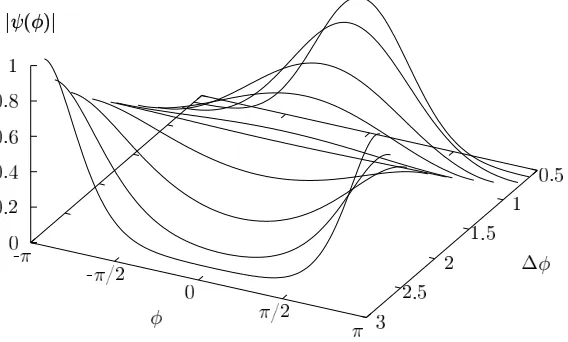
2
i by numerical integration. The transition of the wavefunction for the CMUP states from the small-uncertainty regime to the large-uncertainty regime is shown in figure 1. In connection with figure 1 it is useful to discuss qualitatively the consequences of the positive curvature in the central region of the wavefunction for the large-uncertainty CMUP states on the angle uncertainty. In [4] it has been shown that for CMUP states
with small ∆φthe single-peaked wavefunction has approximately the form of a Gaussian.
Figure 1. Plot of the wavefunction of CMUP states showing the transition from the small-uncertainty regime to the large-uncertainty regime. This distinction refers to the angle uncertainty ∆φ, and the dividing point is the flat wavefunction for ∆φ=π/√3.
deviates from the Gaussian form. For a = 0 the wavefunction is uniformly distributed
between−π and π and the angle uncertainty takes on the value of ∆φ=π/√3. This is
the dividing point between the small-uncertainty and large-uncertainty regime. If the
parametera is further increased then the curvature turns positive and the wavefunction
is peaked at ±π. Calculating the uncertainty or for such a CMUP state from the
variance ∆φ2
= hφˆ2
i − hφˆi2
yields values for ∆φ > π/√3. In the limit of a → ∞ the
angle uncertainty approaches the maximum valueπ [10]. In this limit, the 2π-periodic
angle probability distribution has a narrow peak centred at φ = π. The width of this
peak isnot ∆φ but rather the uncertainty in a different angle variable having a different
range of allowed angles (for example 0 to 2π). The angle uncertainty for a given state
depends on this choice of allowed angles in precisely the same way as does the phase uncertainty for a harmonic osscillator or a single electromagnetic field mode [15].
Using (8) the angle variance hφˆ2
i is given by hφˆ2
i = (π2
/x2 0)hxˆ
2
i for values of x in
[−x0, x0). The variance of the angular momentum operator is given by (5) in terms of
µ, λand hφˆ2
i, which results in the following expression for the product of the variances
hφˆ2
i and hLˆ2 zi:
hφˆ2
ihLˆ2 zi=hφˆ
2
iµ−λhφˆ2
i, (9)
=hxˆ2
i
−a+1
4hxˆ
2
i
. (10)
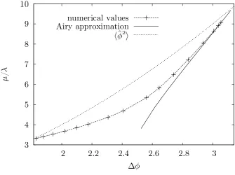
The limiting behaviour of the uncertainty product is directly connected to the behaviour
Figure 2. The ratio of the two Lagrange multipliersµandλdetermines the limiting behaviour of the uncertainty product (see equation (9)). For ∆φ → π the ratio µ/λ tends to π2, but more slowly than hφˆ2i. The uncertainty product thus tends to infinity. The plot ofµ/λin the Airy approximation shows the region of validity for this approximation.
µ/λ→π2
/3 (see figure 2). The variancehφˆ2
itakes on the value of π2
/3 and the overall
product of variances vanishes. For a → ∞, both µ and λ → −∞, but the ratio µ/λ
approaches π2
. The variance hφˆ2
i, however, tends to its maximum π2
faster than µ/λ
such that (9) tends to infinity. The resulting behaviour of the uncertainty product as
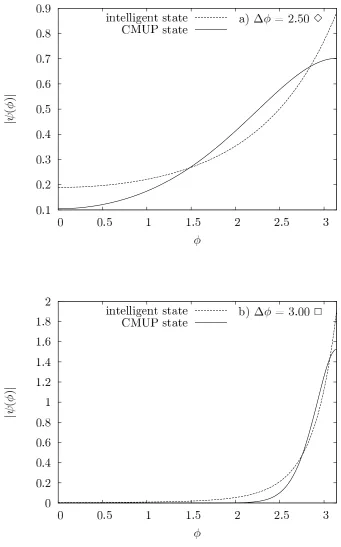
a function of ∆φ is given in figure 3. As in the small-uncertainty case for ∆φ < π/√3
the uncertainty product is smaller for the CMUP states than for the intelligent states while still obeying the uncertainty relation (1). This is possible because of the smaller
probability densityP(π) at the edge of the chosen 2πradian interval. Also, the difference
in the uncertainty product between intelligent states and CMUP states in the large-uncertainty regime is enhanced over the small-large-uncertainty regime. This goes along with a significant difference in the wavefunction for intelligent states and CMUP states for the
same ∆φ in this region (see figure 4). In the small-uncertainty regime the wavefunction
of intelligent and CMUP states both have approximately the same Gaussian form in
the region where the uncertainty product is 1/2 and changes only slowly with ∆φ. In
the large-uncertainty regime intelligent and CMUP states are of different form and we
will discuss an approximate expression for CMUP states in the limit of ∆φ → π later
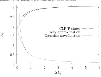
Figure 5. If the uncertainty product is minimized for a given uncertainty in the angular momentum, two minima can be obtained. The first and smaller minimum is obtained for the small-uncertainty CMUP states while a secondary minimum is found for the large-uncertainty CMUP states. For comparison the limiting cases for these two kinds of states are shown. For ∆φ→0 the small uncertainty states become Gaussians [4], whereas the large-uncertainty states are approximatively given by Airy functions for ∆φ→π.
In connection with figure 3 it is appropriate to clarify the meaning of minimizing the uncertainty product under a constraint. For CMUP states with small and large angle uncertainties the angular momentum uncertainty can take on all positive real
values. ∆Lz is zero for the angular momentum eigenstates at ∆φ = π/
√
3 and it
approaches infinity for ∆φ → 0 and ∆φ → π. Minimizing the uncertainty product
for a given ∆Lz yields two constrained minima. The smaller constrained minimum is
obtained for the small-uncertainty CMUP states and corresponds to an angle uncertainty
∆φ < π/√3. A secondary minimum, however, is obtained for the large-uncertainty
CMUP states corresponding to ∆φ > π/√3 (see figure 5). On the other hand minimizing
the uncertainty product for a given ∆φ results in a unique minimum. Whether this
minimum is obtained for small-uncertainty or large-uncertainty CMUP states depends
on the given ∆φ.
the wavefunction in terms of Airy functions, which allows us to calculate the variance
∆φ analytically.
4. Airy approximation
The defining differential equation for the CMUP states (5) can be approximated and the resulting equation solved to give an analytical expression for the CMUP wavefunction
in the limiting case ∆φ→π, as we now describe.
The behaviour of the solution for a general differential equation of the form
∂2
ψ
∂x2 =P(x)ψ(x) (11)
is partly determined by the sign of the functionP(x). ShouldP(x) be purely positive we
would expect an exponential behaviour, whereas for a purely negativeP(x) the solution
would be oscillating. Of particular importance, therefore, are the values of x where
P(x) exhibits a change of sign, that is the turning points of the equation (11). We
can restrict the analysis of the differential equation (5) to the half interval [0, π) due
to the symmetry of the equation. In this range equation (5) has one turning point at
φ =pµ/λ. The equation is approximated by expanding P(x) = λφ2
−µ around this
turning point. Settingφ=p
µ/λ+xand neglecting quadratic terms inxturns (5) into
Airy’s equation [17]
∂2
ψ
∂y2 =yψ, y=−(2
p
µλ)13x=−(2pµλ) 1
3(φ−pµ/λ). (12)
This equation is solved exactly by the Airy function Ai(y) which results in
ψ(φ) =CAi−(2pµλ)13(φ− p
µ/λ) (13)
on substituting the appropriate variables. Here, C is the normalisation constant. To
fulfill the boundary condition ψ′
(π) = 0 the argument of the Airy function in (13) is
required to have the value of the first zero of Ai′
for φ=π. This leads to the equation
−(2pµλ)13(π−pµ/λ) = −1.0188. (14)
Choosing a particularλgives a quartic equation forpµ/λand for values ofpµ/λclose
toπ an approximate solution is given by
µ
λ ≈π−
−1.0188
2λπ
13
. (15)
In the Airy approximation a particular CMUP state can thus be characterized by the
Lagrange multiplier λ. The normalisation constant can be determined by analytical
evaluation of the normalisation integral
1 = 2
Z π
0
ψ2
(φ)dφ≈2C2
2pµλ
−1
3 Z
∞
−1.0188
Ai2
(y)dy. (16)
In the last step we have extended the range of integration from y(φ = 0) =
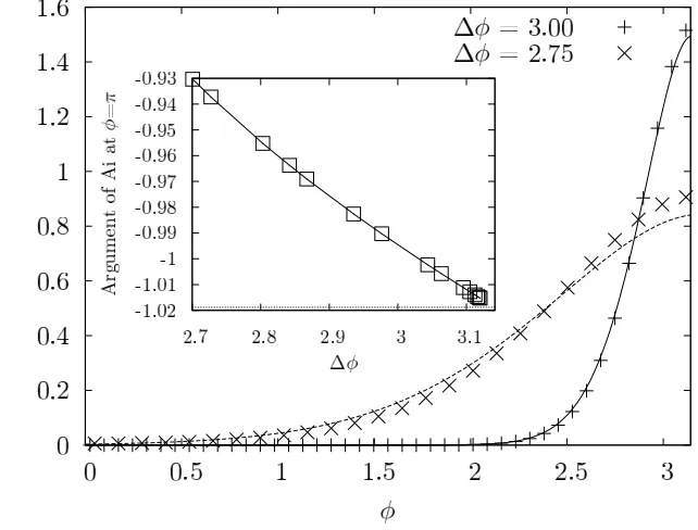
Figure 6. Plot showing a comparison of the Airy approximation (continuous lines) with the numerical calculated wavefunction (individual points). For ∆φ= 3 (+) the Airy approximation shows a good agreement with the numerical results. The inset shows the deviation of the argument of the Airy function Ai atφ=π from −1.0188 (marked by the horizontal dotted line), the position of the first maximum of the Airy function Ai.
(∆φ → π), the wavefunction decays to zero sufficiently quickly for small angles so
that extending the upper bound in the integral does not significantly change the normalisation integral. Primitives of products of Airy functions can be calculated using the method of Albright [18]. This results in
C= (µλ)121
(1.0188)12(0.5357)2
1 3
−1
, (17)
where Ai(y = −1.0188) = 0.5357. In figure 6 a comparison of the numerically
calculated wavefunction and the wavefunction in the Airy approximation is shown. The
approximation becomes better for values of ∆φ closer to π. An inset in figure 6 gives
the deviation of the argument of the Airy function in (13) from the exact value of
y = −1.0188 due to the approximation (15) of the quartic equation (14) determining
µ/λ.
Within the Airy approximation the integral for the angle variance can be calculated analytically using the method of Albright [18]:
(∆φ)2
= µ
λ +
2
3(1.0188)
2pµλ
−1
3 p
Figure 7. Comparison of the uncertainty product calculated in the Airy approximation and for numerical results. In difference to figure 3, the graph shows only the large-uncertainty region (∆φ > π/√3) and the ordinate is extended to larger values of ∆φ∆Lz. The Airy approximation explains the behaviour of ∆φ∆Lz in a
region where our numerical calculation fails.
+ 1
5(1.0188
−1
+ 1.01882
)2pµλ
−2
3
. (18)
As in the calculation of the normalisation constant (16) the upper boundary in the
integration has been extended to infinity. On multiplying (18) by λ one can see in
(9) that λhφˆ2
i will always be smaller than µ resulting in an unbounded uncertainty
product. Within the Airy approximation the uncertainty product can be calculated for
values of ∆φ much closer to π than in the numerical calculation. This is due to the
fact that our numerical determination of the first maximum fails for large values of a.
In the Airy approximation a numerical search for the first maximum is not necessary. The uncertainty product calculated in the Airy approximation is compared with the numerical results in figure 7.
5. Conclusion
satisfying the equality in the uncertainty relation, to be distinct from constrained minimum uncertainty product (CMUP) states. These states minimize the uncertainty product for a given variance in angle or for a given variance in angular momentum. Also, in contrast to the linear position, the angle is defined on a bounded interval. Therefore, wavefunctions peaked at the edge of the interval are normalisable and can represent physical states. Intelligent and CMUP states are defined by two different eigenvalue equations. For the angular uncertainty relation the solutions to the eigenvalue equations are angle wavefunctions which are peaked in the middle or peaked at the edge. This gives rise to two varieties of states with small and large angle uncertainties respectively. Intelligent states with large angle uncertainties may have arbitrarily large uncertainty products while still satisfying the equality in the uncertainty relation. Similarly, CMUP states with large-angle uncertainties minimize the uncertainty product locally or globally for a given constraint. The obtained minimum uncertainty product may be very large. It depends on the given uncertainty whether the minimum is local and the small uncertainty CMUP states give a smaller uncertainty product, or if the large-uncertainty CMUP state gives the smallest possible constrained uncertainty product.
Intelligent states with small and large angle uncertainties have been discussed previously in two papers [5, 10], while the CMUP states with small angle uncertainties
have been studied in a third paper [4]. Here, we have examined CMUP states
with large angle uncertainties. We have found an analytically exact solution for
the CMUP eigenvalue equation in terms of confluent hypergeometric functions with complex arguments. We also have solved the equation numerically and have calculated
the angle uncertainty from this solution by numerical integration. To explain the
limiting behaviour for sharply peaked wavefunctions we have developed an analytical approximation using an expansion about a turning point. The approximate solution is given as the decaying tail of the Airy function Ai. Within this approximation we were able to calculate the uncertainty product analytically.
We have found that the difference in the uncertainty product between intelligent
states and CMUP state is enhanced in the large-uncertainty regime. In [4] the
possibility to distinguish between intelligent states and CMUP states in an experiment was discussed. While it might be more difficult to prepare large-uncertainty states in an experiment, the greater difference in the uncertainty product could simplify the experimental evaluation significantly. The difference between CMUP and intelligent states in the large-uncertainty regime is also a clear indication for the necessary distinction between the two regimes and shows that large-uncertainty states cannot
be transformed into small-uncertainty states by shifting the the 2π radian range, but
should be treated separately.
Acknowledgments
(EPSRC) under the grant GR S03898/01.
References
[1] Heisenberg W 1927Z. Phys.43127
[2] Aragone C, Guerri G, Salam´o S and Tani J L 1974J. Phys. A: Math. Gen.7L149 Aragone C, Chalbaud E and Salam´o S 1976J. Math. Phys.171963
[3] Barnett S M and Pegg D T 1990Phys. Rev. A41 3427
[4] Pegg D T, Barnett S M, Zambrini R, Franke-Arnold S and Padgett M 2005New J. Phys. 762 [5] Franke-Arnold S, Barnett S M, Yao E, Leach J, Courtial J and Padgett M 2004New J. Phys.6
103
[6] Gibson G, Courtial J, Padgett M, Vasnetsov M, Pas’ko M, Barnett S M and Franke-Arnold S 2004
Opt. Express 125448
[7] Holevo A 1982Probabilistic and statistical aspects of quantum theory(Amsterdam: North Holland) Yamada K 1982Phys. Rev. D 253256
Goh S S and Goodman T 2003Appl. Comput. Harmon. Anal.1619 [8] Brody D C and Meister B K 1999J. Phys. A: Math. Gen.324921 [9] Deutsch D 1983Phys. Rev. Lett 50631
S´anchez-Ruiz J 1993Phys. Lett. A 181193
[10] G¨otte J B, Zambrini R, Franke-Arnold S and Barnett S M 2005J. Opt. B: Quantum Semiclass. Opt.7S563
[11] Robertson H P 1929Phys. Rev 34163
Schr¨odinger E 1930Sitz. Preuss. Akad. Wiss.XIX 296 [12] Jackiw R 1968J. Math. Phys 9339
[13] Summy G S and Pegg D T 1990Optics Communications 7775
[14] Abramowitz M and Stegun I A 1974 Handbook of Mathematical Functions (Mineola: Dover Publications)
[15] Barnett S M and Pegg D T 1989J. Mod. Opt 367 Barnett S M and Pegg D T 1997J. Mod. Opt 44225
[16] Galindo A and Pascual P 1990Quantum Mechanics vol 1 (Berlin: Spinger Verlag) [17] Jeffreys H 1942Phil. Mag 33 451
Radmore P 1980J. Phys. A: Math. Gen.13173 [18] Albright J R 1977J. Phys. A: Math. Gen.19485