Factorization techniques in robust controller design

(V

F a c to r iz a tio n T e c h n iq u e s

in

R o b u s t C o n tr o lle r D e s ig n

A n d r e w J a m es T elford

B .E . H on s. (J C U N Q )

October 1989

A thesis subm itted for the degree of Doctor of Philosophy

of the Australian National University

D e c la r a tio n

These doctoral studies were conducted under the supervision of Professor John B. Moore, and much of the work has been recorded elsewhere in con­ ference proceedings or journals (see [35, 34, 44, 45, 43, 36]).

The content of this thesis, except as otherwise explicitly stated, is the result of original research, and has not been submitted for a degree at any other university or institution.

Andrew Telford,

A c k n o w le d g e m e n ts

First of all I wish to thank my supervisor John Moore for allowing me the opportunity to work with him over the past few years, for guidance in aca­ demic and personal matters, for sharing his enthusiasm about research, and for making himself available at all times.

Thanks are also due to others in the Department of Systems Engineering for help with academic problems, as well as for their friendship and hospital­ ity. In this respect I would particularly like to mention Bob Bitmead, Brian Anderson, Phillip Musumeci, and Xia Lige. I consider it great fortune to have been part of such a dynamic research environment.

Coming to Canberra has involved many changes, including moving away from my family, but neverless it has been an exciting time. I have been blessed to have made so many friends here. Thanks to Christine, Meredith, and Natalie for sharing a house with me, and to the families at Reid church who have opened their homes to me. A special thanks to my fiancee Heather, who has given me so much love, support, and prayers over this last year.

I dedicate this thesis to my mother and father, whose love and personal sacrifice over the years has enabled me to have so much,

Andrew Telford

A b str a c t

This thesis is concerned with the design of robust controller algorithms. The mechanics of the design procedures involve factoring the plant and controller transfer functions into stable, proper factors. This has the advantage of allowing the analysis of the stability properties of the control loop, and, for instance, enabling the characterization of the class of all stabilizing controllers for a given plant.

Here results are developed showing that the class of all stabilizing con­ trollers for a given plant can be structured as a state estimate feedback controller, with the state feedback and state estimate gains generalized to be proper transfer functions. This result is also generalized to the case of reduced-order observers. An important by product of the work on reduced order observers is the generation of new state-space realizations of doubly co- prime factorizations; these state-space realizations are important both from a theoretical point and a computational point of view.

An arbitrary controller can be organized as a state estimate feedback controller with a constant state feedback and state estimator gain provided that the solution to a particular quadratic matrix equation exists. The in­ sights gained by studying this realization problem lead to an investigation of conditions under which the solutions of of the algebraic Riccati equation exist.

Some related work on the problem of controller reduction follows. A

troller reduction scheme is proposed which applies standard model reduction algorithms to augmentations of the controller which arise when working with the class of all stabilizing controllers. Practical issues such as scaling of the plant variables are addressed, and two examples are given to demonstrate the use of the model reduction techniques.

P r e f a c e

The m aterial in this thesis is th e result of joint research w ith my supervisor Professor John Moore. T he contributions I particularly identify w ith are

summarized as follows:

• My introduction to research was an involvement w ith a project initiated by Prof. Jo h n Moore and Prof. K eith Glover. This work on factor­ ization theory and frequency-shaped state estim ate feedback control appears in C h ap ter 2. I was responsible for taking th e initial ideas, finding and correcting m ajor errors in th e theorem s, and producing the results in th eir final form.

• T he ideas in C hap. 3, on solution of the nonsym m etric Riccati equation, and Chap. 6, on adaptive resonance suppression, resulted from joint work w ith Prof. John Moore and myself. I provided m any of the theoretical ideas and all of th e sim ulation results.

• The work on controller reduction in Chap. 5 was also done w ith the Prof. John Moore— In p articu lar, I was responsible for formalizing m any of th e theoretical aspects of the chapter. Prof. Uy-loi Ly provided realistic aircraft models to test th e controller reduction algorithm s.

• After initial discussions w ith Prof. Moore, I carried out alm ost all of th e research in C hap. 4 independently. This work is concerned with doubly coprime factorizations related to reduced order observers.

C o n t e n t s

L ist o f F ig u r e s x i

L ist o f T a b le s x iv

N o t a t io n x v

1 I n tr o d u c tio n 1

2 A ll s ta b iliz in g c o n tr o lle r s as fr e q u e n c y s h a p e d s t a t e e s t im a te

fe e d b a c k 11

2.1 In tro d u ctio n ... 11

2.2 Stabilizing controllers for G, Gf, Gh ... 17

2.3 Stabilizing controllers for G in terms of Qp, Qh, Q ... 26

2.4 Useful relatio n sh ip s... 32

2.5 C o n c lu sio n s... 33

A2.1 Some basic definitions ... 34

A2.2 P r o o f s ... 36

3 O n t h e e x is t e n c e o f s o lu tio n s o f n o n s y m m e tr ic R ic c a t i e q u a ­

tio n s 42

3.1 In tro d u c tio n ... 42

3.2 The scalar c a s e ... 44

3.3 The multivariable c a s e ... 49

3.4 C o n c lu sio n s... 53

A3.1 Alternative proof of Theorem 3 . 5 ... 54

4 D o u b ly c o p r im e fa c to r iz a tio n s , r e d u c e d o rd er o b s e r v e r s, a n d d y n a m ic s t a t e e s t im a t e fe e d b a c k 56 4.1 In tro d u c tio n ... 56

4.2 Factorizations related to minimal-order o b s e r v e r s ... 57

4.2.1 Preliminaries ... 57

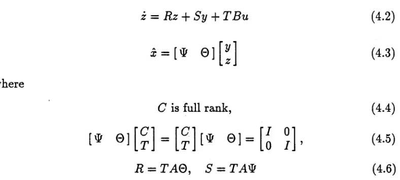
4.2.2 F acto rizatio n s...59

4.2.3 The class of all stabilizing c o n tro lle rs... 62

4.3 Dynamic state estimate f e e d b a c k ...65

4.3.1 F acto rizatio n s...66

4.3.2 All stabilizing controllers as minimal-order observer-based c o n tr o lle r s ... 72

4.4 The minimal-order dual observer ... 75

4.5 C o n c lu sio n s... 77

5 C o n tr o lle r r e d u c tio n m e t h o d s m a in ta in in g p e r fo r m a n c e a n d

r o b u s tn e s s 79

5.1 In tro d u c tio n ... 79

5.2 Details of controller reduction ... 84

5.2.1 D efinitions...84

5.2.2 S calin g ... 86

5.2.3 Re-Optimization ... 89

5.2.4 Estimation-based reduction ... 90

5.2.5 Controller reduction maintaining p e rfo rm a n c e ...92

5.2.6 Frequency shaped r e d u c tio n ... 92

5.2.7 Generation of F, H ... 94

5.2.8 Staged r e d u c tio n ... 95

5.2.9 Simultaneous s ta b iliz a tio n ... 95

5.2.10 Reduced order p l a n t ...97

5.3 Rationale ... 97

5.3.1 Preserving robustness p ro p erties... 97

5.3.2 Closeness m e a s u re s ... 99

5.4 Examples ...101

5.5 C o n c lu sio n s...105

6 A s t u d y on a d a p tiv e s ta b iliz a t io n a n d r e s o n a n c e s u p p r e s sio n 106 6.1 In tro d u ctio n ...106

6.2 An adaptive algorithm for resonance suppression... 109

6.3 A Simulation S tu d y ...114

6.3.1 Preliminary Results with Standard Pole Assignment . . 114

6.3.2 Closed-loop Poles Adaptively A s sig n e d ... 116

6.3.3 Cautious C o n tr o l... 118

6.3.4 Central Tendency Adaptive Pole A ssignm ent... 119

6.3.5 Transient Performance Simulation R e s u l t s ... 121

6.4 Preconditioning M e th o d s... 122

6.5 C o n c lu sio n s... 129

7 C o n c lu s io n s a n d F u r th e r R e se a r c h 130 7.1 C o n clu sio n s... 130

7.2 Further research ... 134

L is t o f F ig u r e s

2.1 Closed loop s y s te m ... 12

2.2 Control system with state fe e d b a c k ... 12

2.3 An asymptotic state e s tim a to r... 14

2.4 Class of all stabilizing c o n tr o lle r s ... 22

2.5 Class of all stabilizing controllers: Doyle-Stein f o r m ...23

2.6 Stabilizing controllers F( Qf), H( Qf) ... 26

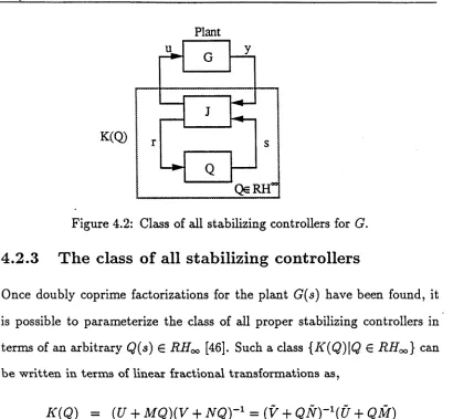
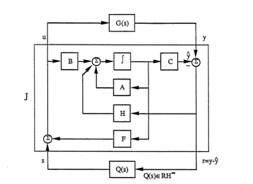
2.7 Class of all stabilizing state estimate feedback controllers, de­ noted K[ F( Qf ), H( Qf) , Q ]... ’...30

3.1 Plant/controller feedback p a i r ...43

4.1 Minimal-order observer based control l o o p ... 59

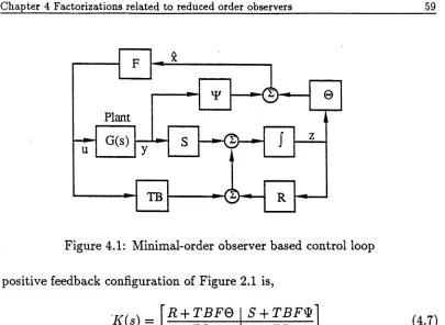
4.2 Class of all stabilizing controllers for G... 62

4.3 Controller class {K(Q)\Q E RHoo} based on full-order observer 64 4.4 Controller class {K(Q)\Q E RHoo} based on minimal-order o b s e r v e r ... 65

4.5 Feedback loop containing Gf and F ... 71

4.6 Observer based controller with dynamic state estimate feedback. 72 4.7 Reduced order observer-based control l o o p ... 78

5.1 Feedback structures based on the class of all stabilizing con­ trollers ... 82 5.2 Controller c l a s s ...85 5.3 Estimation-based reduction ... 91 5.4 New J and Q blocks based on controller designed for simulta­

neous stabilization of many plants... 96 5.5 Linear fractional m a p s ... 99 5.6 Block diagram of the flutter suppression and gust load allevi­

ation sy s te m ... 102 5.7 Frequency-weighting at the controller i n p u t s ...104

6.1 Main control s y s t e m ... 110 6.2 Pole assignment with the dominant resonant mode assigned

radially in w a rd s... 113 6.3 Frequency response of second-order lightly damped transfer

f u n c t i o n ...115 6.4 Estimate of the frequency lj\ of the least stable pole pair . . . 123

6.5 Estimate Qo,k generated by outer identifier(RLSo ) ... 124 6.6 Plant o u tp u t... 125 6.7 Plant/noise m odel...126

6.8 Adaptive scheme to enhance fixed controller d e s i g n ...128

7.1 Alternative stability re g io n ...131

L ist o f T a b le s

5.1 Reduction of a 55th order Flutter Suppression and Gust Load Alleviation Controller...103

6.1 Simulation results: Adaptive pole positioning... 117

N o t a t i o n

W here fu rth e r ex p lan atio n of th e sym bol is needed, a page n u m b er is given.

c field of com plex num bers

C n ,m n x m m atrices over th e field of com plex num bers Hoo a H ardy space, p.34

JnW

£[•] Laplace tran sfo rm

A(A) set of eigenvalues of th e m a trix A

Loo

R field of real num bers

K n , m n x m m atrices over th e field of real num bers RHoo real-ratio n al H ardy space, p.34

R P p ro p er tran sfer functions, p.34

R Sp stric tly proper tran sfer functions, p.34

x ( t ) tim e derivative of x ( t )

4 estim ate of th e q u a n tity q

II lU Hoo norm , p.34

X - R

a r i g h t in v e r s e o f X

X - L _{a le ft in v e r s e o f X}

X ' t r a n s p o s e o f X

X * H e r m i t i a n c o n j u g a t e o f X A B

s t a t e s p a c e r e a l iz a t i o n , p .3 5

rP

c D

C h a p ter 1

In tr o d u c tio n

Classical controller design and analysis techniques are based on frequency domain concepts and are principally concerned with the control of single­ input single-output plants. Such techniques are adequate for a large class of practical engineering design problems: they are simple to understand, do not need complex hardware, and are reliable. In addition, gain/phase margins, Nyquist diagrams, and Bode plots are examples of concepts and tools which can be used to analyse the feedback loop.

There are, however, control problems which cannot be treated using sin­ gle loop control techniques: a plant may be controlled from more than one input and measurements may be taken from many outputs. Classical con­ trol techniques are generally inadequate for use with multivariable plants, although knowledge of classical theory provides a good background for the study of multivariable systems.

The introduction of the idea of the state of a linear system into the

Chapter 1 Introduction 2

trol literature was a major step forward in the treatm ent of multivariable systems. State space ideas arise naturally in the mathematical treatm ent of linear ordinary differential equations, and engineers often model systems using such differential equations. Consider as an example the following state space system G : u(t) i-+ y(t),

x(t) = A(t)x(£) + B(t)u(t);

y(t) = C(t)x(t) + D(t)u(t) (1.1)

where for any time t, A(t) E IRn,n, B(t) E lRn,m, and C(t) E lRp,n- The system (1.1) along with initial conditions for x(t) defines the relationship between the m x 1 input vector u(t) and the p x 1 output vector y(t). The n x l state vector x(t) is defined by a vector differential equation driven by u(t); the output vector y(t) is a linear combination of x(t) and u(t). Much of what follows is concerned with the class of time-invariant state space systems, where A(t), B(t), and C(t) are restricted to be constant real matrices. In this case Laplace transform techniques provide an alternative representation of G. Assuming zero initial conditions,

Y( s ) = G(s)U(s) (1.2)

G(s) = C ( s l - A)~XB + D (1.3)

where L'(s) = £[y(t)]-, U(s) = C[u(t)}

Chapter 1 Introduction 3

represent physical variables, either measurable or unmeasurable. In some situations it is desirable to obtain on-line estimates of the state variables, ei­ ther for monitoring unmeasurable physical variables, or for use in the control algorithm. Much of linear control theory is concerned with regulation of the state x(t) to some reference state by appropriate manipulation of the control input. The problem of on-line estimation of the state via observers (state estimators) has been an important research topic over the last thirty years, with im portant initial contributions by Kalman [19] and Luenberger [27].

Chapter 1 Introduction 4

design and Kalman filtering problems are strict mathematical duals, with a controller formed by the cascade of a Kalman filter and an LQ controller known as a linear quadratic gaussian (LQG) controller.

Although LQG control seems like an ideal optimal control strategy, there are some im portant problems that arise in practice. One such problem is ro­ bustness to uncertainty in the plant model: the closed loop system may not be stable if the true plant is slightly different from the nominal plant. This is in contrast to the scalar LQ controller, where it can be shown that there is an inherent infinite gain margin and a corresponding 60° phase margin [3]. The problem of robustness to plant uncertainty or small time variations in the plant model is one that becomes more important as control systems be­ come more complex, since plant error can be roughly compared to controller realization error. In the LQG case, techniques such as loop transfer recovery [13] have been proposed to obtain a compromise between the optimality and robustness.

State space realizations such as (1.1) or (1.3) are not the only ways to represent the input-output behaviour of dynamical systems. In Wolovich [48] and [18] there is a treatm ent of linear time invariant systems represented by ratios of polynomial matrices. Canonical forms and properties such as minimality can be described for polynomial factor representations as has been done for state space systems.

Chapter 1 Introduction 5

of a multivariable system. The transfer function is factored into matrices of

stable, proper transfer functions. Although stable, proper factorizations may seem to be unnecessarily complex, they have the advantage of being useful when analysing the stability of a feedback system. For instance, using stable proper factorizations it is possible to characterize the class of all stabilizing controllers for a given plant, a concept which is very important in this thesis. This factorization approach to controller synthesis and analysis was intro­ duced by Kucera [22] for discrete time and Youla et. al. [49] for continuous time, and later formulated in an axiomatic framework [11, 46]. It provides a framework for research in the area of Hqq optimal control [15], which is con­ cerned with finding a controller to minimize the norm of a disturbance transfer function subject to the constraint that the controller be stabilizing.

Many of these results at first sight seem irrelevant to practical control en­ gineering, because of the abstract algebraic framework which underlies much of the theory. This thesis is concerned principally with using ideas, tech­ niques, and results from the factorization approach in the design of practical robust controllers. Existing knowledge and intuition based on frequency do­ main ideas is combined with the new theory. A summary of the progression of ideas in the thesis now follows.

S tate estim ate feedback Chapter 2 is concerned with the design of

C h ap ter 1 In troduction 6

the class of all stabilizing controllers for a given plant can be obtained using a state estimate feedback control structure. The control signal is formed by adding a linear function of the state estimate to a stable filtering Q(s)r of the residuals r, where the residuals is the difference between the true plant output

y and estimate y of the plant output from the state estimator. The class of all stabilizing controllers for a given plant is obtained by varying the parameter Q(s) over the class of all stable transfer functions. In Doyle’s work the state feedback gain and the state estimator gain are constant real matrices, whereas this thesis allows them to be possibly unstable transfer function matrices. We will sometimes refer to the dynamics in the state estimator and state feedback gains as frequency shaping, because the frequency response of the dynamics can sometimes be related to plant or plant noise frequency responses.

Chapter 1 Introduction 7

A lgebraic R iccati equations Following on from this, one can ask

when an arbitrary controller can be organized as a state estimate feedback controller with a constant state feedback law and a constant state estimator gain. It was originally observed by Anderson [1] that this is possible only when there exists a nonsingular solution to a particular nonsymmetric Riccati

equation. Such equations also arise in polynomial factorization theory [9], and although they have been treated at length in the literature, some of their properties are less well understood than for the symmetric case.

Chapter 3 provides contributions to established theory on this funda­ mental subject. Necessary conditions are shown for solutions of this Ric­ cati equation to exist in terms of controllability and observability of the plant/controller state space realizations. The existence of an inverse of these solutions is given by considering a dual Riccati equation. There is also an alternative proof to that given hitherto, to establish the sufficiency of these conditions for a class of equations associated with certain scalar variable problems. A counterexample is given to the conjecture that the sufficiency conditions can be extended, without modification, to the multivariable case. This leads to generalized conditions for the multivariable case. As a challenge to the reader, it is conjectured that these are also sufficient conditions.

R educed order observers; doubly coprim e factorizations To make

Chapter 1 Introduction 8

transfer functions. For convenient computation, is it desirable to be able to work with state-space realizations of these transfer functions. In important work by Nett, Jacobson, and Balas [39], explicit state-space realizations of these factorizations are derived using results from state estimation and state feedback theory. These results are based only on full-order state estimators, which have realizations with the same McMillan degree n as the plant model.

Asymptotic state estimation can also be achieved by estimators of a lower degree: the degree may be reduced to n — p for a plant with p outputs. This theory on reduced-order observers was originally reported by Luenberger [27], and is a generalization of the full-order case. In Chap. 4 new doubly coprime factorizations are developed based on reduced-order observers. Following on from this, various extensions are noted, and it is proved that the class of all stabilizing controllers for a given plant can be generated by dynamic feedback of the state estimate given by the reduced-order observer.

Controller reduction Chapter 5 is concerned with the problem of

Chapter 1 Introduction 9

In the method, scaling parameters are at the disposal of the engineer to achieve an appropriate compromise between preserving performance for the nominal plant and a certain type of robustness to plant variations. There are a number of unique features of the approach. One feature is that a straight­ forward re-optimization of a reduced-order controller is possible within the framework of the method. A second feature is that for controllers designed for simultaneous stabilization of a number of plants, the method seeks to preserve the performance and robustness of the reduced-order controller for each plant.

A d ap tive resonance suppression The work of Chap. 6 is not con­

cerned directly with stable, proper factorizations, but it is intended that the results be used to* complement the work of Tay, Moore, and Horowitz [42]. This related work is concerned with applying adaptive techniques to structures arising when describing the class of all stabilizing controllers for a given plant. Chapter 6 is concerned with control systems that can drift into stability, or less catastrophically, exhibit resonance behaviour. Such res­ onance phenomena appear in many practical engineering control systems, ranging from relatively slow chemical processes to high performance aircraft controllers.

effec-Chapter 1 Introduction 10

tive feedback to dampen these modes. In such situations the adaptive loop augments the fixed controller feedback loop. Here an algorithm is presented for adaptive resonance suppression and simulation results are provided to study its behaviour in the presence of high-order unmodelled dynamics. The algorithm appears particularly useful for enhancing existing fixed controller designs.

C h a p t e r 2

A ll s ta b iliz in g c o n tr o lle r s as

f r e q u e n c y s h a p e d s t a t e

e s t i m a t e f e e d b a c k

2.1

In tr o d u c tio n

Consider the stabilizable and detectable linear time-invariant system with state equations

x = Ax + B u, y = Cx + Du (2-1) and transfer function G £ R p

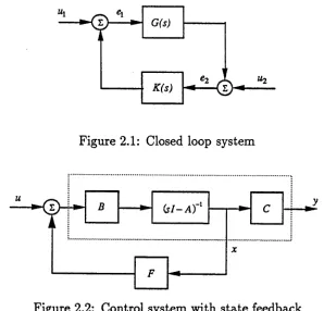
G = C ( s l — A)~XB + D (2.2) The plant G(s) is said to be proper since |G(oo)| is finite. We formally say that a controller K(s) is stabilizing for G (see Fig. 2.1) if the four transfer functions from [u\ u^]' to [e[ e'2}' are stable.

This chapter is concerned with the structure and properties of state es­ tim ate feedback controllers. Unlike much of the work in this area, the state

Chapter 2 Frequency-shaped state estimate feedback 12

G(s)

K(s)

Figure 2.1: Closed loop system

Figure 2.2: Control system with state feedback

feedback gain F and state estimator gain H are here permitted to be proper transfer functions. We recall first what is meant by these terms for the case when F, H are constant. Figure 2.2 shows state feedback for the strictly proper plant G(s) = C ( s l — A)~l B; the feedback signal is Fx(t). The trans­ fer function from u to y is

I jh y = C ( s l - A - B F ) ~ 1B . (2.3)

Chapter 2 Frequency-shaped state estimate feedback 13

that all unstable plant modes will be controllable. If a constant F is replaced by a possibly unstable F (s), then what choices of F(s) will lead to a stable state feedback controller?

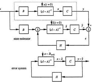
Consider the state estimator in Fig. 2.3, which is the dual of the above case. The transfer function from the input u to the error in the state estimate

x — x is zero, and furthermore, the transient behaviour of this error, due to non-zero initial conditions, will approach zero if H is chosen such that the eigenvalues of A + H C are in the stability region. This is known to be possible whenever the pair (A, C) is detectable, where detectability is equivalent to saying that all unstable modes of A will be observable. If a constant H is replaced by an arbitrary proper transfer function H( s), then what values of

H(s) will give an estimator with an error that tends to zero asymptotically?

Combining state estimation and state feedback, we obtain a state estimate feedback controller. Such a controller, with F, H constant, can be defined

by

x = Ax 4- Bu — H( y — y)

y = Cx -f- Du (2-4)

u = Fx

with transfer function K € R sp

C hap ter 2 Frequency-shaped sta te estim ate feedback 14

state estimator

error system

(si-A)'

C h ap ter 2 Frequency-shaped sta te estim ate feedback 15

This controller is known to be stabilizing if and only if

[si — (A + B F ) } - \ [si - (A + HC )} -1 € R H ^ (2.6)

where RHoo is defined to be the class of proper and stable real-rational transfer functions.

W ith H, F generalized as transfer functions H(s), F(s) £ Rp with sta- bilizable and detectable state-space realizations, the resulting state estimate feedback controller is known to be stabilizing for the plant G(s), with all states asymptotically stable for arbitrary initial conditions if and only if [33]:

F(s), H(s) stabilize Gf, Gh respectively, where

Gf = (s i - A)~l B, Gh = C { sl - A ) ' 1 (2.7)

This result is also shown as a by-product of the theory of this chapter.

In the chapter we show that for the plant G of (2.2) the class of all stabilizing controllers of the form (2.4), parameterized in terms of F, H £ Rv

satisfying (2.7), is the entire class of all stabilizing controllers for the plant (2.2). Moreover, the entire class can be generated in terms of a stabilizing

F £ R P for Gf, where H £ R p is an arbitrary stabilizing controller for Gh

with a left inverse H~ L £ R H ^ . Likewise, in terms of a stabilizing H £ Rv

for Gh, where F is an arbitrary stabilizing controller for Gf with a right

Chapter 2 Frequency-shaped state estimate feedback 16

equivalent to a multivariable generalization of the familiar scalar minimum phase property, with the additional constraint that the transfer function has relative degree zero.

W ith constant output feedback permitted in addition to the state esti­ mate feedback, the class of all proper stabilizing controllers can be generated using a mild variation. In addition, the parameterizations can be in terms of arbitrary transfer functions Qp, Qh € RH<x>, with the closed loop transfer

functions affine in Qp or Qh. The theory developed here is based on re­ sults from factorization theory [46, 11], and complements other work which involves modification to standard state estimate feedback [33, 12].

Chapter 2 Frequency-shaped state estimate feedback 17

estimate feedback. This is not to say that state estimate feedback is always the best design approach, as illustrated when the frequency shaping in the state estimate feedback cancels out the observer dynamics.

In Sec. 2.2, known theory [12, 11] for the class of all stabilizing controllers is reviewed and extended for use in subsequent sections. In Sec. 2.3, the main results of the chapter are developed. Some useful related results are summarized in Sec. 2.4, and conclusions are drawn in Sec. 2.5.

2.2

S ta b ilizin g con trollers for

G, Gf

,

Employing the notation in Appendix A2.1, the transfer functions G, Gf, Gh

from (2.2), (2.7) can be written

A B

C D , Gf

B

, Gh

Jt

A I

C 0_Jt (2.8) Consider also coprime factorizations over R H C

G = N M - 1 = M ~ 1N, Gf = NFM p1 = Mf1N f ,

Gh = N„Mh = 1 Mü' Nh,

where A M ] ? 1, Aifj?1, iWjJ1, MjJ1 €

Let us denote K, F, H€ Rpas stabilizing controllers for Gf, Gh respec­ tively with coprime RHxactorizationsf

K = U V - 1 = V - ' Ü ,

F = UFVf1 = V£xÜf,

H = UhVh1 = Vh' Uh,

where V ~ \ V ~ \ V f l , V f \ V ^ . V J 1 € R p

C h ap ter 2 Frequency-shaped state estim ate feedback 18

Such stabilizing controllers are known to exist with (A ,B ) stabilizable and (A, C) detectable.

For what follows, doubly coprime factorizations of G(s) with respect to the ring RHoo are required. W ith the notation above and

V - Ü ' ' M U ' ' I o '

M N V 0 I

then N M ~ l = provide doubly coprime factorizations of G. With

F, H constant and K equal to the state estimate feedback controller of (2.5), then Nett, Jacobson, and Balas [39] give explicit state space realizations for factorizations of G, K satisfying (2.11).

It is no longer possible to use the doubly coprime factorizations for G of Nett et. al. when F, H are generalized to possibly unstable F (s ), H (s) £ Rv.

Theorem 2.1 overcomes this problem by using suitably modified factoriza­ tions.

T heorem 2.1 Given any F, H £ R p stabilizing fo r Gf, Gh of (2.7) with

factorizations (2.10) and (A, B , C ) minimal, then coprime factorizations for

Gf, Gh, G and K satisfying (2.9), (2.10) are 1;

I. _{'a + b f B V f >'}

= _{F V f 1}

I

0 J

^—Nf A/f]

£ R H C

A + B F - B B F

v f 0 V f 1 e RHC

(2.12)

C hap ter 2 Frequency-shaped sta te estim ate feedback 19

[ Mh ] 'a + h c V '

Nh HC

V

L C

0 J

[ ~ Nh M h ]

M U N V

V

-u

e R H C

A + H C - I H

Vh1C 0 V e R H C (2.13)

A + B F BVf1 - U H

F V f 1 0

C P D F D V f1 V„ _ T

A + H C - B - H D H

Üf VF 0

V„lc

-VZ'D

V

€ R H C

£ RHoo (2.14)

Moreover, the factorizations satisfy the following double Bezout equations:

Vf - Üf ' Mf UF ' ' I 0 '

—Np Mp Nf Vp 0 I

Vh - Uh ' ' Mh UH ' ' I 0 '

- N h _{Mh .} Nh VH 0 I

V - Ü ' ' M U ■ I 0 ■

- N M N V _ 0 I

(2.15)

(2.16)

(2.17)

Proof The properties of (2.9), (2.15)—(2.17) can be verified by simple ma­ nipulations, as shown in Appendix A2.2. It remains to show that the fac­ tors (2.12)-(2.14) are stable, since with (2.15)—(2.17) this implies that the factorizations are coprime in R H ^ . Consider first coprime factorizations

Gf = NfM f1= Ad^A/p. Since F stabilizes Gf, then standard arguments

[46] give that

Chapter 2 Frequency-shaped state estimate feedback 20

Also from (2.15), AIf(Vf — GfUf) = 7, (Vf ~ UfGf) Mf — I so that [MF JVjt] (VF - GfUf) - 1 [I ]

( - M fVF — jVfUf)1 f - V f ' € RH~(2.19) Mf

Nf

I

Gf (Vf - ÜfGf) - 1 A i F

j\fp (VfM f - ÜfX fY 1 e R Hco (2.20)

Analogous proofs for the dual show that Nh, Mh, Nh, Mh € R Hoq. It then follows that N, M, N , M G i?i7oo since

' M ‘ ' I o ' Mp

N D C Np

N M _{[ N}h Mh _{- D}B 0_I

(2.21)

(2.22)

Finally, since F stabilizes Gf, all four closed loop transfer functions are stable. This implies that

[si - (A + B F ) } - \ F[sl - {A + BF) ) ~l B € R H ^

=> F[ s l — (A + B F)]_1 G R Hqo under (A, B) controllable (2.23)

It follows from (2.23) that U, V G R H ^ . Dual arguments show that U, V" G

RHoo.

□

W ith the factorizations of Theorem 2.1 established, then (2.17) implies that [11]:

C hap ter 2 Frequency-shaped sta te estim ate feedback 21

will be stabilizing for G. Other standard results can immediately be applied to G, K based on the doubly coprime factorizations of Theorem 2.1. For instance, it is possible to characterize the class of all stabilizing controllers

K (Q ), th at stabilize G, in terms of an arbitrary parameter Q £ R H <*,.

T h eorem 2.2 ([11, 12]) Consider the plant G of (2.8) with coprime fac­

torizations (2.9), (2.14), (2.17) as above. The class of all proper stabilizing

controllers can be parameterized in terms of arbitrary Q £ R H ^ as

K (Q ) = U(Q)V(Q)~1 = V(Q)~1Ü{Q)

= K + V - 1Q ( I + V - 1N Q )~ 1V - 1

where

U{Q) — U + MQ;V(Q) = V + NQ-, \V + NQ\ ji 0

Ü(Q) = Ü + QM-, V( Q) = V + QN-, \V + Q N \ ^ 0 1 ;

We finish this section with some remarks:

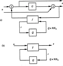
1. The class of all stabilizing controllers of (2.25) can be depicted as in Fig. 2.4, where

J K V - 1 , T =

I - K

- G I ____

i

_ V - 1 - V - ' N

‘ N M 0

(2.26)

2. The closed loop transfer functions are affine in Q,

I - K 1_1

C h ap ter 2 Frequency-shaped sta te estim ate feedback 22

Chapter 2 Frequency-shaped state estimate feedback 23

estimator

Figure 2.5: Class of all stabilizing controllers: Doyle-Stein form

A + H C 0 0 - B - H D - H

B q V j ' C _{a Q} 0 BqVü' D BqVü1

B ( F - DC) BVf' Cq A + B F B ( I + DD) B D

F - D C v f'Cq A + B F I F D D D

D ( F - DC) D V f ' C q C + D F {I + DD)D I a d d

a Q Bq Cq Dq

(2.27) where

D = V f ' D q V j \ Q

--The derivation of T is shown in Appendix A2.2. An alternative de­ piction is in Fig. 2.5; here all stabilizing controllers are be obtained by filtering the residuals r = y — y with an arbitrary Q £ R H ^ , and adding this to the controller output.

3. Observe from (2.25) that given an arbitrary proper plant K\, with arbitrary coprime factorizations

C h ap ter 2 Frequency-shaped sta te estim ate feedback 24

then Qi 6 Rv is uniquely determined such that K i = K ( Q i), since

from simple manipulations:

Qi = —M~l [I — KiG]~l (U — K\ V )

= —[ViM — Ü\N)~l [V\U — U\V]

= - [ U Vl - VUi][MVi - NUi]“1 (2.28)

A consequence is that MQ\ and NQ\ are uniquely determined.

4. Substitution for V, U and V, Ü into (2.17) from (2.25) results in cor­

responding properties for V(Q), U(Q) and V(Q), Ü(Q)

' V(Q) - & ( Q ) ' ' M U{Q) ' ■ / o '

- N M N V(Q) 0 7

With the result (2.29), Ui = U(Qi), V\ = V(Q\), and the duals, then

(2.28) simplifies to

Qi = U{Qi)V - V( QX)U = VU( Ql ) - ÜV( Ql ) (2.30)

5. Note that

[■K ( Q ) G 7?sp] ^ [Q G R-sp] (2.31)

6. Observe that as a consequence of the fact that X2 2 = 0, the transfer

function from e to r is invariant of Q, and is equal to T2 1.

7. With F, H G RH00, then without loss of generality, Vh — I, Vp — /.

In this case, the factorizations of (2.12)-(2.14) simplify to the special­

Chapter 2 Frequency-shaped state estimate feedback 25

8. The above results apply to yield the class of all stabilizing controllers for Gf, Gh in terms of arbitrary Qf, Qh € RH^:

F( Qf) = Vf{Qf)~1Uf(Qf)

= V f l ÜF + VFQF{I + V £ xN FQ F ) - l V f1

Vf(Qf) = V> + QfNf; Üf(Qf) = Of + QfMf ,9 ^

|V> + OfAf| # 0 1 J

and

= UHVSX + Vs 'QhV + Vs 'NhQhY 'Vü1

Uh(Qh) = Uh + MhQh; Vfr(Qtf) = V* + jV*QH

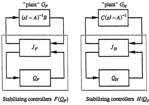
(2.33) Then the transfer functions F (Qf), H( Qh) can be structured as shown in Fig. 2.6, where Jf, Jh are given by

Jf

'-1

F Vp

V f1 - V f ' N p , Jh

- i

H Vj

Vh1 ~ V R 1Nh (2.34)

Chapter 2 Frequency-shaped state estimate feedback 26

"plant" GF "plant" GH

C ( s l - A)'

Stabilizing controllers F(Qf ) Stabilizing controllers H(Qh)

Figure 2.6: Stabilizing controllers F{Qf), H( Qf)

to be defined. It is shown that once the doubly coprime factorizations are established, then standard results on stability can be applied. In particu­ lar, it is possible to parameterize the class of all stabilizing controllers for

G, Gf, Gh- In what follows we show that the class of all stabilizing con­ trollers for G can be achieved by a state estimate feedback controller with dynamic state estimator or state estimate feedback gains.

2.3

S ta b ilizin g con trollers for

G

in term s o f

Q

f

Q

hi

Q

The class of state estimate feedback controllers in terms of F, H G Rp will be denoted as

K [F, h ] = \ A + BF + HC + HDF'a + b f + h c + h d f I - H- H ; j e R ^ (2.35)

C hap ter 2 Frequency-shaped state estim ate feedback 27

Lem m a 2.3 With the definitions (2.35), (2.32), (2.33), and the factoriza­

tions of Theorem 2.1, the following classes of strictly proper controllers pa­

rameterized by QHi QF 6 RHoo are stabilizing:

K[ F, H( Qh )\ = Mh(Qh)Vh(Qh) 1

Mh(Qh) = U + M Qhi Vh{Qh) = V + N Qh (2.36)

K[ F{ Qf)i H] = M Q fY ' Uf{Qf)

Üf(Qf ) = Ü + QfM , Vf{Qf) = V + QFAf (2.37)

where A4, Af, M , Af are given by

A4 U Af V

A + B F 1

1

F 0 0

C + DF Nh Vh \ _T

A + HC - B - H D H'

Of VF 0

- Mf _{- N}f 0 _

e RHC

V

-u

Moreover, the following properties hold

GA4 = Af, M G = Af

e RHC

-1

1 c;« ' M U ' ' M~l M 0

_

- S r

(2.38)

(2.39)

(2.40)

M~l M = - Uf[sI - A - H C ] -xVh1 eRHoo

Chapter 2 Frequency-shaped state estimate feedback 28

Proof See Appendix A2.2

It remains to find conditions under which the class of all strictly proper stabilizing controllers can be structured as K[F, H (Qh)\ or K [F (Qf), H] for Qf, Qh € RHoo.

L em m a 2.4 With the definitions (2.36), (2.37), and (2.25), then

K[F, H (Q h )\ = K (Q ) G R sp & M

N Q G R Sp Q = M 1 M.Qh € Rsp (2.42)

For all Q G RHoo H R sp then there exists Qh G R Ho© satisfying (2.42) if and

only if

F has a right inverse in RHoo (2.43)

(A dual relationship exists for K [F (Qf), H] and K(Q ), the relationship being Q = Q pAdM ~x. The dual of (2-43) involves the existence- of a left inverse

for H .)

Proof See Appendix A2.2. Remarks:

1. Condition (2.43) in Lemma 2.4 is equivalent to specifying that F is a minimum phase transfer function with relative degree zero.

2. Since the closed loop transfer functions are affine in Q, and by (2.42),

Qf is linear in Qh, then the closed loop transfer functions generated

-Chapter 2 Frequency-shaped state estimate feedback 29

3. The results of (2.42) can be generalized by replacing F by F( Qf), for

some Qp £ RHoo. With a fixed F(Qp) and, for example, writing K( Q)

as Hf,h(Q) to denote explicitly the state feedback and state estimator

gains, the (2.42) becomes

K { F ( Qf ), H ( Qh)\ = Kf(qf),h(Q)

Q = - Uf(Qf)[sI-A-HC(2.44)

It follows that the class of all stabilizing controllers can be organized

as K [ F ( Qf) , H ( Qh)]where F ( Qf), H ( Qh) are given by (2.32), (2.33)

and Qf, Qh £ RHoo.

The following theorem is now established from Theorem 2.2, Lemma 2.4, and

their remarks

T h eorem 2.5 Consider the plants G, Gf, Gh of (2.8) with (A ,B )

stabiliz-able and (A , C) detectstabiliz-able, and the state estimate feedback controller K[F, H]

of (2.35) for G.

(i) With F, H € Rp arbitrary stabilizing controllers for Gf, Gh, respec­

tively, then K [F , H] 6 R 3p is stabilizing for G and represents the entire

class of stabilizing controllers for G.

(ii) With Fi £ Rp fixed and (strictly) minimum phase as in (2.43), and

H £ Rp arbitrary stabilizing proper controllers for Gh, the subclass

C h ap ter 2 Frequency-shaped state estim ate feedback 30

frequency-shaped estimator

<2F e RH00 Qh e RH00

Q e RH„

Figure 2.7: Class of all stabilizing state estimate feedback controllers, denoted

K [ F ( Q f ), H ( Qf),Q]

and only if F\ £ R v stabilizes Gf• A dual result holds for K[F,H\\ when Hi is fixed.

As an extension, consider a more general class of state estimate feedback controllers K [F, i7, Q\ as in Fig. 2.7. This is really the class Kf,h( Q ), but writing K[F, H, Q] explicitly shows that there are three parameters F, H, and Q. The class is obtained from the class K[F, H] £ R sp by adding to the controls the residuals (y — y) filtered by Q £ RHoo,

u = Q(y - y ) + F x (2.45)

Chapter 2 Frequency-shaped state estimate feedback 31

the case when F, H are dynamic rather than constant.

T h e o re m 2.6 With the notation above, K [F, H, Q] E Rp is stabilizing for arbitrary F, H stabilizing for Gf, Gh and arbitrary Q E RHoq. Moreover, with Q an arbitrary constant, then K[F, H, Q] represents the entire class of stabilizing controllers in Rp for G.

Proof See Appendix A2.2

□

Remarks:

1. The controllers K[F, H, Q] when Q is a constant, are still conveniently viewed as state estimate feedback schemes with additional output feed­ back. W ith Q constant, then the feedback signal u in (2.45) can be formed as a combination of x and y:

u = (F — Q C)x + Qy (2.46)

When Q is frequency shaped, there is no ready interpretation as state estimate feedback or even frequency shaped state estimate feedback.

C h ap ter 2 Frequency-shaped state estim ate feedback 32

2.4

U se fu l r e la tio n s h ip s

Here several useful formulae will be stated, which relate various transfer functions such as K, Q, J , F, and H of the previous sections. The relation­ ships are verified by algebraic manipulation as was done in Appendix A2.1 for earlier proofs. Consider the plant G with a strictly proper controller

K = C ( s l — Ä)~l B and AT, F constant vectors stabilizing Gjy, Gf respec­ tively. The factorizations (2.14) can then be specialized with Vh = I, Vh — A, Vp = A, and Vp = A. If the control-loop is well posed, then it will be possible to invert (2.25) to obtain a Q such that K( Q) = AT,

Ä + B D C B C B

B C A - H

C - F 0

A + B F + H C + H D F - H B + H D

J = _{F 0 I}

- C - D F I - D

The expression for J is stated in [12]. Also from (2.27),

(2.47)

(2.48)

A + B D C B C B D B

I - K _{B C A} I 0

- G I _{C 0 I 0}

L

(2.49)

Chapter 2 Frequency-shaped state estimate feedback 33

If a constant H is chosen to stabilize C ( s l — A)~l and H has a left in­ verse H~L, then a controller K[F(s), H] can be realized by using a frequency shaped state estimate feedback, with

F{s) =

' Ä + B H - L(B + HD) C - [ Ä + B H - l (B + H D ) C ] B H - L + B H - l (A + HC)

c

(2.50) The dual result exists for K[F, H(s)] in the case when a constant F , which stabilizes ( s i — A)~l B, has a right inverse

Ä + B(C + DF) F~RC B

(A + B F ) F - RC - F - RC[Ä + B( C + DF) F~RC\ - F ~ RC B

(2.51) Note th at existence of a right inverse of the constant H is the same as con­ dition (2.43), but (2.43) considers the case when II is permitted to have dynamics.

2.5

C o n c lu sio n s

Chapter 2 Frequency-shaped state estimate feedback 34

The proofs rely heavily on the structure of the doubly coprime factoriza­ tions introduced in Theorem 2.1, since the derivation of these new factoriza­ tions relies on state estimate feedback theory.

A 2.1

S o m e b a sic d e fin itio n s

S o m e fu n ctio n sp a ces

In this appendix, a few basic concepts will be introduced. The Hardy space

Hqo consists of all complex valued functions G(s) of a complex variable s

that are analytic and bounded in the open right half-plane, IR[s] > 0. The iJoo norm of G(s), denoted 110(3)1100, is defined by

| | G ( s ) | | o o = sup G(s) (2.52)

2Rp]>o

The class R Hqq is a subset of consisting of all rational functions with real coefficients th at are bounded in IR[s] > 0. Alternatively, for a real-rational F (s), then F(s) € R H ^ if and only F is proper (|F(oo)| is finite) and stable

(F ( s) has no poles in the closed right half-plane, R es > 0) . The class of proper functions will be denoted R v\ the class of strictly proper functions, denoted R sp, consists of real-rational functions F(s) for which |jF(oc)| = 0.

Chapter 2 Frequency-shaped state estimate feedback 35

W ork in g w ith sta te -sp a c e rea liza tio n s

Consider a stabilizable and detectable time-invariant linear system G with state equations,

x(t) = Ax(t) -f Bu(t)

y(t) = C x ( t) + Du( t) (2.53) A special notation for the transfer function of such a system will be used,

G{s) = C { s l - A)~l B + D ’a b '

c

The horizontal and vertical lines are not partitioning of the block matrices, but indicate that the matrices represent transfer functions. Using this con­ venient notation, some identities will be given: first for the cascade of two systems, and then for the inverse of a system.

B 1 C 2 B 1 D 2

(2.55)

A \ B! C! D1

A 2 b 2

c2 D 2

A i B \Cs2 B \ D2

= 0 A 2 b 2

T _{. C l D 1 C 2 D l D2}

A B T A - B D ^ C - B D♦

C D _{T . D ' C Dt} (2.56)

with f representing a left or right inverse. The notation can also be general­ ized so that,

C{s)[sl - A (s)]-l B(s) + D(s) =

Two useful matrix identities follow,

A(3)

C(s) D{s) (2.57)

J T

Chapter 2 Frequency-shaped state estimate feedback 36

/ + X ( I - Y X ) - ' Y = ( / - X Y ) ~ l (2.59)

A 2 .2

P r o o fs

D e r iv a tio n o f (2 .9 )—(2.14)

The factorizations (2.9)-(2.14) can be verified. For example

A B F BVf ' ~\ B F

GfMf = o A A B F B V f 1 = 0 A 0 = Nf

.i

ö I ~ J T I

1

n —JT

(2.60) Here the second equality follows from a change of basis (second column added to first column and the first row subtracted from the second row). The third equality follows by the deletion of uncontrollable parts. Similarly, (2.39) follows from definition (2.38) and

1 TA 0 M u 1

(2.61)

GMq =

‘ A B F

0 A + B F - M0 h _

A 0

0 A + B F

Mh - M h

C D F 0 _T C C + DF 0

The properties (2.15)—(2.17) and (2.40) can be proved using similar manip­ ulations based on (2.55).

D e r iv a tio n o f c lo sed -lo o p tran sfer fu n ctio n

Assume that K has the form (2.25), so that K(Q) = U(Q)V(Q)~l where

U(Q) = U + M Q, V(Q) = V + NQ. The closed-loop transfer functions from

u to e in Fig. 2.4 are

Chapter 2 Frequency-shaped state estimate feedback 37

I ~

- G I

- 1

(2.62) Moreover,

I -I<(Q) ' -1 ’ M O ' M —U(Q) '

- G I . 0 V(Q) _ - N V(Q)

- l

M 0

0 V(Q) M M Q '

0 V(Q)

i - Q

0 I M - U - N V

- i

M - U - N V

- i

- l

M 0 ‘ M - U ' -1

+ ' 0 M Q ' ‘ V Ü '

0 V _{. ~ N} V ° N Q _{. &} M

I - G

- K

I +

M

N Q [ N M (2.63)

The result (2.26) follows from (2.63). The state variable form of the closed- loop transfer functions in (2.27) can be derived by substitution for G, K , N, M, N , M into (2.63) from (2.2), (2.5) and (2.17), and with Q = Cq(sI —

Aq) ~ 1Bq + Dq.

P r o o f o f L em m a 2.3

(i) Specializing (2.14) with H = UhV ^ 1 replaced by

H ( Qh) = Uh(Qh)Vh(Qh)~1

of (2.33), and thus U, V replaced by Uh(Qh), Vh{Qh) we have Uh(Qh)

Vh(Qh)

' A + B F —Uh — MhQh

-1 ___________ 1

' M '

Af

= _{F 0} = +

[C + D F Vh + NhQh

T

L ' J

Qh

C hapter 2 Frequency-shaped state estim ate feedback 38

Likewise

[Vf(Qf) - Ü f(<3f)]

A + HC - B - H D H

Vf 4- QfMf Ü + QfNf

o

V -Ü] + Qf [ (2.65)

The class I\[F, H( Qh)] is stabilizing from previous results since F sta­

bilizes Gf and H( Qh) stabilizes Gh• The dual result follows similarly.

(ii) This follows by direct verification as for the derivation of (2.9) and (2.12) in the beginning of the appendix. To show that M ~ l M. € R H0Q, it is necessary to use (2.13)

C[sl - A - H C \ - l V ä l e RHoo n R sp

=► C(A + { HC) [ sI - A - H C ] - 1 + /} € R H „ (by differentiation) = CA[sI — A - H C ] - ' V ü ' + C M „ € R H „

=> CA[sI - A - H C] - 1]/€ R H X (using € R H „ )

Repeated differentiation leads to

[ C (CA)' ■ ■ ■(C 4 "-1)']' [si - A - HC\ ~1V ^ 1 € A#«, n R, p

=>[s/ — A — € R H„fl Rsp (Under (A,C) observable)

C h ap ter 2 Frequency-shaped state estim ate feedback 39

P r o o f o f L em m a 2.4

(i) The second equivalence of (2.42) follows from applying the identities

G M = N and G M = Af. For the first equivalence, compare (2.36) and (2.25), note the property (2.31), and exploit the connections between

Q and K ( Q) as in (2.28) and the corresponding results for Qh and K[F, H ( Qh )].

(ii) Observe that there exists Qh € R H such that

Q — M ~ 1M Qh € RHoo n R sp

Üf[sI — A — HC]~l V ^ l {s + a) has a right inverse in R H ^ (a > Uf has a right inverse in R H ^

F = V f l ÜF has a right inverse in R H ^

T hat is, (2.43) holds.

□

P r o o f o f T h e o rem 2.6

From (2.14), (2.55), and (2.56)

A + B F _{- UH1}- i A + B F + H C + R D F H

C + D F Vh

j

V

(2.66)

and

A + B F + H C + H D F - H C - H D F H D V f 1

V ~ l N = 0 A + B F - B V f

C h ap ter 2 Frequency-shaped state estim ate feedback 40

=

A + B F + HC + H D F B + HD

C + D F D _{-i t} V c l (2.67)

where the last equality follows from a change of basis and the deletion of uncontrolled modes. Likewise for the other terms in J of (2.26), leading to

A + B F + H + DF)- H —( B + H

J = _{F 0}

- V H l {C + DF) V - V i ' D V f '

(2.68)

Applying Theorem 2.2, the class of all stabilizing controllers is of the form of Fig. 2.4, with J as in (2.68). It is straightforward to see that this is of the form K[F, H, Q] as defined in Sec. 2.3. The Theorem 2.6 result follows.

D e r iv a tio n o f r e su lts in Sec. 2.4

The state equations for Q given in (2.47) can be derived by substitution for M , N, U, V from (2.14) into the expression

Q = —(AT - K N ) ~ \ U - K V )

derived from (2.28).

The expression for the frequency shaped state estimate feedback, given a desired controller K = C( s l — A)~l B and constant H with a left inverse

H~L was derived as follows. Manipulations with (2.5) lead to

K = F( s ) ( s l - A - H C ) - \ B I < - H)

Ä B

c 0 F( s ) ( s l - A - HC)

- l

B C B

Chapter 2 Frequency-shaped state estimate feedback 41

It can be verified by direct substitution that one solution for F(s) satisfying (2.69) is

F(s) A B A B

C _{0 . T} BC - H ( . s i - A -HC)

Then (2.51) follows with the use of (2.55)-(2.56) and the identity

(2.70)

C h a p t e r 3

O n t h e e x is te n c e o f s o lu tio n s

o f n o n s y m m e tr ic R ic c a ti

e q u a tio n s

3 .1

I n tr o d u c t io n

Consider the matrix Riccati equations

A T - T Ä - T B C T + BC = 0 (3.1)

ÄZ - ZA - Z BC Z + BC = 0 (3.2)

with T, Z £ Cn,n and A, Ä 6 IRn.n? B 6 lRn,p? B € IRn,g? 0 6 IRg.n and

C € l R p , n

-Although Riccati equations are well studied in the literature there is as

yet no theory giving convenient necessary and sufficient conditions for the

existence of solutions. Potter [41] characterizes all solutions for the symmet­

ric case when A = A*. Other authors [21, 29] give further results for the

symmetric case in relation to the optimal control problem. Clements and

Chapter 3 Nonsymmetric Riccati equations 43

G(s)

K(s)

Figure 3.1: Plant/controller feedback pair

Anderson [9] tackle the problem of factoring a polynomial using the Riccati equation, but with £?, B. C', C' rank one vectors and with A, Ä not necessar­ ily of the same dimension. They give sufficient controllability conditions for solutions to exist.

The results of this chapter were motivated by a problem unrelated to optimal control or spectral factorization. Consider the plant/controller pair of Fig. 3.1 with the following minimal transfer functions,

G(s) = C ( s l — A)~l B (3.3)

I<{s) = C{ s l - (3.4)

where the coefficient matrices are defined as in (3.1), (3.2).