Monte Carlo Methods
Simon Knapp
A thesis submitted for the degree of
Doctor of Philosophy of The Australian National University.
I certify that this thesis does not incorporate, without acknowledgement, any material previously
submitted for a degree or diploma in any university and that, to the best of my knowledge, it
does not contain any material previously published or written by another person except where
due reference is made in the text. The work in this thesis is my own, except for the contributions
made by others as described in the Acknowledgements.
Much of the material in Sections 2.2 and 2.3 was based on work I was heavily involved with while
working at the Bureau of Rural Sciences, and which was done in collaboration with colleagues.
The specific sections are noted in the text. Of particular note, Simon Barry initially conceived of
SPatial REallocation of Aggregated Data Version II (SPREAD II) and Robert Smart prepared
and documented most of the data.
Professional copy editing was provided by Matthew Sidebotham of workwisewords. Finalisation
of this thesis has been far easier since his preening.
Most of the data used in this thesis was generously provided by the Australian Department of
Agriculture and Water Resources. My ex-colleagues there provided interesting insights on the
work presented here and the peculiarities of land use and its analysis in Australia.
The support of my supervisors, and in particular Simon Barry, has been invaluable. His ability
focus on the facts and innovate has been inspirational.
Perhaps most importantly, the work undertaken in this thesis would not have been possible or,
at least, would have beenmuch harder, more time consuming, and of lower quality, had it not
been for the assistance of Robert Smart. He prepared most of the data used herein and has
always had time to chat about, and help resolve, both technical and practical issues.
Finally, I’d like to thank my family. Joanna’s patience and support through what has been
a longer journey than anticipated, one that has taken place alongside starting a family and a
small business, has been extraordinary. As for Alex and Dustin, a main motivator for knocking
We present a flexible, automated, Bayesian method designed for broad scale land use mapping.
The method is based on a Monte Carlo Markov Chain and integrates a number of sources of
ancillary data. It produces a probability density over a finite set of land use classes that can be
used directly in further analyses or to classify individual pixels. The method assumes a
multi-nomial prior over the possible land use types, and uses agricultural statistics to form stochastic
constraints over the total area allocated to each land use within a region. A supervised learner is
then used to allocate pixels within the region, while respecting the constraints. We then extend
this method in three ways. First, supplementary mapping is used to form further constraints
over subsets of the original land use classes. Second, two spatial models are considered; the first
considers the use of partially labelled pixels, where the labels are based on the current state of
the Markov Chain, and the second assumes a Markov Random Field. Third, the form of the
prior is relaxed, and the method extended to allow the creation of a time series of maps using
either cascade or compound classification techniques. The methods are benchmarked against
the probabilistic classifier upon which they are built and simple Bayesian modifications to the
raw classifier that incorporate the same data. The techniques are demonstrated and assessed
using Australian data generated by a national Land Use (LU) mapping program and show
1. Introduction. . . 8
1.1 Background . . . 9
1.1.1 Land Cover and Land Use . . . 10
1.1.2 The Use of Ancillary Data . . . 11
1.1.3 Land Use Mapping in Australia . . . 13
1.2 Outline of This Thesis . . . 15
2. Spatial REallocation of Aggregated Data Version II . . . 17
2.1 Introduction . . . 17
2.2 Methods . . . 18
2.2.1 SPatial REallocation of Aggregated Data (SPREAD) . . . 18
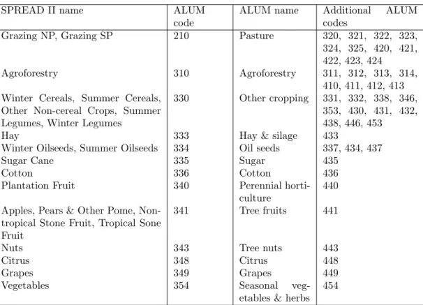
2.2.2 SPatial REallocation of Aggregated Data Version II (SPREAD II) . . . . 19
2.2.3 A Simple Bayesian Classifier . . . 22
2.3 1992–93, 1993–94, 1996–97, 1998–99, 2000–01 and 2001–02 National Land Use Map of Australia (NLUM) . . . 22
2.3.1 Data . . . 23
2.3.2 Running SPREAD II . . . 26
2.3.3 Software . . . 27
2.3.4 Results . . . 27
2.4 SPREAD II Maps for 2005–06 and 2010–11 . . . 35
2.4.1 Data . . . 35
2.4.2 Software . . . 38
2.4.3 Results . . . 40
2.5 Simulation Study . . . 46
3. Including Sub-regional Constraints in SPREAD II . . . 53
3.1 Introduction . . . 53
3.1.1 Possible Approaches . . . 54
3.2 Methods . . . 55
3.2.1 A Single Zonal Constraint . . . 55
3.2.2 Multiple Constraints . . . 57
3.2.3 A Simple Bayesian Classifier . . . 58
3.3 Results . . . 59
3.4 Discussion . . . 61
4. Including Spatial Context in SPREAD II . . . 64
4.1 Introduction . . . 64
4.2 Methods . . . 65
4.2.1 Markov Random Field Approach . . . 66
4.2.2 The Transductive Approach . . . 67
4.3 Results . . . 68
4.3.1 Neighbourhood Size . . . 69
4.4 Discussion . . . 71
5. Producing a Time Series of Maps Using SPREAD II . . . 73
5.1 Introduction . . . 73
5.2 Methods . . . 74
5.2.1 Cascade Classification . . . 78
5.2.2 Compound Classification . . . 79
5.2.3 Transition Matrix . . . 85
5.2.4 A Simple Bayesian Classifier . . . 87
5.3 Results . . . 87
5.4 Simulation Study . . . 91
5.5 Discussion . . . 93
6. Summary and Discussion . . . 96
6.1 Summary of Results . . . 96
6.4 Further Research . . . 105
6.4.1 Applying the Techniques in Concert . . . 105
6.4.2 Producing Maps for Non-Census Years . . . 105
6.4.3 Inclusion of Textures or Objects . . . 105
6.4.4 Incorporation of Multi-resolution Data and Sub-pixel Classification . . . . 106
Bibliography . . . .107
Appendices . . . .115
Continental scale Land Use (LU) information is an important input into many areas of natural
resource management. Examples of areas of current interest include the measurement of land
based Green House Gas (GHG) fluxes induced by LU change (Department of Climate Change,
2009; Australian Greenhouse Office, 2002), agricultural productivity (Bryan and Marvanek,
2004; Marinoni et al., 2012), environmental sustainability (Gardi et al., 2010), food security
(Morrison et al., 2011), and as inputs into biophysical models (Hurtt et al., 2001), health studies
(Maxwell et al., 2004) and salinity modelling (Kiiveri et al., 2003). This broad applicability
and the dynamic nature of the studies to which LU mapping is applicable has rendered it one
of the most widely studied problems employing satellite data (Cihlar and Jansen, 2001).
This thesis considers methods for broad (continental) scale LU mapping using ancillary data
in the form of agricultural statistics and supplementary mapping. The techniques are
demon-strated and assessed using Australian data generated by a national LU mapping program. We
will review the literature on satellite based LU mapping, focusing on studies that have
incorpo-rated ancillary data. We then outline the available LU and Land Cover (LC) data in Australia
and describe the design and structure of this thesis. The methods developed here are
exten-sions to the method currently used for mapping the agricultural components regions within the
The use of remotely sensed data in mapping large areas began in the early 1980s with the
National Oceanic and Atmospheric Administration (NOAA) series of satellites. This was the
first generation of satellites with radiometric sensors advanced enough to be of use for LC
mapping (Tucker et al., 1985; DeFries et al., 1995; Franklin and Wulder, 2002). One of the first
scientific studies reported in the literature that used remotely sensed data for continental scale
mapping is Tucker et al. (1985). This study used Advanced Very High Resolution Radiometer
(AVHRR) Global-Area Coverage (GAC) Normalised Differenced Vegetation Index (NDVI) data
to classify land cover and monitor vegetation dynamics for Africa over a 19-month period. Those
authors note that prior to that study Landsat was the main source of remotely sensed data,
but had not been used to map large regions due to its fine spatial scale and relatively low
temporal collection frequency, which rendered it expensive to process and difficult to use in
automated classification procedures. The high temporal frequency of the AVHRR data allows
for the creation of regular cloud free mosaics and hence the use of classifiers based on temporal
vegetation dynamics. Prior to that work, broad scale maps were derived from preexisting maps
and atlases (Friedl et al., 2002).
Since the original study of Tucker et al. (1985), mapping of large areas has been studied
exten-sively and reviews of the status of the science are published regularly (Loveland et al., 1991;
Franklin and Wulder, 2002; Aplin, 2004). This has been driven largely by the emergence of
global environmental issues such as climate change and biodiversity, which require LU
infor-mation at various scales, and by the broad utility of these data to a wide range of scientific
disciplines (Cihlar, 2000). More recently, technical advances in computational infrastructure,
the advent of high performance and cloud computing systems, and advances in statistical and
machine learning have opened up new research opportunities and increased interest.
The phenomenal increase in computing power and storage space over past decades and the
range and quality of remotely sensed data available have progressively facilitated increases in
the resolution of LU maps. While early broad scale studies were conducted using data with an
approximate 4 or 16km (NDVI GAC or Global Vegetation Index (GVI)) resolution (Loveland
et al., 1991), it is now feasible to produce broad scale maps with resolutions of 1km and below.
For example, the National Land Cover Database (NLCD) covers the conterminous United States
at a nominal resolution of 30m and is produced approximately every five years (Vogelmann et al.,
2001; Homer et al.; Fry et al., 2011; Homer et al., 2015).
Developments in classification techniques used in LU and LC mapping closely follow
develop-ments in machine learning, statistics and pattern recognition. Some of the automated
tech-niques that were being applied at various spatial scales at the time of the work by Tucker et al.
(1985) included maximum likelihood (either Linear Discriminant Analysis (LDA) or Quadratic
Discriminant Analysis (QDA)) (e.g. Townshend et al., 1987; DeFries et al., 1995), principal
components (e.g. Tucker et al., 1985), classification trees (e.g. Lloyd, 1990) and Neural
Net-works (NNs) (e.g. Benediktsson et al., 1990). Since then, techniques such as boosting (e.g. Friedl
et al., 1999; Chi and Bruzzone, 2005), Support Vector Machines (SVMs) (e.g. Bruzzone and
Marconcini, 2009) and variations on those previously considered, which either approximate the
likelihood function numerically or calculate classification boundaries which are less sensitive to
these techniques are themselves computationally intensive and are only now becoming feasible
for large scale studies.
Many of the more recent techniques are based on iterative and/or transductive techniques
(Vapnik, 1998) which exploit unlabelled or partially labelled data, and allow the use of data
from neighbouring time periods (Bruzzone and Marconcini, 2009), and small training samples of
relatively poor quality (Bruzzone et al., 2006; Chi and Bruzzone, 2005). These techniques exploit
the fact that in many thematic mapping applications, the data, and in particular the satellite
imagery, are known for all points of interest a priori and that one is only concerned with labelling
a fixed set of points as opposed to any point in the domain of the spatial imagery or some
metrics thereon. This allows transductive techniques to exploit information in the observations
to be classified, as well as that in the training data. These are important developments, as
one common problem faced by LU and LC studies is the scarcity of good quality training
data that are representative of the classes being mapped and can capture correlations between
observations that are close spatially and/or temporally (Bruzzone et al., 2006).
1.1.1 Land Cover and Land Use
While LC can theoretically be defined precisely at a given point in space and time, the
appro-priate LU label to apply to a given LC will vary with the purpose for which a map is being used
(Cihlar and Jansen, 2001) and appropriate taxonomies for both LC and LU must be defined
with respect to a specific ontology or purpose of a map. For example, Matsuoka et al. (2007)
produced a map primarily for use in hydrological modelling of the Yellow River in China;
con-sequently the LC classification is focused on separating classes of primary importance to water
flows. In contrast, and due largely to their expense, most broad scale mapping projects aim
to produce classifications designed to be useful for a wide range of analyses, either directly or
through reclassification appropriate to the goals of a specific project. Reclassification usually
involves grouping of classes or disaggregation using ancillary data. These large scale studies
also aim to create products enabling the comparison of LC and/or LU over broad regions or
be-tween regions, or consistent inputs to global climatological or biophysical models (Bartholom´e
and Belward, 2005; Cihlar and Jansen, 2001; Loveland et al., 1991).
The methods used in mapping LU and LC can differ. Since LU is more an anthropological
issue (Cihlar and Jansen, 2001; W¨astfelt, 2009), it is possible to map some LU classes in some classification schemes based on administrative boundaries, cadastres or other spatial datasets.
This is the case for the production of the NLUMs, in which all non-agricultural LUs are derived
directly from administrative boundaries. LC, on the other hand, can change in response to a
wide range of climatological and environmental factors beyond the control of man and hence is
generally determined through data analysis or surveys. LC is also much more sensitive to scale.
For example, at a broad scale a LC might becommercial forest, but at a finer scale subregions
within a commercial forest may be (perhaps in a different classification scheme)bare ground or
pine forest.
Where LU cannot be mapped from administrative boundaries or the like, it is generally inferred
from LC. Consequently, most broad scale mapping projects involve some element of LC mapping
While the techniques explored in this thesis were developed for the classification of LU, they are
equally applicable to LC. Further, some of the LU classes contained in the target classification
schemes essentially map to a specific LC when considered over a single year (e.g.
agroforestry, citrus,apples, grapes andnuts), while many others may encompass multiple LC
classes (e.g. seasonal cropping and pastures in crop/pasture rotations). In the latter case,
we would hope that the variety of LC combinations that occur within a given LU class are
represented in the training data. In any case, due to their increased heterogeneity, it is likely
that mapping such classes will be more difficult without relatively large amounts of training
data that is geographically close to the region being mapped unless the LC sequences vary little
spatially.
1.1.2 The Use of Ancillary Data
Over large regions, limitations in the availability of observational and training data become
more pronounced, and climatological and/or other environmental conditions may increase
het-erogeneity of observed data within an individual LU or LC, hence reducing the accuracy of
classifiers. Further, large scale mapping projects generally use relatively coarse scale remotely
sensed imagery due to the expense, availability, low collection frequency and computational
difficulties associated with obtaining and processing the large volumes of fine scale imagery
that would otherwise be required. Individual pixels within coarse scale imagery often contain
multiple LUs or LCsand the accuracy of classifiers is likely to be decreased relative to finer scale
imagery.
Classification methods that only use remotely sensed imagery are generally not sufficient for
discriminating between LU or LC classes due to both similarities in the reflectance spectra
from various LUs or LCs (Bryan and Marvanek, 2004; Kiiveri et al., 2003; DeFries et al., 1998;
Jewell, 1989). Technical issues with the collection of the data such as intertemporal and spatial
climate variability, disturbance events (e.g. fires and land management), sensor conditions (e.g.
view angles and sensor calibration drift) and signal contamination (e.g. atmospheric
contami-nation and soil color) (Lu et al., 2003) also reduce the discrimicontami-nation power of remotely sensed
imagery. These issues are particularly problematic when there are a large number of classes in
a classification scheme, as is case in the work undertaken in this thesis.
To deal with these issues, broad scale mapping projects tend to depend on highly sophisticated,
automated algorithms that incorporate ancillary data in order to improve discrimination and
reduce labour costs (Richards et al., 1982; Rogan et al., 2003). Techniques for including
ancil-lary data range from expert opinion being applied post hoc (e.g. Loveland et al., 1991) through
to fully automated techniques based on training data (e.g. Melgani and Serpico, 2002). Aplin
(2004) and Franklin and Wulder (2002) review this research and provide references to particular
studies. Sources of ancillary data that have been used in LU and LC mapping include other
satellite imagery collected over the region of interest, information on landforms (e.g. elevation,
slope and soil type information), expert knowledge, administrative data, official statistics,
bio-physical models, classifications at other time periods and other classifications at the same time
One important source of ancillary data used in LU and LC mapping generally, and central to
the methods explored in this theses, is Agricultural Statistics (AgStats), which give estimates
of the total area within a region being used for each LU. These data provide direct estimates
of quantities of interest, albeit at a generally broad spatial scale, which complements the
rel-atively fine-scale contextual data provided by remotely sensed imagery (Bryan and Marvanek,
2004). Most methods reviewed in the course of this thesis incorporate these data through post
hoc calibration procedures which lack theoretical foundations and/or make strong assumptions
about the extent to which relationships between LUs hold between regions. Several methods
that rely on AgStats and demonstrate the types of techniques used to incorporate them are
described below, and Kuemmerle et al. (2013) provide a review of more recent studies in the
context of LU intensity mapping.
Ramankutty and Foley (1998) reclassify the DISCover LC dataset (Loveland et al., 1999) into
six classes that are each assumed to have a globally homogeneous fractional crop cover. They
then systematically assign a fractional crop cover to each class; use linear regression to compare
the resulting weighted sum (an area) to the area of cropping reported in various AgStats data
within each political unit; and choose the set of fractional crop cover that yields the highest
correlation coefficient such that the estimated slope is between 0.9 and 1.1.
Khan et al. (2010) use the ISODATA algorithm (Ball and Hall, 1965) to cluster pixels based
on their temporal NDVI profiles, then use linear regression to relate AgStats, (the dependent
variable) to the area of each cluster type, (the explanatory variables) within a region, one crop
type at a time. For each crop type, the estimated coefficients for cluster type are interpreted
as the fraction of a cluster of type that is being used for that crop type. Biggs et al. (2006) use
the same approach for LU typesirrigated using surface water,irrigated using groundwater and
non-irrigated.
Hurtt et al. (2001) also use the DISCover dataset and estimate the composition of the LU
classes defined in the AgStats in terms of the LC types of the DISCover. They use a multiple
response regression of the formc=Ar, wherecis a vector (of length 4) of areas of various LU
types based on AgStats data,ris a vector (of length 16) of areas of various LC types based on
the LU classes from the DISCover data, andAis a matrix (of dimension 4×16) of fractional
covers.
Maxwell et al. (2004) use areal estimates of corn harvest to choose training pixels that are likely
to be corn. After measuring the spectral distances between the training pixels and all other
pixels, they label each pixel ashighly likely to be corn, likely to be corn or unlikely to be corn,
such that the combined area of the pixels labelled highly likely to be corn is 75 percent of the
area of corn according the areal estimates, the area of likely to be corn is the remaining 25
percent, and the remaining pixels are labelledunlikely to be corn. These percentages werebased
on a sensitivity analysis performed on the three test counties through a trial and error process.
Frolking et al. (2002) use sown area of each crop and total crop area (the combined sown area
of all crop types) estimated from AgStats data along with a set ofMulticrop Rotation Priorities
in an iterative procedure to determine the proportion of area within subregions that is under
one of several crop rotation regimes. They combine this data with a fine scale LC database
derived from Landsat TM data that includes categories ofrice paddiesandnonflooded cropland
provinces using an auxiliary variable that is reported at both scales. Aalders and Aitkenhead
(2006) use neural networks, Bayesian networks and regression trees to demonstrate that a range
of social variables reported in an agricultural census can be used to assist in LU mapping.
W¨astfelt (2009) presents a method for post-classifying a LC map developed from an unsuper-vised classification algorithm into a LU map. The method encodes the spatial configuration
of the LC within a study area of known LU through maximum nearest-neighbour distances.
Other regions can then be re-classified based on the similarity of their LC configuration based
on the same unsupervised learning algorithm to that of the study region. A similar method is
presented in Chen (2002), who uses homogeneity metrics to separate urban density based on a
method using the spatial context of a pixel to help determine the LU of that pixel. By
intro-ducing the spatial context, they demonstrate that it becomes possible to distinguish different
LUs, even when the spectral profiles of these pixels are very similar.
Two methods that incorporate the AgStats data into the primary classification procedure are
You and Wood (2005) and Walker and Mallawaarachchi (1998). You and Wood (2005) seek to
estimate the proportion of each pixel that is used for each of a set of crop types within a set
of pre-defined “production systems” by using linear programming to minimise the cross-entropy
between these proportions and ‘prior’ estimates thereof, subject to a range of constraints.
Pro-duction systems partition the space of possible proPro-duction techniques with respect to equipment,
inputs (e.g. chemical and mechanical) and plant varietals (e.g. high/low yield). The priors are
developed from any available data, including: production statistics, land use data, satellite-based
land cover map, biophysical crop ‘suitability’ assessments, population density, distance to urban
centers and any prior knowledge of crop distribution (You et al., 2009). The data are combined
into the prior using practical methods that suit the specific forms of data. The method also
requires estimates of the total proportion of the total physical area of each crop type within
each production system. The authors adapt and extend this approach in You and Wood (2006)
and You et al. (2009) by incorporating various other data sources.
The second method is that of Walker and Mallawaarachchi (1998), which presents the algorithm
SPatial REallocation of Aggregated Data (SPREAD). This is a linear programming algorithm
that allocates a LU to each pixel within a region while ensuring that the total area of each
LU is equal to that reported by the Australian Bureau of Statistics (ABS) AgStats for the
corresponding time period. This method is discussed further below.
1.1.3 Land Use Mapping in Australia
Here we review the continental scale LU and LC products available in Australia and describe the
context for how some of the methods considered in this thesis could contribute to the Australian
national mapping system through the NLUM.
Australia has two existing continental LU products and one continental scale LC product,
each of which serve different purposes. The LU products are the Catchment Scale Land Use
Map of Australia (CLUM) (Department of Agriculture, Fisheries and Forestry, 2014) and the
NLUMs (Stewart et al., 2001; Smart et al., 2006). The LC product is the Dynamic Land Cover
Dataset (DLCD) (Lymburner et al., 2010), which provides continental scale information and has
The CLUM is effectively a high resolution ongoing census of LU across Australia. This data
is used extensively for Natural Resource Management (NRM) evaluation and activities such as
water quality, soil erosion and acidification (Australian Bureau of Agricultural and Resource
Economics, 2011). The data is collected by various state government agencies across Australia,
with regions being updated as new data becomes available. While detailed, the currency of the
CLUM varies spatially and at any one time varies by around a decade. Consequently, it has
limited utility for analyses that require regular ongoing measurement of a phenomena, such as
GHG emissions or modelling with a temporal aspect. Data collection is largely manual and the
methods used differ between agencies and hence spatially. While the data is presented nationally
using a consistent classification scheme (the Australian Land Use and Management (ALUM)),
since LU is somewhat subjective and the data is collected and prepared by a diverse group of
individuals working for different agencies, it is likely that there will be coding discrepancies
between jurisdictions. The resources allocated to the CLUM also vary between agencies and
consequently, there are regional differences in the level of accuracy. The required attribute
accuracy of these data is at least 80 percent (Australian Bureau of Agricultural and Resource
Economics, 2011). We use the CLUM data in the current work for validation of our results in
selected regions where the currency aligns.
The NLUMs provide a time series of LU maps of Australia with each map corresponding to a
twelve month period. These are at a coarser resolution and are less accurate than the CLUM.
They are much cheaper to produce, as described below, and the same (repeatable) methodology
is applied across the entire continent and (more or less) to each time period. These data are
used for “synoptic-level land use assessments, and for strategic planning and evaluation (such
as setting regional investment priorities and developing programs for natural resource
manage-ment). They are also used in modelling applications, such as national carbon accounting and
salinity assessments at the river basin level.” (Australian Bureau of Agricultural and Resource
Economics, 2011). To date, national maps have been produced for the financial years 1992–93,
1993–94, 1996–97, 2000–01, 2005–06 and 2010–11. Presently a new map is prepared for every
agricultural census year, which, since 2000–01, is every five years. The NLUMs are published
using the ALUM classification and all non-agricultural LUs determined deterministically from
administrative datasets (i.e. only agricultural LUs are estimated statistically).
The Dynamic Land Cover Dataset (DLCD) (Lymburner et al., 2010) is a LC dataset produced
by clustering pixels based on summary metrics extracted from Moderate Resolution Imaging
Spectroradiometer (MODIS) Enhanced Vegetation Index (EVI) 250m data for an eight-year
period, followed by a post-classification step that combines a range of other datasets and expert
opinion. While this is an LC dataset, some of the classes correspond directly to LU classes
mapped in the CLUM and NLUM datasets: specifically,irrigated cropping andrain-fed
(non-irrigated) cropping, pasture and sugar. Since these, in particular cropping and pasture, are
extensive in most agricultural regions, there should be a reasonably strong link between this
dataset and those mentioned above. The accuracy of the DLCD dataset is reported using afuzzy
logic system(Zhang and Foody, 1998), which reports matches at different levels of accuracy. The
reported match rates against field validation sites areexact: 30 percent, very similar: 35 percent,
moderately similar: 10 percent, somewhat similar: 18 percent and completely mismatched: 7
percent.
or DLCD are not. One of the benefits of the methodologies used in compiling the NLUM, is
that they preserve the regional total reported in the agricultural censuses and hence provide
protection from serious error at the regional scale. This is important for applications such as
GHG reporting, as the regional and national totals are of prime importance for international
reporting requirements. Further, being derived from censuses, the regional totals are likely
to be relatively accurate. It is also important for many modelling applications which aim to
produce a time series of information related to LU. Stewart et al. (2001) describe many actual
and potential applications to policy, regulation, NRM etc. of the NLUM data.
Analysis of the relative costs of producing the NLUM and CLUM was done in Stewart et al.
(2001). They estimated that the cost of production of an NLUM was between 3.3 and 12.5 cents
per km2, while the cost of detailed mapping, based on similar approaches used in collecting
CLUM data, was around 50 cents per km2. It should be noted, however, that the NLUMs
incorporate information from the CLUM data and their accuracy would be reduced without
those data. Hence, the cost of producing an NLUM of similar quality would be higher without
the CLUM data.
1.2
Outline of This Thesis
The work undertaken in this thesis is motivated by spatially consistent, repeatable, continental
scale LU mapping, using agricultural classification schemes that contain in the order of 20
to 40 LU classes, in a manner in which the outputs accurately reflect uncertainties. The
techniques employed must be highly automated in order to minimise labour costs, avoid spatial
inconsistencies that could be introduced by analyst intervention, and allow for regular updates.
Of the methods reviewed above, the methodology underpinning SPREAD, which is a highly
automated technique that was designed for use with the same data we have available, is the
most appropriate starting point. The methodologies underpinning the other methods are not
suitable for one or more of the following reasons: they do not propagate uncertainties through
to the outputs, require manual intervention or interpretation on the part of the analyst, are
designed for simpler classification schemes, cannot readily be extended to include additional
data sources, are targeted and much less complex classification schemes, pertain to spatial
partitions other than rasters, or use input data which is unavailable (at acceptable cost) at a
national scale.
As discussed previously, at geographic scale and complexity of classification scheme considered
herein, remotely sensed imagery alone are not sufficient for mapping the LU. Hence, classifiers
used for this type of mapping need to incorporate other sources of information in order to
dis-criminate effectively between LUs. We would like the methods we develop here to be relatively
easy to modify to incorporate new data sources as they identified or become available.
We present a Bayesian method that incorporates a probabilistic classifier with regional estimates
of the area of land used for various LUs, which we refer to as “areal constraints”. The prior
used by this method takes the form of a categorical distribution over the possible LU classes at
each pixel and the posterior is categorical over the same set of classes. We then present a series
spatial/temporal relationships between neighbouring pixels or time points.
In the second chapter we present SPatial REallocation of Aggregated Data Version II (SPREAD II),
the algorithm developed for the production of version 3 of the NLUM. This is contrasted to
SPREAD, which was used to produce versions 1 and 2 of the NLUM. We explore the
perfor-mance of SPREAD II on a study region, by comparing its results to the CLUM and to SPREAD.
We conduct a simulation study to ascertain its robustness to biases in the areal constraint data
with respect to noise in the satellite imagery. In both these analyses we compare it to ‘simpler’
classifiers which incorporate the same inputs using different methodologies.
In the third chapter we introduce another source of ancillary data, in the form of a digital
map that specifies regions where certain groups (which we refer to as “super types”) of LUs
occur, and contrast the results with those obtained in the second chapter. Such data are often
cheaply available from other industry-specific or regional studies and provide valuable
informa-tion that we would like to exploit. Indeed, for some LUs such data are taken as deterministic
in the production of the NLUMs when the LU is unambiguous; for example military areas and
national parks. The challenge addressed in Chapter 3 is to leverage such data when it is not
deterministic. Our experience in producing version 3 of the NLUM suggested that this will
improve classification performance regardless of the quality of the satellite imagery.
In the fourth chapter we evaluate two methods for including spatial context. The first of these
methods is based on Markov Random Fields (MRFs) and should improve our results if pixels of
the same LU are clustered spatially. It is unlikely that this will improve classification accuracy
for LUs that occur with spatial extents smaller than that of the satellite imagery being used,
but may benefit broad scale LUs. The second method is a transductive technique designed to
exploit local similarities in climatic conditions, seasonality, phenology, management and other
factors that affect the spectral signature of specific crops spatially. Both of these methods are
only likely to improve classification performance if the satellite imagery is informative in its
own right.
In the fifth chapter we explore making a sequence of maps. Both compound and cascade
classifiers are introduced and trialled with and without transition probabilities (a matrix of
probabilities specifying the probability that each LU will ‘transition’ to itself or some other
between two time points). In the work here we develop the transition matrix from regional
statistics published by the ABS and discuss the limitations of this approach. Once again, these
methods are only likely to improve classification accuracy if the satellite imagery is informative
in its own right.
In the sixth and final chapter, we summarise the results from a number of study regions, discuss
2.1
Introduction
This chapter considers a new approach to the incorporation of regional statistics in LU mapping,
SPREAD II. This method combines information on crop types from AVHRR NDVI satellite
data with regional statistics providing estimates of the area of land within a region is used for
each of the LUs being mapped. We refer to these data as “areal constraints”. The areal
con-straints used here are derived from AgStats data published by the ABS. The background theory
underpinning SPREAD II is briefly described in Bureau of Rural Sciences (2004, Appendix 7),
but is restated below for convenience and because this method provides a starting point for the
developments considered in this thesis.
A wide range of remotely sensed data is available for pixel classification and a great deal
of work has been done on the development and selection of appropriate data and classifiers.
The methods explored in this thesis assume that the remotely sensed data and the underlying
probabilistic classifier used to estimate [Yi|Ci =k], where k is a specific LU label, Yi is the remotely sensed data available at pixel i and Ci is the LU of pixel i, have been chosen. We also assume that all data have been registered and cleaned; that is, we do not address issues
related to the preparation of the remotely sensed data, the choice of ‘primary classifier’, or any
other data used in the classification process beyond describing the specific data we have used
and how they have been prepared.
The SPREAD II approach addresses shortcomings of SPREAD that were identified when
pro-ducing version 1 of the NLUMs. It allows for the integration of both AgStats data and other
forms of ancillary data with the outputs of an existing probabilistic classifier and the posterior
distribution provides a meaningful measure of uncertainty.
We consider three sets of analyses. The first considers regions that were used in earlier versions
of the NLUM. The results presented for these regions are based on version 3 of the NLUMs.
It is presented here to allow comparison with SPREAD. The second set of analyses consider
more recent time periods. The third set of analyses are based on synthetic data. These analyses
are important in understanding when SPREAD II does and does not perform well and how it
compares to ‘simpler’, less computationally intensive classifiers under various scenarios.
Section 2.2 presents the SPREAD II methodology, which we refer to hereafter as “vanilla
SPREAD II” to distinguish it from variants that incorporate other ancillary data or techniques
data as presented in other chapters. We also present an overview of the SPREAD methodology,
noting some deficiencies identified during the production of version 2 of the 2000–01 NLUM.
com-pares the outputs of SPREAD II to those of SPREAD and the CLUM. Section 2.4 presents
the methodological differences and the data used in the work presented here and Section 2.4.3
compares these results to the CLUM. Section 2.5 presents and discusses the simulation study
and finally, Section 2.6 summarises the results of this chapter.
2.2
Methods
A map comprises of a number of regions. A region is a lattice ofN pixels that we will generally index by n. There are K LUs that we will index by k and pixel n has an actual LUCn ∈ {1, . . . , K}. Here, a region is a reporting region for the AgStats. The total number of pixels with LUkis
Tk = N X
n=1
I(Cn=k), (2.1)
where I(a=b) is the indicator function taking the value one if its argument is true and zero otherwise. We use bold notation to represent the vector version of arguments over their natural
dimension. For exampleT= (T1, . . . , TK), i.e. over the indexk.
The aim of the inference is to inferC, the LU of all individual pixels. We haveM measurements Yn = (Y1n, . . . , YM n) for each pixel, and a sample of locationsj = 1, . . . , H where the LU is known, which we shall refer to as control sites. In our work to date with both SPREAD and
SPREAD II, Yn are fortnightly or four-weekly NDVI values based on NOAA-AVHRR data
over a twelve month period (see Ramsey et al. (1995) for example).
2.2.1 SPatial REallocation of Aggregated Data (SPREAD)
SPREAD performs the above inference using a linear programming algorithm that disaggregates
LU within a region while ensuring that the total area of each LU is equal to that reported by
the ABS AgStats for the corresponding time period. It was used in Stewart et al. (2001) to
produce version 1 of the NLUMs. While Walker and Mallawaarachchi (1998) consider a range
of practical issues in the generation of LU maps (such as non-coincident target and statistical
zones and pixels of mixed LU) in their presentation of SPREAD, we will focus on the core
scientific basis of the technique.
The Gower metric (Gower, 1971) between thenth pixel and thejth control site is given by
gnj = 1 |Sk|
X
s∈Sk
|Ysn−Ysj|
Range(Ys), (2.2)
whereSk is the set of all control sites with LUkandYsis the set of measurements of the sth variable in the entire dataset (i.e. all control sites and pixels).
The SPREAD algorithm assumes thatT is known and fixed. It seeks to allocate the LUs to
the pixels to form predictions ˆCn such that the areal constraints given by equation (2.1) are satisfied and the objective function
G= N X
n=1
K Y
k=1
hI( ˆCn=k)
nk j∈Sk nj
SPREAD is a novel and significant research achievement but exhibits a number of statistical
flaws that became evident while using it to produce the 1996–97 NLUM (Stewart et al., 2001).
These are as follows:
1. The algorithm cannot incorporate uncertainty in the AgStats (T). This is an important
issue as administrative records are rarely without error. We note that in the periods
considered herein, the AgStats are based on censuses and hence the error is hard to
quantify, but if the methods were applied to survey (as opposed to census) data, the
estimates will contain, potentially significant, sampling error.
2. The algorithm is an optimisation algorithm and not a statistical model or framework and
hence does not provide a framework for estimating and expressing uncertainty arising from
uncertainty in the inputs and the estimation process in its outputs. In practice there is
considerable ambiguity in the classification of pixels due to failures of assumptions (e.g.
pixels of mixed LU) and limitations in the ability to discriminate between LU classes.
3. The classifier based on the Gower metric is inefficient. This metric defines a geometry
that may not discriminate between the LUs effectively. As an extreme example, if a single
measurementshas all the discriminatory power, the other measurements simply add noise and could swamp this information. The authors note, however, that it “could be replaced
with any of the measures commonly used in supervised classification of imagery”.
SPREAD II attempts to address these problems by using a very different approach that
al-lows assessment of uncertainty, incorporation of a any probabilistic classifier and extension to
incorporate of a wide range of ancillary data of varying forms.
2.2.2 SPatial REallocation of Aggregated Data Version II (SPREAD II)
Vanilla SPREAD II is based on the same data as SPREAD and uses an Markov Chain Monte
Carlo (MCMC) algorithm to produce a posterior probability distribution over the various
agri-cultural LU classes for each pixel.
LetΘbe a vector of parameters and [•] denote a density function or probability. The algorithm
uses a categorical prior over the various LUs that occur within a region at each pixel within the
region. We denote the parameters of these priors with Π. As described below, in the vanilla
form presented here it is important that categorical prior be the same at every pixel. The
posterior distribution integrates the AgStats data with the outputs of a probabilistic classifier
[Yn|Cn] using the conditional distribution [T|Θ] as a stochastic constraint. A ‘final allocation’
(a single layer map) is then produced that maximises the posterior mean while respecting the
areas reported in the areal constraint data.
The joint distribution of the parameters and data in SPREAD II is:
[C,T,Y,Θ,Π]. (2.4)
full conditional distribution [Ci,T|C−i,T−i,Y,Θ,Π], where C−i is C with Ci excluded and T−i isTcalculated excluding Ci. This can be decomposed as
[Ci,T|C−i,T−i,Y,Θ,Π]
∝[Yi|C,T,Θ,Π][C|T,Θ,Π][T|T−i,Θ,Π][T−i,Θ,Π] ∝[Yi|Ci][C|T,Π][T|Θ]
∝[Yi|Ci][Ci|Π][T|Θ] [T|Π] .
(2.5)
Here we have asserted that the pixels are independent, the satellite imagery for a pixel depends
only on the LU of that pixel and that the LU of a pixel is independent ofΘgivenT. We treat
ΘandΠ as constants and hence [T−i,Θ,Π] is constant for allCi∈K and can be ignored.
We work with areas rather than pixel counts by substituting [A|Θ] for [T|Θ], where A is a
vector of areas allocated for each of the LUs. The area of pixelnisan.
The terms in (2.5) are quite general and, provided the conditional dependence is respected, a
wide range of models could be used for each. We have used:
• [Yi|Ci] is estimated using a kernel density smoother from metrics calculated from the temporal NDVI profiles of the control site; specifically: the mean, range and time of year
of the maximum NDVI value. These metrics are very similar to those chosen in DeFries
et al. (1998) except we use time of year of maximum NDVI, which is subject to seasonality
and hence not meaningful in the context of global study such as theirs.
• [Ci = k|Π] = 1/K ∀ k ∈ {1, . . . , K}, and hence [C] is the constant 1/KN and [T] is multinomial.
• Θ is a constant vector of length K containing estimates, based on the AgStats, of the area of each LU (in hectares).
• [A|Θ] is multivariate normal with a mean vector [µ1, µ2, . . . , µK] and a diagonal K×K
covariance matrix with diagonal entries [σ2
1, σ22, . . . , σK2]. In the published versions of the NLUMs produced to date and the current work, σk = 200 (hectares).
When these terms are substituted into (2.5) we get
[Ci,T|C−i,T−i,Y,Θ,Π]∝
[Yi|Ci=k]( ˜Tk+ 1)φ( ˜Ak+an;µk, σ2k) φ( ˜Ak;µk, σ2k)
(2.6)
where an is the area of the pixel under consideration and φ(x;µ, σ2) is the normal density function with meanµand varianceσ2. Quantities with a tilde represent values before the new
LU is selected (i.e. excluding the current pixel).
Note that (2.6) does not depend on Π. This occurs because [C|Π] in the numerator of (2.5) cancels with the product of probabilities in the multinomial distribution in the denominator
and implies that all prior information must enter the model through the constraints. This is
computationally convenient, but restrictive, as one could introduce all kinds of data into the
the specification that they be the same for all pixels is required to make (2.5) tractable. In full
generality [T|Π] is
[T] =X S
N Y
n=1
K Y
k=1
πI(Cn=k)
kn ,
whereπkn is the probability that pixelnhas LUkandSis the set such that (2.1) holds for all k∈K. The cardinality ofSisN!/T1!T2!· · ·Tk!. If, however, each pixel has the same categorical prior (that is [Ci =k] =πk), then [T|Π] is multinomial and easy to work with. We present an approximation in Chapter 5 in the context of producing a sequence of maps that could be used
to remove this restriction, but do not pursue this further here.
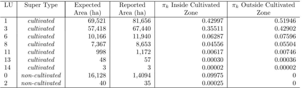
When producing version 3 of the NLUMs we added further constraints, based on spatial data
describing zones where irrigation and horticulture occur. LettingS be the total area of agri-cultural land inside the irrigation zones,AI be the total area of land allocated to irrigated LUs inside the irrigation zones,αbe the mean proportion of the total area of agricultural land inside the irrigation zones that is used for irrigated LUs, andσ2be the variance of the constraint, we multiply (2.5) by
φ(AI;αS, σ2).
An analogous expression is used for the horticulture zones and the complementary non-irrigation
and non-horticulture zones.
This modification was introduced to deal with horticultural crops being allocated where they
were known not to occur. The introduction of these terms is based on a heuristic argument, as
[T] is no longer a simple multinomial distribution. This issue is resolved in Chapter 3.
Through the running of the MCMC algorithm, counts of how many times each pixel is allocated
each LU (ckn) are maintained. Once the algorithm has completed, the posterior probabilities of each pixel having each LU are calculated using the posterior mean of the sample,
ˆ πkn=
ckn
R , (2.7)
where R is the number of iterations (excluding burn-in) for which the MCMC algorithm was run.
The Gibbs sampling algorithm produces a distribution of maps (i.e. updates sufficiently
sepa-rated in the sequence can be taken as samples from the joint posterior of the pixels). While this
is attractive theoretically, users generally want a (single layer) thematic map. An issue that
has been noted of Bayesian approaches is thatproportional prior probability may be used; but
in this case large classes tend to be overestimated and small classes are underestimated or even
disappear (Carfagna and Gallego, 2005). This was also raised by Strahler (1980). This was
our initial experience with SPREAD II when producing a thematic map from the posterior. In
order to combat this, we apply Algorithm 1 which successively chooses the least abundant LU
class, as reported in the to the AgStats, and allocates that class to the pixels with the highest
posterior probabilities for that class. This process is then repeated on the remaining LU classes
until all pixels are allocated. This was chosen as a practical approach and ensures that the
final allocation map is consistent with the agricultural statistics at the regional scale. This is
may also make the map more appropriate for uses which are concerned largely with regional
totals as is often the case for planning purposes.
Algorithm 1Final allocation Algorithm
1: Create a list of all pixels in the region being classified.
2: Sort this list in descending order based on the probability value for the rarest LU.
3: Allocate the firstmpixels such that area constraint for the rarest LU is satisfied and remove the allocated pixels from the list.
4: Repeat steps 2 and 3 until all pixels are allocated.
This describes the mathematical foundation of SPREAD II. Some implementation details are
given in Section 2.3.2.
2.2.3 A Simple Bayesian Classifier
The probability model (2.4) is a generalisation of:
[C,Y,Θ,Π] = [Y|C][C|Π][Π,Θ]
= N Y
n=1
[Yn|Cn][Cn|Π][Π,Θ],
(2.8)
in which the second line assumes that the LU class of a pixel is independent of those of the other
pixels. A relatively early appearance of this in the context of “maximum likelihood classification”
(specifically QDA) is Strahler (1980). A simple way of incorporating the AgStats data into the
classification is to let [Π,Θ] be degenerate and
[Cn =k|Π] =πnk=πk= µk
A.
That is, the prior probability of a pixel having LUkis the proportion of all (agricultural) land (A = PK
k=1µk) that has (agricultural) LU k according to the AgStats. This corresponds to [Ci=k|Π] =πk and [T,Π,Θ] being a multinomial distribution over the counts of pixels with each LU in (2.5). We present results for this model for comparison with the vanilla SPREAD II.
We also present results for SPREAD II with σk2 = Aπk(1−πk), which corresponds to the variance ofTk under the corresponding multinomial distribution. This will provide insight into the impacts of ignoring the off-diagonal elements of the covariance matrix when we compare it
to this ‘simple’ Bayesian model.
2.3
1992–93, 1993–94, 1996–97, 1998–99, 2000–01 and 2001–02 National Land
Use Map of Australia (NLUM)
SPREAD II was used to produce the agricultural components of the NLUMs for the years
1992–93, 1993–94, 1996–97, 1998–99, 2000–01 and 2001–02 (Smart et al., 2006). The approach
was based on the same LU classes and input data types as used by Stewart et al. (2001).
An overview of the NLUMs and the major steps prior to running SPREAD II in the context
information presented in this section is derived from Smart et al. (2006).
All maps were produced by using regions corresponding to Statistical Local Areas (SLAs) which
are the smallest reporting regions for the AgStats. The currency of each map is the one year
period to 31 March in the corresponding collection year. This is the same as the reference
period for the AgStats up to and including the 1998–99 survey. From the 1999–00 survey
onward the AgStats reference period was changed to the year ending 30 June in the year of
collection. As well as facilitating comparison of the data, the original reference period was
retained for two reasons. First, the change in reference period would have had little effect on
the specific agricultural statistics used and, second, using satellite imagery corresponding to the
old reference period is better suited to discriminating winter crops.
The maps were produced in geographic coordinates referred to the Geocentric Datum of
Aus-tralia 1994 (GDA). They have a pixel size of 0.01 degrees. The area of the pixels ranges from
approximately 1.2km2 in the far north of Australia to approximately 0.9km2 in the far south.
This coordinate system, pixel size and the pixel alignment were chosen to match those of the
NDVI imagery.
The LU classification used for the maps is version 5 of the Australian Land Use and Management
(ALUM) classification.
2.3.1 Data
Here we describe the data used in the construction of these maps and the preparation thereof.
This data was prepared by Robert Smart of Australian Bureau of Agricultural and Resource
Economics and Science (ABARES). The description provided here was also largely prepared
by him and further developed through personal communications with him through the course
of this study.
2.3.1.1 Preparing the Agricultural Land Use Mask
Agricultural land is the complement of non-agricultural land, which was identified from a range
of existing digital maps that varied from year to year. For the 2000–01 NLUM these include
topographic data, the CLUM data, and a range of spatial data provided by various state and
federal government agencies. See Smart et al. (2006) for the full details.
2.3.1.2 Agricultural Statistics (Areal Constraint) Data
The agricultural data used to produce the 2000–01 national map were based on the 2000–01
agricultural census. The commodity classes available in the agricultural statistics data vary
from year to year and must be transformed into standard classes. The agricultural statistics
data were first summarised into commodity groups with vegetable areas corrected for multiple
cropping and orchard tree numbers converted to areas. The data for pastures, cereals, legumes
and oilseeds were then adjusted to compensate for double cropping using data from the 1996–97
were then aggregated to 20 commodity groups and each of these disaggregated into dryland
and irrigated (for a total of 40 commodity groups) using irrigation area data from the AgStats.
Finally, six commodity groups for which the AgStats contained no data were dropped and the
data for each SLA scaled to accord with the total area of agricultural land identified within
that SLA. For a small number of SLAs it was necessary to make minor modifications to
the agricultural statistics data to avoid aberrant results from the scaling procedure. These
modifications generally appeared to be due to the LU reported by one or more reporting units
being misallocated to the SLA corresponding to the address of the reporting unit, rather than
to the SLA where the LU occurred.
2.3.1.3 NDVI Data
At present, the geographic extent considered herein limits the choice of suitable satellite imagery,
due to the cost of acquiring the large volumes of fine scale imagery that would be required. The
exception to this is, of course Landsat. However, as noted above, Landsat’s 16-day return
time combined with the high frequency of cloud cover over many agricultural regions makes it
difficult to build classifiers to distinguish between agricultural LU classes. The other datasets
available at these scales (in Australia) are MODIS and AVHRR and hence we are limited to
coarse (1km) to moderate (250m) spatial resolutions. Further, the training data we use here
was collected in the 1990s before MODIS data was available and consequently we are limited
to using AVHRR data.
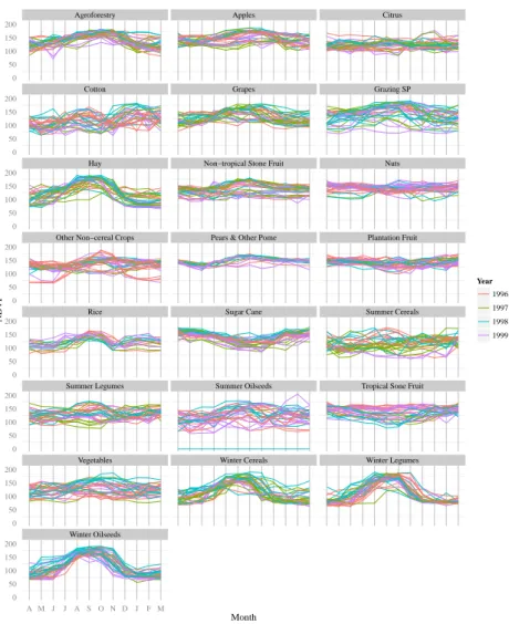
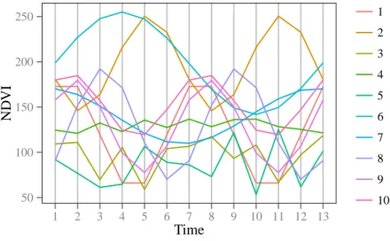
Maps were produced using a time series of 13 composite cloud-corrected NDVI images prepared
by the Environmental Resources Information Network (ERIN) from the AVHRR NDVI archive
covering the reference period. An image was created for each 28 day period in the year to 31
March (ignoring 31 March and 29 February); for each pixel, a spline was used to create an
NDVI value for each day and the value for each output image was the average of the daily
values for the period represented.
2.3.1.4 Control Site Data
Control sites were selected from a database of ground control points compiled over the period
1997 to 1999 for the production of the 1996–97 SPREAD map. The control site data were
collected by state and territory agencies (both government and private) using a mixture of field
work and analysis of aerial photos and satellite imagery (Stewart et al., 2001). Control sites for
a given commodity were sought in areas where that commodity was abundant according to the
1996–97 agricultural census. This database contains around 2871 suitable control sites, each
of which has location, LU and year attributes specifying the location of the site and the LU
occurring at the site in the year of observation. Observations were made for the years ending
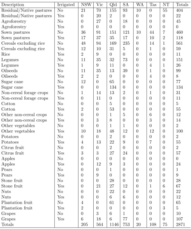
31 March 1997, 1998 and 1999 at each control site. Table 2.1 shows the total number of control
sites for each LU in each state (i.e. over all years). All control sites from all years were used
in mapping each LU in every SLA. We recognise that it is less than ideal to use training data
from different time periods to the one under consideration, or from locations as geographically
distant from the pixel under consideration as occurs with this limited database, but this was
Description Irrigated NSW Vic Qld SA WA Tas NT Totals
Residual/Native pastures No 21 70 155 93 10 0 55 404
Residual/Native pastures Yes 0 20 2 0 0 0 0 22
Agroforestry No 0 27 0 18 0 0 0 45
Agroforestry Yes 0 0 0 0 0 0 0 0
Sown pastures No 36 91 151 121 10 44 7 460
Sown pastures Yes 17 37 35 17 0 10 2 118
Cereals excluding rice No 48 94 169 235 0 14 1 561
Cereals excluding rice Yes 12 10 31 5 0 1 0 59
Rice Yes 2 9 0 0 0 0 0 11
Legumes No 11 35 32 73 0 0 0 151
Legumes Yes 1 9 11 0 0 4 1 26
Oilseeds No 11 35 13 39 0 1 0 99
Oilseeds Yes 2 2 0 0 0 4 0 8
Sugar cane No 12 0 65 0 0 0 0 77
Sugar cane Yes 0 0 134 0 0 0 0 134
Non-cereal forage crops No 1 14 13 2 0 1 0 31
Non-cereal forage crops Yes 0 11 0 0 0 0 0 11
Cotton No 0 0 5 0 0 0 0 5
Cotton Yes 2 0 53 0 0 0 0 55
Other non-cereal crops No 0 0 1 5 0 6 0 12
Other non-cereal crops Yes 0 3 8 0 0 3 0 14
Other vegetables No 0 0 1 1 0 0 0 2
Other vegetables Yes 10 18 48 12 0 12 0 100
Potatoes No 0 0 2 0 0 0 0 2
Potatoes Yes 4 13 22 9 0 7 0 55
Citrus fruit No 0 0 2 0 0 0 0 2
Citrus fruit Yes 3 3 27 24 0 0 0 57
Apples No 0 0 0 0 0 0 0 0
Apples Yes 0 12 9 3 0 0 0 24
Pears No 0 0 1 0 0 0 0 1
Pears Yes 0 9 0 0 0 0 0 9
Stone fruit No 0 0 28 0 0 0 0 28
Stone fruit Yes 0 21 27 12 0 1 6 67
Nuts No 0 0 22 0 0 0 0 22
Nuts Yes 0 0 6 6 0 0 0 12
Plantation fruit No 4 0 61 0 0 0 0 65
Plantation fruit Yes 2 0 0 0 0 0 3 5
Grapes No 0 3 6 1 0 0 0 10
Grapes Yes 6 18 6 77 0 0 0 107
Totals 205 564 1146 753 20 108 75 2871
2.3.1.5 Irrigation and Horticulture constraints
The data used for the irrigation constraint was based on an irrigation boundaries dataset
pub-lished by the National Land and Water Resources Audit (NLWRA) (National Land and Water
Resources Audit, 1999) and some additional Victorian irrigation areas. The horticulture
con-straints were based on various land cover datasets (Bureau of Rural Sciences, 1999, 2005). These
were converted to rasters of the same topology as the NDVI data. See Bureau of Rural Sciences
(2010a) for full details.
2.3.2 Running SPREAD II
The constant α from (2.2.2) was set to 70 percent for the irrigation constraint where there was sufficient area reported in the AgStats to achieve this. This was based on the observation
that 70 percent of the control sites with irrigated LU fell inside the irrigation mask. For the
horticulture mask α was set to 90 percent, where there was sufficient area reported in the AgStats to achieve this, based on the judgement that the horticulture mask is a reasonably
accurate representation of horticulture regions.
LUs for which the area prescribed in the AgStats was very small, or for which we had no control
sites, were removed and the areas of the remaining LUs were scaled up to retain the same total
area of agricultural LU according to the AgStats within the region.
The first stage of the SPREAD II algorithm was to allocate an initial LU to each pixel in the
SLA being analysed. This allocation was done by setting the LU for m pixels to k, where Pm
n=1an ≈µk, where an is the area of pixel n and µk is the area of LU k according to the AgStats. Note that any allocation of LUs to the pixels will suffice, but this method was chosen
so the algorithm starts close to the expectation of the ‘constraint’ distributions, [A|Θ]. We note
that the burn-in period for the algorithm could potentially be reduced further by allocating the
initial LU of each pixel based on [Cn=cn|Yn] (which can be calculated from [Yn|Cn =cn] in the obvious way assuming [Yn] is constant) and assigning LUs to the pixels as described above.
All pixels n ∈ {1, . . . , N} were then checked to ensure that [Yn|Cn = cn] > 0, where cn is the LU initially allocated to pixeln, and if it was not, the LU for the pixel was swapped with that of another such that both had non-zero probability for their allocated LU. In some rare
cases, a pixel had zero probability for all LUs. In this case, [Yn|Cn=k] was set to 1/K for all k∈ {1, . . . , K}.
Once the initial allocation was done, SPREAD II was run for a burn-in period of 2,000 iterations,
then a further 10,000 iterations from which the posterior probabilities of each LU for each pixel
were estimated using (2.7). Analysis of the outputs suggests that the burn-in of 2,000 iterations
is more than sufficient for the MCMC to ‘forget’ its initial state, and that a run length of 10,000
ismuch more than sufficient to get good estimates of the probability; good estimates could be
achieved with run lengths of around 1,000 in most cases. An analysis of the burn-in period is
presented in Section 2.4.1.4.
The variances contained in Θ were chosen to allow ‘room to move’ in the algorithm, rather
than realistic estimates of the variances of the AgStats estimates. This is partially justified in
used in the constraints should be based on the variances of the AgStats estimates.
2.3.3 Software
A range of software was used in constructing these versions of the NLUMs. Workstation
ARC/INFO software, Version 9.1 under SunOS was used for all Geographic Information
Sys-tems (GIS) operations, including:
• construction of the non-agricultural LU mask,
• construction of the irrigation and horticulture masks,
• scaling the AgStats to accord with the area of agricultural land identified in each region,
• extracting NDVI profiles for the control sites and the agricultural pixels and exporting them to a format that can be read by the SPREAD II software, and
• importing the SPREAD II outputs from ASCII Comma Separated Values (CSV) files
back into ESRI grid format.
The statistical package R (R Core Team, 2015) was used to do most of the preparation of the
data before running SPREAD II. This included:
• loading and preprocessing the AgStats data,
• calculating [Yn|Cn] by comparing the NDVI profiles of the control sites with those of the
target pixels,
• setting up the parameters of (2.2.2), and
• serialising the outputs of SPREAD II for post-processing using ARC/INFO.
SPREAD II itself was written in C++ and compiled as a shared library called from R. A small
PERL script was used to coordinate the running of the various scripts and programs over all
regions.
2.3.4 Results
SPREAD and SPREAD II were run across the entire continent of Australia. In this section we
present examples of the output of SPREAD II and quantitative and qualitative comparisons of
the NLUMs produced using SPREAD, SPREAD II, and the CLUM data.
2.3.4.1 Quantitative Comparison to the Catchment Scale Land Use Map of
Australia (CLUM)
While the CLUM has its limitations, it was the only source of ground truth data available. It is
was developed from the CLUM data. The preparation of the figures shown in this section was
done by Robert Smart of ABARES. Many of the details contained in the following description
are also due to Robert and correspondence with Australian Collaborative Land Use Mapping
Program (ACLUMP) members.
The NLUMs were overlaid on CLUM data with the same currency and the percentage of pixels
with matching LUs calculated. Two methods of matching were used:
1. pixels were awarded a match if both the NLUM and CLUM data had identical LU codes,
and
2. pixels were awarded a match if the NLUM and CLUM LU codes matched under one or
more of a set of rules that compensate for known limitations affecting the comparability
of these data. The rules used and the reason for applying them are given in tables 2.2
and 2.3, which were prepared by Robert Smart when preparing the validation data.
We refer to these two matching methods asexact andrelaxed hereafter.
The main limitations alluded to in the second matching method are:
• In the construction of the NLUMs for years up to and including 2001–02, it is assumed
that no grazing occurs in forested areas where the crown cover exceeds 50 percent. This
assumption leads to some misclassification of grazing (of natural vegetation and of
min-imally modified pastures) as conserved (mainly remnant native vegetation). Figure 2.2
illustrates this; much land is shown in the national scale maps as conserved that should
be shown asgrazing natural vegetation according to the catchment scale map.
• Distinguishing native and modified pasture has always been a problem for LU mapping. The AgStats data that we have used for the construction of NLUMs, from the 1992–93
agricultural census data up to and including the 2001–02 agricultural survey data, give
areas for sown pastures and native pastures, but always with a large shortfall. We have
assumed this is due to under-reporting of native pasture. Comparison of the NLUMs based
on these AgStats data with CLUM data suggests that the sown pasture areas reported in
the AgStats data do not account for all of the modified pasture. Some of what we have
mapped as native pasture in the NLUMs is really modified pasture, albeit pasture that
is only minimally modified, such as mosaics of native and exotic pastures. This is also
illustrated in Figure 2.2.
• The NLUMs and CLUM cannot be expected to show a high level of agreement with
respect to irrigation status as this is not well mapped in the CLUM, where it is generally
inferred from the presence of irrigation infrastructure.
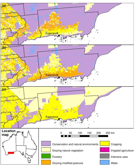
We chose CLUM data with currency 1996–97 covering a collection of land parcels in south-east
Victoria, and CLUM with currency 2000–01 covering a collection of land parcels in central
New South Wales (NSW) for comparison with NLUM data of the same currency. These two
collections of land parcels and are shown in Figure 2.1.
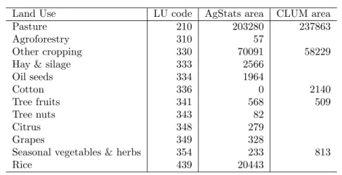
The areas of each LU are provided in Table 2.4. Non-agricultural LUs make up a small
(a) Central NSW test region (b) South-east Vic test region
(b) (a)
Lake Cargelligo Hillston
Dubbo Narromine
Bairnsdale
Morwell
0 20 40 60 80 100 km
0 20 40 60 80 100 km
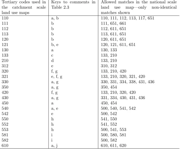
Tertiary codes used in the catchment scale land use maps
Keys to comments in Table 2.3
Allowed matches in the national scale land use map—only non-identical matches shown
110 a, b 110, 111, 112, 113, 117, 651
111 b 111, 651, 661
112 b 112, 611, 651
113 b 113, 611, 651
120 b 120, 611, 651
121 b, e 120, 121, 611, 651
130 a 130, 133
133 c 133, 210
210 d 133, 210
312 e 310, 312
320 f, g 133, 210, 420
321 e, f, g 133, 210, 320, 321, 420
330 a, g 330, 331, 334, 338, 431, 436
350 a, g 350, 454
420 f, g 133, 210, 320, 420
430 a, g 331, 334, 430, 431, 436
450 a 450, 454
540 a, e 500, 540, 541, 542
542 e 500, 542
550 h 541, 550
552 h 541, 552
553 h 500, 541, 553
581 i 500, 580, 581
582 i 500, 582
610 a, j 610, 611, 620
Tab. 2.2: Concordance between ALUM codes mapped in SPREAD II and accepted matches in the CLUM used for validation.
regions. In the south-east Victoria test regions, the agricultural land is almost entirely used
for grazing whereas in the central NSW test regions cropping and horticulture are almost as
prevalent asgrazing.
Comparisons were based on pixel counts rather than actual areas since the geographic extent of
each region is small and consequently the area of each pixel within each region is approximately
constant across the region. CLUM polygons were converted to a raster format with the same
coordinate system, cell size and cell alignment as the NLUM data. The LU assigned to each
CLUM pixel was that which occupied the largest proportion of the area covered by the pixel.
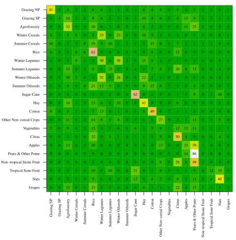
The percentage of pixels that matched based on the two criteria described above are given
in Table 2.5. The differences between SPREAD and SPREAD II appear to be minor, with
SPREAD doing slightly better in the case of exact matches and SPREAD II doing slightly
better in the relaxed matches.
2.3.4.2 Qualitative Comparisons in Selected Regions
The following comparisons present two regions where there are large differences between SPREAD,
SPREAD II and the CLUM.