A robust model structure selection method for small sample size and multiple datasets problems

This is a repository copy of A robust model structure selection method for small sample

size and multiple datasets problems.

White Rose Research Online URL for this paper:

http://eprints.whiterose.ac.uk/130275/

Version: Accepted Version

Article:

Gu, Y. and Wei, H.L. orcid.org/0000-0002-4704-7346 (2018) A robust model structure

selection method for small sample size and multiple datasets problems. Information

Sciences, 451-52. pp. 195-209. ISSN 0020-0255

https://doi.org/10.1016/j.ins.2018.04.007

[email protected] https://eprints.whiterose.ac.uk/

Reuse

This article is distributed under the terms of the Creative Commons Attribution-NonCommercial-NoDerivs (CC BY-NC-ND) licence. This licence only allows you to download this work and share it with others as long as you credit the authors, but you can’t change the article in any way or use it commercially. More

information and the full terms of the licence here: https://creativecommons.org/licenses/

Takedown

If you consider content in White Rose Research Online to be in breach of UK law, please notify us by

Final accepted version of the manuscript of the paper: Information Sciences, Volumes 451–452, July 2018, Pages 195-209

A Robust Model Structure Selection Method for Small Sample Size and Multiple

Datasets Problems

Yuanlin Gu, Hua-Liang Wei*

(Corresponding author:[email protected])

Department of Automatic Control and Systems Engineering, University of Sheffield, Sheffield, United Kingdom

Abstract: In model identification, the existence of uncertainty normally generates negative impact on the accuracy and

performance of the identified models, especially when the size of data used is rather small. With a small data set, least squares estimates are biased, the resulting models may not be reliable for further analysis and future use. This study introduces a novel robust model structure selection method for model identification. The proposed method can successfully reduce the model structure uncertainty and therefore improve the model performances. Case studies on simulation data and real data are presented to illustrate how the proposed metric works for robust model identification.

Keyword: nonlinear systems; systems identification; model uncertainty; model structure detection

1. Introduction

The procedure of model identification includes several steps including data collection and processing, selection of model representation, model structure detection and selection, model parameter estimation, and model validity test [25]. A wide variety of model types have been developed for nonlinear input-output system identification, modelling and control, for example, nonlinear autoregressive with exogenous inputs (NARMAX) model [15], neural networks [13,16,20,26], Bayesian network [19], fuzzy model [11,27,36,37,39], wavelet models [5,8,31,38] and so on. Among these, the NARMAX model is one of the most commonly used model types for many real-world applications including ecological systems [22], environmental systems [3], space weather [1,10,34], medicine [4], societal [18] and neurophysiological [21] sciences, etc.

Broadly speaking, data based modelling approaches can be categorized into two groups: parametric and nonparametric. Nonparametric methods are those that do not make strong assumptions about the form of the mapping functions (that map the model "input" variables to the model "output" variables). Most existing artificial neural networks are nonparametric approaches. In [24] it is stated that "Nonparametric methods are good when you have a lot of data and no prior knowledge, and when you don’t want to worry too much about choosing just the right features” (p.757). One of the advantages of neural networks is that in general they can achieve relatively higher performances in dealing with complicated data modelling problems defined in high dimensional space. However, the model structure of most neural networks is very complicated and cannot be simply written down. In addition, neural networks models often involve a large number of variables and take a long time for training. General neural networks models cannot provide a transparent model structure, where the significance of individual variables and the role of their interactions are invisible. Moreover, the implementation of some nonparametric approaches for example Bayesian networks normally would need a huge number of samples. In comparison with neural networks models, parametric NARX models use a nonlinear polynomial structure and often only need a small number of effective model terms to describe the system. It can be achieved by selecting a number of most important model terms by an orthogonal forward regression (OFR) algorithm [14,33], so that it generally only requires a relatively small number of input and output data points [6,30]. In many applications (e.g. [3],[4]), where the main objective of the modelling tasks is not only to predict future behavior, but also reveal and understand which model variables are most important and how the candidate variables interactively affect the system behavior, parametric models are usually become a first choice.

the following challenging question. Given a small set of experimental data of a system, how to build a model that best represents the underlying system dynamics hidden in the data? Most data modelling approaches can generate good models that best fit the data themselves, but the models may not be able to represent well the inherent dynamics of the original system because of different kinds of uncertainties. For small data modelling problems, the difficulty of finding reliable models is often exacerbated due to the small sample size of data. It is observed that for a small data modelling problem, small changes in a few or even a single sample can cause a large effect on model estimation. Thus, another question that arises is: how to reduce the model uncertainty (i.e. increase the model reliability) for small size data modelling problems?

It is not straightforward, if not impossible, to induce a robust model from a small sample size data, no matter what kind of system identification or data modelling algorithm are employed. In additional to noise and the size of samples, other types of factors can also lead to model uncertainty. For example, a data based modelling approach may just simply assumes a specific model type to represent the data but the specified model structure is completely different from the true system model; some driven variables may be immeasurable or ignored. All this is embedded in the aphorism “all models are wrong, but some are useful” [9]. In fact, for all system identification problems, model type selection and structure detection is usually an instrumentally important task. For the same data based modelling problem, different types of models often have different properties and performance, with different interpretation of the data. Even for the same model type, different algorithms could lead to different final model representations. The reason is simple: when the true model is unknown, all the identified models could be wrong because of uncertainty and the incompleteness of information. Effectively dealing with uncertainty (model structure, parameter, prediction, etc.) has become an important topic in many research fields, for example, soil changes [23], carbon and water fluxes at the tree scale [17]. In all scientific research, it nearly always needs to consider uncertainty, from various perspective such as, sources of uncertainty, techniques of quantifying uncertainty, decision making under strong uncertainty conditions, etc.

With the above observations, this study aims to develop a new approach to find a robust model structure to reduce uncertainty in model identification especially when sample size is small. Based on a data resampling approach, combined with an orthogonal forward regression (OFR) algorithm [14,33], a robust model structure selection (RMSS) method is designed to reduce model uncertainty and improve model performance. This is especially useful for the following two scenarios of data based modelling problem: i) modelling from multiple small sample size datasets (e.g. many datasets for a same system but generated under different experimental conditions; ii) modelling for a non-stationary system where although the key system dynamics can be represented using a single model structure, different model parameters are needed to adaptively reflect the change of system behaviors at different times.

In summary, the main contribution of the work lies in the new robust common model structure detection method for solving two challenging problems frequently encountered in practical system identification and data-driven modelling, namely, (a) reliable model identification from small sample data, and (b) robust common model determination from several or many experimental datasets.

The reminder of this paper is organized as follows. In Section 2, the classic nonlinear autoregressive moving average with exogenous inputs (NARMAX) model and orthogonal forward regression (OFR) algorithm are briefly reviewed. In Section 3, the proposed robust model structure selection (RMSS) method is introduced. Section 4 presents case studies of both simulation data and real data. The study is summarized in Section 5.

2. Overview of NARMAX model and OFR algorithm

This study focuses on linear-in-the-parameters representation including NARMAX model. The OFR algorithm is used to detect the significant model terms and establish parsimonious model structures.

2.1 NARMAX model

The nonlinear autoregressive moving average with exogenous inputs (NARMAX) model [15] was developed for black-box system identification where the true model structure is assumed to be unknown. The general NARMAX model structure is:

where and are systems output and input signals; is a noise sequence with zero-mean and finite variance. and are the maximum lags for the system output, input and noise. is some nonlinear function. Many of the traditional linear and nonlinear model type, for example, AR, ARM and NARX model can be treated as special cases of NARMAX model. There are several advantages of NARX and NARMAX model: first, the model structure can be determined in a stepwise way by selecting the significant model terms by an orthogonal forward regression (OFR) algorithm; second, the identification procedure is not time consuming and easy to implement; third, the polynomial form of the model provides a transparent and parsimonious representation of the system which is easy to understand and use. These advantages can be realized using an OFR method, which can effectively and efficiently select model terms, from a huge number of candidate model terms.

2.2 Term Selection using OFR algorithm

The classic OFR algorithm, firstly introduced in [14], was originally developed as a subset selection method for nonlinear modelling problems where the nonlinearity is unknown in advance and the desirable model terms cannot be specified. The OFR method was proposed in solving such ‘black-box’ system identification problems. The basic idea behind this method is to use an error reduction ratio (ERR) [14] index, to measure the significance of candidate model terms and generate a rank according to the contribution made by each of the model terms to explaining the variation of the response variable. At each step, one model term can be selected from the candidate sets according to their ERR ranking. After each term is selected, it is removed from the bases and the bases are then transformed to new orthogonalized bases for the next terms selection procedure. The OFR algorithm can be described as follows:

2.2.1 Problem Statement

A polynomial NARX model can be written as the following linear-in-the-parameters form:

(2)

where are the model terms generated from the regressor vector

, are the unknown parameters and M is the number of candidate model terms.

Let be the output vector of N sampled observations and be the

vector formed by the m-th model term . A dictionary of all the candidate model terms can be written as . And let be a subset of model terms, from the full set , where

. Thus, the term selection problem for the (2) is to find a subset so that can be well explained:

(3)

2.2.2 Model Term Selection

The classic OFR method uses a simple and effective ERR index, to measure the contribution of each model term in exampling the system. For the full dictionary , the ERR index of each candidate model term can be calculated by:

(4)

where . The first selected model term can then be identified as:

(5)

Then the 1st significant model term of the subset can be selected as , and the 1st associated orthogonal variable can be defined as . After removal from , the dictionary is then reduced to a sub-dictionary , consisting of model candidates. At step , the bases are first transformed into new group of orthogonalised

base with orthogonlization transformation.

where are orthogonal vectors, ) are the basis of unselected model terms

of subset and are the new orthogonalised bases. The rest of the model terms can then

be identified step by step using the ERR index of orthogonalised subsets :

(7)

(8)

2.2.3 Model size determination

The selection procedure can be terminated when specific conditions are met. The number of model terms to be included in the final model can be determined by several model selection criteria, for example, the Generalised Cross-Validation (GCV) [8], a modified Generalised Cross-Validation Criteria based on Mean-Square-Error (MSE) [22], a modified ESR (Error Signal Ratio) index [28] and the adjustable prediction error sum of squares (APRESS) [6]. In this study, the APRESS is used to determine the number of model terms. It is given as:

(9)

where is the number of observations, is the number of selected model terms, is a small positive number and is the mean square error. The optimal number of model terms is often chosen as:

(10)

The above procedure is referred to as forward regression with orthogonal least squares (FROLS) or simply orthogonal forward regression (OFR) algorithm [7,14].

3. Robust model structure selection method

Following the discussions in the previous section, the OFR method is used to select a small number of significant terms to establish a best model structure. For many real modelling tasks, there are several commonly seen situations where the OFR algorithm cannot be directly used to generate best models, for example: i). the data are usually recorded from a series of experiments under different experimental conditions, or the system itself is non-stationary and needs to be observed for a long-time scale. In these scenarios, the model structure might be varying with time and/or with the change of external environmental conditions. ii). The true model structure of the system is unknown and cannot be well represented by any of the candidate model terms in the dictionary. Thus, it is impossible to find a perfect model structure and there will always be uncertainty of model structure. iii). the data is corrupted with strong noises which makes the OFR estimation biased. The bias could be extremely obvious when data size is small, since a small change of a single term can bring a huge difference on the estimated model. Under these conditions, the OFR method may fail to find a best model structure that can well represent the system. Therefore, the RMSS method is needed for capturing and reducing the model uncertainty and thus improving the overall model predictive performance.

In the following, a novel RMSS method is proposed. The basic idea of the new method is first illustrate using a simple example, and the procedure of the method is then presented.

3.1 Basic idea

Table 1

Variables of two datasets

x1 x2 x3 y

1 1 0 1

dataset 1 0 1 1 2

1 1 1 5

1 0 0 4

0 1 0 2

dataset 2 1 1 1 1

0 0 0 3

1 0 0 1

Assuming that one and only one variable (among x1, x2, and x3) is used to fit the two datasets, then which one can give a

minimum OMAE value? This can be done by calculating the individual MAE values one by one. For example, the

individual mean absolute error of the variable x for dataset 1 can be calculated as:

₍₁₁₎

MAEs for x2 and x3 can be calculated in a similar way for datasets 1. Similar calculations can be performed to dataset

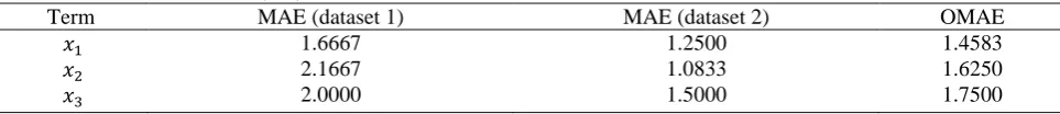
2. There is a total number of 6 individual MAEs. The OMAEs can be calculated, as shown in Table 2. As the OMAE value of x1 is smaller than the other two, x1 should be the best choice for fitting the two datasets. Note that once the first

model term is determined, a second model term can be chosen to join the first one, and then a third one, and on. The detailed descriptions of the general procedure of the RMSS method is given in next section.

Table 2

MAE and OMAE values of x1, x2, and x3

Term MAE (dataset 1) MAE (dataset 2) OMAE

1.6667 1.2500 1.4583

2.1667 1.0833 1.6250

2.0000 1.5000 1.7500

3.2 Robust model structure selection method

The RMSS method can be summarized into several steps:

3.2.1 Resampling process (for small size data)

Assume that the original data can be described by a matrix as follows:

(12)

(13)

where the associated candidate basis vectors become and is the number of data points in each sub-dataset.

Remark 1: For small size data, the original dataset is resampled by removing one of the data points each time until all the

data points have been picked out once (leaving one sample out), so that and . Thus, the uncertainty brought by removing or adding a single data point can be reduced by finding a single common model for the K sub-datasets. The resampling process is used for the situations when the data size is small and the effect of a single data point can be significant for determining the final model structure and model parameters.

3.2.2 The OMAEs of model terms for K sub-datasets

To find a robust model structure that best fits all the sub-datasets, an MAE matrix is calculated using the data from all the sub-datasets. In the first step search, the MAE matrix is defined as:

(14)

where is the individual MAE value when the m-th candidate model term is

used to approximate output in the k-th sub-dataset. It is calculated as:

(15)

where is the parameter. Then, the OMAE associated with the m-th candidate model term which is used to represent all the sub-datasets is defined as: (16)

Remark 2: In addition to the OMAE, there are several other metrics for measuring the overall predicted error of each model term, for example: (17)

(18)

(19)

(20)

where y and are the observed and predicted system outputs and is the number of data points. As will be illustrated later (e.g. Table 12 in Section IV-B) that y y (MAE) is a better choice. It was argued in some studies that MAE is a better metric for model evaluation [12].

(21)

Then the 1st significant model terms can be selected as . After removal of the basis from the k-th sub-dataset

the dictionaries of all the sub-datasets are then reduced and consists of model candidates. Similar to that in the conventional OFR algorithm, at step , the dictionaries consist of candidate

model terms. The bases are all transformed into a new group of orthogonalized bases. The orthogonal transformation can be implemented using (6) for each single sub-dataset. The MAE matrix at step can be calculated using the new group of bases, and the MAE matrix is:

(22)

The OMAEs of all the candidate terms can then be calculated and the s-th robust model term can be selected to be , with:

(23)

Repeating the recursive process, a number of model terms can be selected to form a linear-in-parameters robust model structure. Similar to OFR algorithm, the selection procedure can be terminated when specific conditions are met.

Assume that a total of model terms are selected, and for the -th sub-dataset let the output be represented by the selected model terms as:

(24)

Following [14,15], the model parameters can be calculated through an iterative procedure. According to the orthogonalization procedure [14,15], here we define unity upper triangular matrices first:

(25)

where .

From the orthogonalization procedure, the elements of can be calculated as:

(26)

(27)

The estimates of K groups of parameter vector can then be calculated from the triangular equations . The final model parameter estimation is chosen to be the average of the parameter estimates, with:

(28)

Detailed derivation and explanation for the mechanism of the above calculations (25)-(28) can be found in [14] and [15].

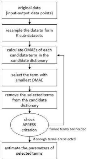
Remark 3: The proposed RMSS method can be summarized into several steps: 1). calculate the OMAE of each candidate

transformed the rest of bases to form new orthogonalized bases; 4) repeat the first 3 steps until a specific model selection criterion is met. 5). parameter estimation. The whole procedure can be described by a diagram as shown in Fig. 1.

Remark 4: Note that different from traditional L2-norm based algorithms, e.g. the orthogonal projection pursuit (OPP)

algorithm [28] that can be proven to converge, the proof of the convergence of the proposed RMSS method is not straightforward. In this study, the focus is on choosing a set of most powerful model terms from a given pool consisting of a large number of candidate model terms, through an iterative manner, one term at each search step, until a model with an appropriate model terms that gives satisfactory fit to the data is obtained. Instead of strictly prove the convergence of the proposed method, we demonstrate the overall performance of the new method through numerical case studies which are presented in the next section.

Fig. 1. Robust model structure selection (RMSS) method

4. Case studies

Two simulation examples are presented to test the efficiency of the RMSS method and to show under which conditions the proposed method can improve the model performance. The first example aims to test if the proposed method can pick out the correct model terms when data are noise free. The second example investigates the performance of the proposed method for modelling problems with different levels of uncertainty (noise). Finally, a case study on Kp index forecast is carried out to demonstrate the power of the new method solving a real-world problem. For the convenience of comparative analysis, the model identified by OFR method will be referred as ‘regular model’ and the model identified by RMSS method will be referred as ‘robust model’.

4.1 Example 1- noise free data modelling

It is known that most existing model structure selection methods are able to provide sufficiently reliable model, when data are clean (i.e. not corrupted with noise). In the following it will show that both the RMSS method and classic OFR method can generate perfect model structure from noise free data. Consider a nonlinear system:

y t y t u t t (29)

where the input u t was assumed to be uniformly distributed on . A total number of 100 input-output data points were generated. The first 70 points were used for model estimation and the remaining 30 points were used for performance test. The following candidate variable vector was used for model construction:

The initial full model was chosen to be a polynomial form with nonlinear degree of l . Firstly, the OFR method was applied to find the significant model terms according to the ERR ranking. The APRESS values suggest that a model of 5 terms can be a good choice. Not surprisingly, all the model terms are correctly selected and the parameters are estimated correctly. The selected terms and the associated ERR values are shown in Table 3. The RMSS method was also applied to the same train data, to select significant terms according to their OMAEs relating to a total number of 70 sub-datasets generated through the resampling process. As a result, the RMSS method selected exactly the same model terms as the OFR method. The associated OMAEs are shown in Table 4.

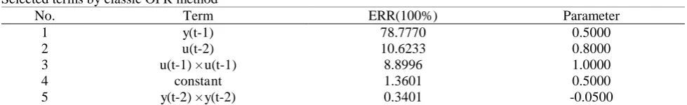
Table 3

Selected terms by classic OFR method

No. Term ERR(100%) Parameter

1 y(t-1) 78.7770 0.5000

2 u(t-2) 10.6233 0.8000

3 u(t-1) × u(t-1) 8.8996 1.0000

4 constant 1.3601 0.5000

5 y(t-2) × y(t-2) 0.3401 -0.0500

Table 4

Selected terms by RMSS method

No. Term OMAE Parameter

1 y(t-1) 0.5639 0.5000

2 u(t-2) 0.3831 0.8000

3 u(t-1) × u(t-1) 0.1610 1.0000

4 constant 0.0652 0.5000

5 y(t-2) × y(t-2) 0.0000 -0.0500

Fig. 2. SERR and OMAE versus the number of iteration of term selection

Note that the OFR and RMSS methods employ two different indicators (i.e., the ERR index and OMAEs to measure the contribution of each model term to explaining the variance of response variable. During the process of OFR, the SERR (sum of ERR values) is increasing to the maximum value of 100%, which indicates that 100% of the variance of response variable can be explained by the selected terms. For the RMSS method, the OMAE is decreasing to 0, which means that there is no error in the identified model. The variation of SERR and OMAE of the OFR and RMSS are displayed in Fig. 2. It can be easily seen that the model with 5 terms is perfect and can describe 100% of the variance of the response variable. The variation of the correlation coefficient and prediction efficiency, with the inclusion of model terms, one by one, is shown in Fig. 3.

4.2 Example 2- data with additive white noise Now consider a nonlinear system:

(31)

where the input was assumed to be uniformly distributed on and is a white noise with zero mean and finite variation. With five different levels of signal to noise ratio, namely, noise-free and SNR = 50, 15, 10, 0 dB, respectively, the system was simulated five times. For each SNR case, a total number of 100 input-output data points were generated. The first 70 points were used for model estimation and the remaining 30 points were used for performance test. The initial full model was chosen to be a polynomial form with maximum time lags of and nonlinear degree

of . Note that the model term was not included in the specific library of candidate model terms. As a consequence, it is impossible to identify a ‘true’ model structure that perfectly represents every single component of the system. However, it is possible to use both the OFR and the RMSS method to find model that can well represent the simulated data. In what follows, it presents analysis and discussions on whether the RMSS methods can find satisfactory models with good predictive performance, under different level of noise.

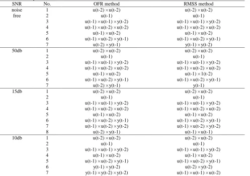
Table 5

Selected terms by OFR and RMSS method

SNR No. OFR method RMSS method

noise free

1 u(t-2) × u(t-2) u(t-2) × u(t-2)

2 u(t-1) u(t-1)

3 u(t-1) × u(t-1) × y(t-2) u(t-1) × u(t-1) × y(t-2)

4 u(t-1) × u(t-2) × u(t-2) u(t-1) × u(t-2) × u(t-2)

5 u(t-1) × u(t-2) u(t-1) × u(t-2)

6 u(t-1) × u(t-2) × y(t-1) u(t-1) × u(t-2) × y(t-1)

7 u(t-2) × y(t-1) y(t-1) × y(t-2)

50db 1 u(t-2) × u(t-2) u(t-2) × u(t-2)

2 u(t-1) u(t-1)

3 u(t-1) × u(t-1) × y(t-2) u(t-1) × u(t-1) × y(t-2)

4 u(t-1) × u(t-2) × u(t-2) u(t-1) × u(t-2) × u(t-2)

5 u(t-1) × u(t-2) u(t-1) × 1(t-2)

6 u(t-1) × u(t-2) × y(t-1) u(t-1) × u(t-2) × y(t-1)

7 u(t-2) × y(t-1) y(t-1)

15db 1 u(t-2) × u(t-2) u(t-2) × u(t-2)

2 u(t-1) u(t-1)

3 u(t-1) × u(t-1) × y(t-2) u(t-1) × u(t-1) × y(t-2)

4 u(t-1) × u(t-2) × u(t-2) u(t-1) × u(t-2) × u(t-2)

5 u(t-1) × u(t-2) u(t-1) × u(t-2)

6 u(t-1) × u(t-2) × y(t-1) u(t-1) × u(t-2) × y(t-1)

7 u(t-1) × u(t-2) × y(t-2) u(t-1) × u(t-2) × y(t-2)

8 u(t-2) × y(t-1) u(t-1) × u(t-1)

10db 1 u(t-2) × u(t-2) u(t-2) × u(t-2)

2 u(t-1) u(t-1)

3 u(t-1) × u(t-1) × y(t-2) u(t-1) × u(t-1) × y(t-2)

4 u(t-1) × u(t-2) u(t-1) × u(t-2)

5 u(t-1) × u(t-2) × y(t-1) u(t-1) × u(t-2) × y(t-1)

6 y(t-1) × y(t-2) u(t-2) × y(t-2)

8 u(t-1) × u(t-2) × u(t-2) y(t-2) × y(t-2) × y(t-2)

9 u(t-1) × u(t-1) × u(t-2) u(t-1) × u(t-2) × y(t-2)

0db 1 u(t-2) × u(t-2) u(t-2) × u(t-2)

2 u(t-1) u(t-1)

3 u(t-2) × u(t-2) × y(t-2) u(t-2) × u(t-2) × y(t-2)

4 u(t-1) × u(t-1) × y(t-1) y(t-1) × y(t-1)

5 u(t-1) × u(t-2) u(t-2) × y(t-2)

6 u(t-1) × u(t-1) u(t-2) × u(t-2) × u(t-2)

7 y(t-1) × y(t-1) u(t-2) × y(t-2) × y(t-2)

8 y(t-1) × y(t-2) y(t-1) × y(t-1) × y(t-1)

9 y(t-1) × y(t-1) × y(t-1) u(t-1) × u(t-1) × y(t-2)

Both the OFR and RMSS methods were applied to the simulated data with different levels of noises (noise-free, SNR = 50, 15, 10, 0 dB). The model complexity was determined by the APRESS metric. The selected model terms by the two methods are shown in Tables 5. It can be observed that for most cases, the two methods select the same model terms for the first few steps. This is reasonable because these terms are the most significant terms and make major contribution to explaining the variance of system output and leaving one sample out (this scheme is used in RMSS method but not in OFR) does not affect the order of the selected terms. However, the two methods start to select different model terms after a few steps. These model terms give smaller contributions to explaining the variance in output signal, and a small change of single sample might affect result of selection of these terms. In other words, the less significant model terms are more sensitive to the effect of noise.

As mentioned earlier, the classic OFR method uses ERR index as measure to select model terms; the measure is defined as how much (in percentage) of the variance in the response signal can be explained by a newly included model term. The RMSS method uses OMAE instead, which is a measure of the averaged prediction error in relation to a great number (say ) of models estimated from sub-datasets generated from the original data through a resampling process. Therefore, the resulting robust model should provide better overall predictive performances than the regular model. The performance statistics of the regular and robust models are given in Table 6. The results show that with the decrease in SNR values, the performance of the models identified by both the OFR method and the robust method decreases, due to the increase of uncertainty. It should be stressed that even for the noise-free case, both of the two methods fail to detect the true model

structure, because the model component is actually not in the pre-defined library of candidate model terms.

Table 6

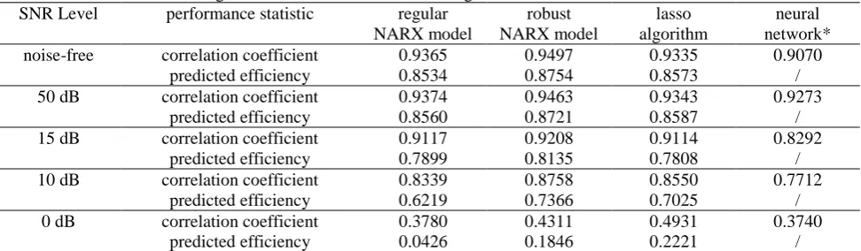
Performance statistics of the regular model, robust model, lasso algorithm and neutral networks under different noises

SNR Level performance statistic regular

NARX model robust NARX model lasso algorithm neural network*

noise-free correlation coefficient 0.9365 0.9497 0.9335 0.9070

predicted efficiency 0.8534 0.8754 0.8573 /

50 dB correlation coefficient 0.9374 0.9463 0.9343 0.9273

predicted efficiency 0.8560 0.8721 0.8587 /

15 dB correlation coefficient 0.9117 0.9208 0.9114 0.8292

predicted efficiency 0.7899 0.8135 0.7808 /

10 dB correlation coefficient 0.8339 0.8758 0.8550 0.7712

predicted efficiency 0.6219 0.7366 0.7025 /

0 dB correlation coefficient 0.3780 0.4311 0.4931 0.3740

predicted efficiency 0.0426 0.1846 0.2221 /

* The number of layers is 10 and the training algorithm is Levenberg-Marquardt. The algorithm was run for 10 times and the averaged correlation coefficient is recorded.

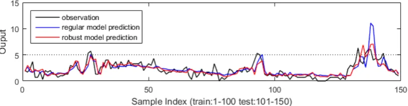
Comparing the performance statistics of the regular and robust NARX models given, it is clear that the robust models outperform the regular models in all the cases. In addition, the improvement of the robust models is significant when SNR is quite low say at 10 dB and 0 dB. Fig. 4-6 show the model prediction of the regular and robust models for the three cases: noise-free and SNR=15dB and 0dB, respectively. As can be seen from the figures, the differences of predicted and observed output become more significant with the increase of noise level. It can be noted in Fig. 6 that there are some extremely large values in predicted output from the regular model, and the robust model is more conservative in prediction, where the amplitudes of the predicted values are in general smaller than that of the classical model but closer to the true values.

unnecessary model terms to zero. The lasso method can be easily adapted to many application scenarios where the desired response signal is assumed to be of a sparse representation of a set of independent signals (predictors).However, lasso could fail to produce stable subset selection results when the predictors are highly correlated. The performances of the two methods are evaluated based on the models with the same number of model terms. From the results in Table 6, the robust NARX model outperforms the lasso method in most of the cases (noise-free, SNR=50, 15, 10 dB). This is because the orthogonal forward regression (OFR) algorithm used in RMSS can effectively solve sever correlation and ill-conditioning problems [30,33]. Regarding all the five cases, the performances of the neural network models are lower than those of the other two methods. This might be because that the size of the data is very small, and that the power of neural networks is cannot be fully exploited for this small size data modelling problem. More importantly, the proposed RMSS method has the following superiorities: i). the procedure is easy to implement and not time-consuming; ii). the identified model clearly indicates the information of the most important model terms; iii). the identified model provides a transparent and parsimonious linear-in-the-parameters representation, which can be easily generalized to new data. It is worth mentioning that in this example, all the robust models were built using only 70 data points, which is quite small. This means the proposed RMSS method may promise an effective data driven modelling approach for nonlinear systems, especially for small size data with strong uncertainty. Overall, these results show the clear advantage of the proposed RMSS method in nonlinear model identification.

In addition, for the case of SNR=15dB, three extra robust models are obtained based on the other three different measures defined in (21)-(23), respectively. The performance statistics of all the four models are given in Table 7 and it turns out that the robust model selected by OMAE over performs the other three models.

Table 7

Comparison of the performances of robust models identified based on different measures Measures

Correlation Coefficient 0.9208 0.9202 0.8667 0.8667

Predicted Efficiency 0.8135 0.8059 0.7018 0.7018

Fig. 4. One-step-ahead (OSA) predictions of robust model and regular model (noise free)

Fig. 6. One-step-ahead (OSA) predictions of robust model and regular model (SNR is 10dB)

4.3 Example 3- Kp index Forecasting

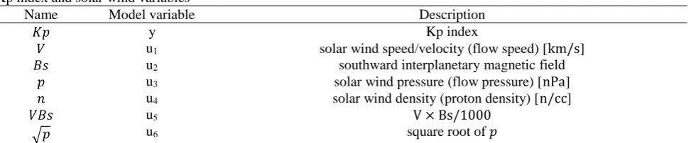
Magnetic disturbance can affect many equipment and systems on or nearby earth, for example, navigation systems, communication systems, satellites, and power grid, etc. They can be paralyzed and unreliable during these severe magnetic situations. In order to understand and forecast the geomagnetic activity, the Kp (planetarische Kennziffer) index was first introduced by Bartels in 1949 [2]. The value of Kp index ranges from 0 (very quiet) to 9 (very disturbed) in 28 discrete steps, resulting values of 0, 0+, 1-, 1, 1+,2-, 2, 2+, …, 9 [35]. The Kp index has been recorded and updated since last century and become an important dataset to study space weather. The correlation between Kp index and solar wind parameters has been discovered by many researches. Normally, the solar wind variables are treated as the model inputs and Kp index is treated as the model output. A full description of the solar wind variables and derived variables is summarized in Table 8.

Table 8

Kp index and solar wind variables

Name Model variable Description

y Kp index

u1 solar wind speed/velocity (flow speed) [km s]

u2 southward interplanetary magnetic field

u3 solar wind pressure (flow pressure) [nPa]

u4 solar wind density (proton density) [n cc]

u5 V Bs

u6 square root of

The Kp index was sampled every 3 hours and the solar wind variables were sampled every 1 hour. It should be noted that this study aims to build the models using robust method to predict Kp index 3 hours ahead. Therefore, the unit of time lags of both input and output is 3 hours. For example, is the Kp index recorded 6 hours before and ) is the solar wind speed recorded 3 hours before A total number of 150 input-output data points of the 2011 are selected for the case study. The maximum time lags are chosen as and the nonlinear degree is 2. The first 100 samples are used for training and the remaining 50 samples are used for testing. The model is selected using only input lag variables, without using autoregressive variables. The first 4 model terms selected by OFR method and RMSS method are shown in the following table 9 and table 10.

Table 9

Selected terms by OFR method for Kp model

No Term ERR(100%) Parameter

1 u6(t-1) 79.6551 7.7057e+00

2 u2(t-1) × u2(t-1) 5.3507 4.0605e+02

3 u1(t-1) 2.5907 2.3494e+00

4 u2(t-2) 0.3058 7.4787e+00

Table 10

Selected terms by RMSS method For Kp model

No Term OMAEs Parameter

1 u6(t-1) 0.85592 6.4929e+00

3 u1(t-1) × u6(t-2) 0.68803 2.0516e+01

4 u5(t-1) 0.65544 -8.2486e+04

The performance statistics of the two models are given in Table 11 and Fig. 7 presents comparisons between the model outputs and the associated measurements. Clearly, the overall performance of the robust model is better than the regular model and that produced by the lasso algorithm. The performance of the neural network model is slightly better than the robust NARX model. However, it is worth noting that the robust NARX model uses a much less number of model terms to provide a transparent and parsimonious representation, which is easy to interpret and use. Although the correlation between the measurements and the corresponding prediction of the neural network model is higher, the model itself is very complicated and difficult to write down. In contrast, the RMSS method and NARX model provide a transparent and parsimonious representation, which is simple where all the interactive relation among variables is clear. In general, the RMSS method achieves a good trade-off between model complexity and model performance. Overall, the robust NARX model can be a good choice for Kp index predictions.

Table 11

Performance statistics of the regular model and robust model on Kp forecast

Performance Statistics regular model robust model lasso neural networks*

Correlation Coefficient 0.7132 0.8056 0.6109 0.8368

Predicted Efficiency 0.2927 0.6304 0.3202 /

Normalized Root Mean Square Error 0.2449 0.1750 0.3506 /

* The number of layers is 10 and the training algorithm is Levenberg-Marquardt. The algorithm was run for 10 times and the averaged correlation coefficient is recorded.

Fig. 7. One-step-ahead (OSA) predictions of robust model and regular model for Kp index

5. Conclusion

This article focuses on improving model identification methods from small size data. When the size of data is small or data is corrupted with noises, there is large uncertainty of model structure and parameter. These conditions can bring a negative effect on the model structure selection process of the classic OFR method. In this study, the RMSS method is proposed to enhance the classic OFR algorithm by selecting the robust significant model terms according to the OMAEs of resampled sub-datasets. The new method is tested on two simulation examples and a real data application. The results suggest that the new method can improve the prediction performance of modelling problems, especially when the data size is small and there are strong noises and unknown system components. The advantage of this robust model is that it can better capture the inherent dynamics of the whole dataset and thus can be well generalized to new data. Thus, the new method can be applied for small sample size and multiple datasets problems.

Acknowledgements

This work was supported in part by EU Horizon 2020 Research and Innovation Programme Action Framework under grant agreement 637302, the Engineering and Physical Sciences Research Council (EPSRC) under Grant EP/I011056/1 and Platform Grant EP/H00453X/1.

References

[1] M.A. Balikhin, R.J. Boynton, S.N. Walker, J.E. Borovsky, S.A. Billings, H.L. Wei, Using the NARMAX approach to model the evolution of energetic electrons fluxes at geostationary orbit, Geophys. Res. Lett. 38 (2011) 1–5. doi:10.1029/2011GL048980.

[2] J. Bartels, The standardized index, Ks, and the planetary index, Kp, IATME Bull. 126 (1949).

[3] G.R. Bigg, H.L. Wei, D.J. Wilton, Y. Zhao, S.A. Billings, E. Hanna, V. Kadirkamanathan, A century of variation in the dependence of Greenland iceberg calving on ice sheet surface mass balance and regional climate change, Proc. R. Soc. A Math. Phys. Eng. Sci. 470 (2014) 20130662–20130662. doi:10.1098/rspa.2013.0662.

[4] C.G. Billings, H.L. Wei, P. Thomas, S.J. Linnane, B.D.M. Hope-Gill, The prediction of in-flight hypoxaemia using non-linear equations, Respir. Med. 107 (2013) 841–847. doi:10.1016/j.rmed.2013.02.016.

[5] S.A. Billings, H.L. Wei, The wavelet-NARMAX representation: A hybrid model structure combining polynomial models with multiresolution wavelet decompositions, Int. J. Syst. Sci. 36 (2005) 137–152. doi:10.1080/00207720512331338120.

[6] S.A. Billings, H.L. Wei, An adaptive orthogonal search algorithm for model subset selection and non-linear system identification, Int. J. Control. 81 (2008) 714–724. doi:10.1080/00207170701216311.

[7] S.A. Billings, Nonlinear system identification: NARMAX methods in the time, frequency, and spatio-temporal domains, 2013.

[8] S.A. Billings, H.L. Wei, A new class of wavelet networks for nonlinear system identification., IEEE Trans. Neural Netw. 16 (2005) 862–874. doi:10.1109/TNN.2005.849842.

[9] G.E.P. Box, N.R. Draper, Empirical Model-Building and Response Surfaces, 1987. doi:10.1037/028110.

[10] R.J. Boynton, M.A. Balikhin, S.A. Billings, H.L. Wei, N. Ganushkina, Using the NARMAX OLS-ERR algorithm to obtain the most influential coupling functions that affect the evolution of the magnetosphere, J. Geophys. Res. Sp. Phys. 116 (2011) 1–8. doi:10.1029/2010JA015505.

[11] H. Bustince, E. Barrenechea, M. Pagola, J. Fernandez, Z. Xu, B. Bedregal, J. Montero, H. Hagras, F. Herrera, B. De Baets, A historical account of types of fuzzy sets and their relationships, IEEE Trans. Fuzzy Syst. 24 (2016) 179–194. doi:10.1109/TFUZZ.2015.2451692.

[12] T. Chai, R.R. Draxler, Root mean square error (RMSE) or mean absolute error (MAE)? -Arguments against avoiding RMSE in the literature, Geosci. Model Dev. 7 (2014) 1247–1250. doi:10.5194/gmd-7-1247-2014.

[13] S. Chen, S.A. Billings, Neural networks for nonlinear dynamic system modelling and identification, Int. J. Control. 56 (1992) 319–346. doi:10.1080/00207179208934317.

[14] S. Chen, S.A. Billings, W. Luo, Orthogonal least squares methods and their application to non-linear system identification, Int. J. Control. 50 (1989) 1873–1896. doi:10.1080/00207178908953472.

[15] S. Chen, S.A. Billings, Representations of non-linear systems: The NARMAX model, Int. J. Control. 49 (1989) 1013– 1032. doi:10.1080/00207178908559683.

[16] S. Chen, S.A. Billings, P.M. Grant, Non-linear system identification using neural networks, Int. J. Control. 51 (1990) 1191–1214. doi:10.1080/00207179008934126.

[17] M. Christina, Y. Nouvellon, J.P. Laclau, J.L. Stape, O.. Campoe, G. le Maire, Sensitivity and uncertainty analysis of the carbon and water fluxes at the tree scale in Eucalyptus plantations using a metamodeling approach 1, Can. J. For. Res. 46 (2016) 297–309. doi:10.1139/cjfr-2015-0173.

[18] Y. Gu, H.L. Wei, Analysis of the relationship between lifestyle and life satisfaction using transparent and nonlinear parametric models, 2016 22nd Int. Conf. Autom. Comput. (2016) 54–59. doi:10.1109/IConAC.2016.7604894.

[19] H. Guo, X. Liu, Z. Sun, Multivariate time series prediction using a hybridization of VARMA models and Bayesian networks, J. Appl. Stat. 43 (2016) 2897–2909. doi:10.1080/02664763.2016.1155111.

[20] S. Haykin, Neural networks-A comprehensive foundation, New York IEEE Press. Herrmann, M., Bauer, H.-U., Der, R. psychology (1994) pp107-116. doi:10.1017/S0269888998214044.

[21] Y. Li, H.L. Wei, S.A. Billings, P.G. Sarrigiannis, Identification of nonlinear time-varying systems using an online sliding-window and common model structure selection (CMSS) approach with applications to EEG, Int. J. Syst. Sci. 47 (2016) 2671–2681. doi:10.1080/00207721.2015.1014448.

heterogeneous responses of fish community size structure using novel combined statistical techniques, Glob. Chang. Biol. 22 (2016) 1755–1768. doi:10.1111/gcb.13190.

[23] N.J. Robinson, K.K. Benke, S. Norng, Identification and interpretation of sources of uncertainty in soils change in a global systems-based modelling process, Soil Res. 53 (2015) 592. doi:10.1071/SR14239.

[24] S. Russell, P. Norvig, Artificial Intelligence: A Modern Approach, 3rd Ed, Prentice Hall, Upper Saddle River, NJ. (2010).

[25] J.R.A. Solares, H.L. Wei, S.A. Billings, A novel logistic-NARX model as a classifier for dynamic binary classification, Neural Comput. Appl. (2017) 1–15. doi:10.1007/s00521-017-2976-x.

[26] H. Wang, H.R. Karimi, P.X. Liu, H. Yang, Adaptive neural control of nonlinear systems with unknown control directions and input dead-zone, IEEE Trans. Syst. Man, Cybern. Syst. (2017). doi:10.1109/TSMC.2017.2709813. [27] H. Wang, W. Liu, P.X. Liu, H.K. Lam, Adaptive fuzzy decentralized control for a class of interconnected nonlinear system with unmodeled dynamics and dead zones, Neurocomputing. 214 (2016) 972–980. doi:10.1016/j.neucom.2016.07.019.

[28] H.L. Wei, S. A. Billings, Generalized cellular neural networks (GCNNs) constructed using particle swarm optimization for spatio-temporal evolutionary pattern identification, Int. J. Bifurc. Chaos. 18 (2008) 3611. doi:10.1142/S0218127408022585.

[29] H.L. Wei, S.A. Billings, Improved model identification for non-linear systems using a random subsampling and multifold modelling (RSMM) approach, Int. J. Control. 82 (2009) 27–42. doi:10.1080/00207170801955420.

[30] H.L. Wei, S.A. Billings, Model structure selection using an integrated foward orthogonal search algorithm assisted by square correlation and mutual information, Int. J. Model. Identif. Control. 3 (2008) 341–356. doi:10.1504/IJMIC.2008.020543.

[31] H.L. Wei, S.A. Billings, A unified wavelet-based modelling framework for non-linear system identification: The WANARX model structure, Int. J. Control. 77 (2004) 351–366. doi:10.1080/0020717042000197622.

[32] H.L. Wei, S.A. Billings, Improved parameter estimates for non-linear dynamical models using a bootstrap method, Int. J. Control. 82 (2009) 1991–2001. doi:10.1080/00207170902854118.

[33] H.L. Wei, S.A. Billings, J. Liu, Term and variable selection for non-linear system identification, Int. J. Control. 77 (2004) 86–110. doi:10.1080/00207170310001639640.

[34] H.L. Wei, S.A. Billings, A. Surjalal Sharma, S. Wing, R.J. Boynton, S.N. Walker, Forecasting relativistic electron flux using dynamic multiple regression models, Ann. Geophys. 29 (2011) 415–420. doi:10.5194/angeo-29-415-2011. [35] S. Wing, J.R. Johnson, J. Jen, C.I. Meng, D.G. Sibeck, K. Bechtold, J. Freeman, K. Costello, M. Balikhin, K. Takahashi, Kp forecast models, J. Geophys. Res. Sp. Phys. 110 (2005). doi:10.1029/2004JA010500.

[36] S. Yin, P. Shi, H. Yang, Adaptive fuzzy control of strict-feedback nonlinear time-delay systems with unmodeled dynamics, IEEE Trans. Cybern. 46 (2016) 1926–1938. doi:10.1109/TCYB.2015.2457894.

[37] L. A. Zadeh, Fuzzy sets, Inf. Control. 8 (1965) 338–353. doi:10.1016/S0019-9958(65)90241-X.

[38] Q. Zhang, A., Benveniste, Wavelet networks, IEEE Transactions on Neural Networks 3 (1992) 889–898.