A solution decomposition for a singularly perturbed fourth-order problem

A solution decomposition for a singularly perturbed fourth-order

problem

Sebastian Franz, Katharina H¨

ohne, Marcus Waurick

November 18, 2015

Abstract

We consider a singularly perturbed fourth-order problem with third-order terms on the unit square. With a formal power series approach, we decompose the solution into solutions of reduced (third-order) problems and various layer parts. The existence of unique solutions for the problem itself and for the reduced third-order problems is also addressed.

Key words: asymptotic expansion, singular perturbations, fourth-order problem, boundary layers

AMS subject classifications: 35B25, 35C20, 35G15

1

Introduction

In the present paper we are concerned with the singularly perturbed problem

Lψ:=ε∆2ψ+ (b_{· ∇)∆ψ−c∆ψ=f in Ω = (0,1)}2_,

ψ= 0 on Γ =∂Ω, ∂nψ= 0 on Γ,

(1.1)

where b_{= (b1, b2) withb1, b2 >0 andc >0 are given, and the perturbation parameterεis supposed to} be very small with 0< ε≪1.

The problem (1.1) arises from different physical models. In particular, the equations (1.1) can be formally derived from the Oseen equations, that is, from the streamfunction-vorticity formulation of the Oseen equations. In this context the parameter ε is the reciprocal of the Reynolds number. If the Reynolds number gets very large, the flow is said to be turbulent. Although the Oseen equations are usually considered as a model for the moderate Reynolds-number regime, we are interested in the high-Reynolds number case and see the Oseen equations as linearisation of the non-linear Navier-Stokes equations.

Apart from the motivation in fluid dynamics fourth-order problems are frequently studied, when mod-elling plate-bending problems. In contrast to our problem, this kind of problems is well understood and numerical analysis can be found, see [2,3,5,7,8], just to name a few. The main difference, however, is that the equations treated in the references cited do not contain third-order terms. Thus, the corresponding reduced problem is elliptic which simplifies the asymptotic analysis.

Our method of choice for finding a proper solution decomposition into an interior part (arising from solutions of third-order problems) and layer parts is the method of asymptotic expansions. This approach can, for instance, be found in [4, 10, 11, 13], where it is applied to second-order problems. Roughly rephrasing the rationale of asymptotic expansions, we consider a reduced problem, where formally ε is set to 0 and certain boundary conditions are neglected, to construct solution parts that are independent ofε. The misfit of certain boundary conditions is then corrected by boundary layer terms. As an ansatz for the boundary layer terms, we choose functions that exponentially decay away from the boundary.

More precisely, with the exponentially decaying functions

E1(x) = e−b1

x

ε and E

2(y) = e−b2

y ε,

our final result reads as follows: Assuming appropriate conditions on the right-hand sidef, the solution

ψ of (1.1) admits a decomposition

ψ(x, y) =S(x, y) +εH(x, y)E1(x) +εI(x, y)E2(y) +ε2J(x, y)E1(x)E2(y),

where the functions S, H, I and J are bounded independently of ε. Similar decompositions do also hold for the first derivatives. In the one-dimensional case solution decompositions already exist in the literature, see, for instance, [17]. The decompositions given there contain so-called “weak layers”: A property shared by the decomposition derived in this exposition. Here, we call a functionweak layer, if it is exponentially decaying away from the boundary, itsL∞_{-norm vanishes forε→0 but theL}∞_-norm

of its derivative does not.

The structure of this paper is as follows. The existence of unique solutions to (1.1) is shown and some of the solution’s properties are given in Section 2. In this section, we also put (1.1) into an (abstract) functional analytic perspective. The methods are based on (more or less standard) perturbation theory for linear operators and a crucial regularity result established in [2]. In order to establish a connection between the data of (1.1) and its solution we present a stability estimate in Section 3, which relies on results of [14]. Finally, Section 4 contains the derivation of the decomposition mentioned above.

Notation

Throughout this article, the domain Ω will be the unit square (0,1)2_{. Unless it is clear from the context,}

we will denote by k · kX the norm of the Banach space X. Moreover, we will frequently neglect the

reference to the underlying domain D of certain Lebesgue or Sobolev spaces, that is, we will write, for instance, k · kL2 instead ofk · k_L2_(D).

2

Existence and uniqueness of solutions

This section is devoted to the proof of existence and uniqueness of solutions of (1.1), for anyf ∈L2_(Ω).

We approach the problem from an abstract point of view in Subsection 2.1. The findings are then applied to (1.1) in Subsection 2.2.

2.1

Perturbation theorems for operators in Hilbert spaces

In this subsection we shall elaborate on some elements of perturbation theory of linear operators in Hilbert spaces. Large parts can be found in the standard reference [9, Chapter III]. As some of the well-known results focus on selfadjoint/symmetric operators, some of the theorems might not be directly applicable. Hence, we provide full proofs of the respective results, though the general techniques employed are not new. The final aim of this section is to establish a proof of Theorem 2.6. For stating and eventually proving the theorem, we need the following notion of relative boundedness.

Definition 2.1 Let H be a Hilbert space, A:D(A)⊆H →H,B:D(B)⊆H →H be linear operators.

B is called A-boundedwithA-boundκ≥0, ifD(B)⊇ D(A)and for allκ′_{> κ there existsC}

κ′ >0 such

that for all φ∈ D(A)the inequality

kBφk ≤κ′kAφk+Cκ′kφk

holds true. The operatorB is called infinitesimallyA-bounded, ifB isA-bounded with A-bound0.

For later use, for a linear operatorA: D(A)⊆H →H in a Hilbert space H, we denote the space D(A), the domain ofA, endowed with the graph scalar product ofA byDA. Recall that A is a closed

operator if and only ifDA is a Hilbert space.

Remark 2.2 Let, in this remark, Ω := (0,1)n_⊆Rn _{for somen∈N.}

(a) Let j ∈ {1, . . . , n}. Consider the operator ∂j: Hj1(Ω) ⊆ L2(Ω) → L2(Ω), f 7→ ∂jf, where

H1

j(Ω) := {f ∈ L2(Ω);∂jf ∈ L2(Ω)}. Then the operator ∂j is infinitesimally ∂j2 bounded. This is a

direct consequence of [9, p. 191].

(b) For any k, m ∈ N_{>0, k > m, and κ > 0 there exists Cκ > 0 such that for all φ ∈ H}k_{(Ω) the}

inequality

kφkHm≤C_κkφk_L2+κkφk_Hk (2.1)

holds true. In order to prove the claimed inequality (2.1), we proceed by induction: The casek≥2 and

m= 1 is a consequence of part (a) and of the Lipschitz continuity of the embeddingHk_֒→Hℓ_{for every}

k > m. Letκ >0 andk > m+ 1. Employing the induction hypothesis, we find Cκ>0 such that for all

φ∈Hm+1_(Ω)

kφkHm+1≤ kφk_L2+

n

X

j=1

k∂jφkHm

≤ kφkL2+

n

X

j=1

(Cκk∂jφkL2+κk∂_jφk_Hk−1).

By part (a) and the fact thatk≥2, for κ′ _{>0 there existsC}

κ′ >0 such that we may estimate further

kφkHm+1≤ kφk_L2_(Ω)+

n

X

j=1

CκCκ′kφk_L2+C_κκ′kφk_Hk_(Ω)+κk∂_jφk_Hk−1

≤(1 +nCκCκ′)kφk

L2+ (nC_κκ′+κ)kφk_Hk.

The latter inequality yields the proof of the inductive step.

(c) Let k, m ∈ N_{>0, k > m. Let A:D(A) ⊆ L}2_{(Ω) → L}2_{(Ω) be closed with D(A) ⊆ H}k_(Ω),

B:Hm_{(Ω) →L}2_{(Ω) linear and bounded. Then B considered as an operator inL}2_{(Ω) is infinitesimally}

A-bounded. Indeed, the canonical embeddingι:DA֒→Hk(Ω) is well-defined. Moreover, as the mapping

DA ֒→L2(Ω) is continuous, the operator ι is closed. Using the closedness of A, we infer thatDA is a

Hilbert space. Hence,ιis continuous by the closed graph theorem. In particular, there existsC >0 such that for allφ∈ D(A) we have1

kφkHk≤Ckφk_DA ≤CkAφk_L2+Ckφk_L2.

Next, take φ∈ D(A). Letκ >0 and let Cκ>0 as in (2.1). Then, denoting bykBkHm_→L2 the operator

norm ofB as an operator mapping from Hm _toL2_{, we compute forφ∈ D(A)}

kBφkL2 ≤ kBk_Hm_→L2kφk_Hm

≤ kBkHm_→L2C_κkφk_L2+kBk_Hm_→L2κkφk_Hk

≤ kBkHm_→L2C_κkφk_L2+kBk_Hm_→L2κ(CkAφk_L2+Ckφk_L2)

= (kBkHm_→L2C_κ+kBk_Hm_→L2κC)kφk_L2+κkBk_Hm_→L2CkAφk_L2,

which implies the assertion.

Lemma 2.3 Let H be a Hilbert space, A: D(A) ⊆H →H, B:D(B) ⊆ H → H be linear operators.

Assume that A is closed and that B is A-bounded with A-bound κ < 1. Then A+B is closed with

D(A+B) =D(A)

Proof

Note that, by the A-boundedness ofB, D(B)⊇ D(A). Hence, the natural domain of A+B coincides with the one of A. Thus, only the closedness needs to be shown. For this, let C > 0 be such that kBxk ≤Ckxk+κ′_{kAxk for someκ}′_{<1. Then, we compute}

kAxk ≤ k(A+B)xk+kBxk ≤ k(A+B)xk+Ckxk+κ′kAxk (x∈ D(A))

Hence,kxk+ (1−κ′_{)kAxk ≤ k(A+B)xk+ (C+ 1)kxk (x∈ D(A)). On the other hand, we realize}

k(A+B)xk+kxk ≤(1 +κ)kAxk+ (C+ 1)kxk (x∈ D(A)).

Therefore, the normsk · k+kA· kandk · k+k(A+B)· kare equivalent, proving the assertion.

We recall that ifA is a selfadjoint operator in a Hilbert spaceH, that is, we haveA=A∗_{, then the}

operator Ais necessarily closed and densely defined.

For properly computing the adjoint of the sumA+B, we need a condition onB∗_:

Lemma 2.4 LetH be Hilbert space,A:D(A)⊆H →H,B:D(A)⊆H →H linear operators. Assume

that Ais selfadjoint, D(B)⊇ D(A)and thatB∗ _{isA-bounded with A-bound<1. Then}

(A+B)∗=A+B∗

1_{In the applications to be discussed later on, the inequality will be guaranteed right away so that we do not really need}

We need the following prerequisit.

Lemma 2.5 Let H be a Hilbert space, A: D(A) ⊆H →H, B: D(B) ⊆ H → H be linear operators.

Assume that A is selfadjoint and that B is A-bounded with A-bound <1. Then there exists z ∈ ρ(A)

such that

kB(A−z)−1k<1. Proof

By hypothesis, there exists 0≤κ <1 andCκ≥0 such that for allx∈ D(A), we have

kBxk ≤κkAxk+Cκkxk.

Next, as for anyr∈R_{\ {0}by the self-adjointness ofA, we infer}

k(A−ir)−1k ≤ 1 |r|.

Thus, we get for allx∈H andr∈R_{\ {0},}

kB(A−ir)−1xk2≤ κkA(A−ir)−1xk+Cκkxk

2

≤ κ2kA(A−ir)−1xk2_{+ 2κC}

κkA(A−ir)−1xkk(A−ir)−1xk+Cκ2k(A−ir)−1xk2

≤κ2kxk2+ 2κCκ 1

|r|kxk

2_+C2

κ

1

r2kxk 2

≤

κ2+ 2κCκ

1 |r| +C

2

κ

1

r2

kxk2_,

where we used the selfadjointness ofAto estimatekA(A−ir)−1_{k ≤1.}

Next, we prove Lemma 2.4. The proof of which has been kindly communicated to the authors by Rainer Picard.

Proof (Lemma 2.4)

By Lemma 2.5, we findz∈ρ(A) such thatkB∗_(A−z)−1_{k<1. Next, we observe that}

(A−z∗₎−1_{B= (B}∗_(A−z)−1₎∗_.

In fact, the equality being clear on the domain of B, so the equality is plain since B is densely defined and the operator on the right-hand side is continuous. In particular, we infer thatk(A+µ)−1_{Bk<1 for}

µ:=−z∗_.

For proving the claim of the lemma, we takex∈ D((A+B+µ)∗_{). Then for ally ∈ D(A+B+µ),}

the equality

h(A+B+µ)y, xi=hy,(A+B+µ)∗xi

holds true. For y∈ D(A+B+µ) puttinguy:= (1 + (A+µ)−1B)y, we compute

(A+B+µ)y= (A+µ)y+By= (A+µ)(1 + (A+µ)−1_{B)y= (A+µ)u}

y.

Hence,

h(A+µ)uy, xi=h(1 + (A+µ)−1B)

−1

uy,(A+B+µ)∗xi,

or, expressed differently, for allw∈ R((1 + (A+µ)−1_B)|

D(A)) we infer

h(A+µ)w, xi=h(1 + (A+µ)−1_B)−1_w,(A+B+µ)∗_xi.

Next, observe thatR((1+(A+µ)−1_B)|

D(A)) is dense inH, sinceD(A) is dense inHand (1+(A+µ)−1B)

is an isomorphism. Therefore, the continuous extension of the functional

R((1 + (A+µ)−1B)|D(A))∋w7→ h(1 + (A+µ)−1B)

−1

w,(A+B+µ)∗xi

defines an element ofD(A∗_{). Hence,x∈ D((A+µ)}∗_{) =D(A) and}

(A+µ)∗x= (1 + (B∗((A+µ)∗)−1))−1(A+B+µ)∗xi,

or

(A+B)∗_x+µ∗_{x= (A+B+µ)}∗_{x= (1 + (B}∗_((A+µ)∗₎−1_))(A+µ)∗_{x= (A+µ}∗_+B∗_)x,

We finally come to the main result of this subsection. We recall that an operatorA:D(A)⊆H →H

is called non-negative, if for allφ∈ D(A), we have thathAφ, φi ≥0.

Theorem 2.6 Let H be a Hilbert space, A: D(A)⊆H → H be selfadjoint and non-negative. Assume

that B:D(B)⊆H →H is linear,B andB∗ _{beingA-bounded with A-bound κ <1. Assume there exists}

c >0 such that for allφ∈ D(A) we have

ℜhBφ, φiH≥chφ, φiH andℜhB∗φ, φiH≥chφ, φiH.

Then the operator A+B is continuously invertible withk(A+B)−1_{k ≤1/c.}

Proof

By Lemma 2.3, the operatorA+B is closed withD(A+B) =D(A). The same is true for the operator

A+B∗_{. Next, forφ∈ D(A) using the non-negativity ofA, we estimate}

ℜh(A+B)φ, φi ≥ ℜhBφ, φi ≥chφ, φiH. (2.2)

The latter inequality (2.2) implies that A+B is invertible on its range R(A+B)⊆H with Lipschitz constant 1/c. We emphasize that the closedness ofA+Btogether with (2.2) also implies thatR(A+B)⊆ H is closed. From Lemma 2.4, we deduce that (A+B)∗_=A+B∗_{. Hence, from}

ℜh(A+B)∗φ, φi=ℜh(A+B∗)φ, φi ≥ ℜhB∗φ, φi ≥chφ, φiH (φ∈ D((A+B)∗) =D(A))

it follows that (A+B)∗ _{is one-to-one. The decomposition H =N((A+B)}∗_{)⊕ R(A+B) thus yields}

that A+B is onto, asR(A+B) is closed.

2.2

The fourth-order problem

In this section, we provide the well-posedness theorem for the fourth-order problem under consideration, see (1.1). For this, we start out with the problem with bandc formally set to zero. We introduce some operators from vector calculus in order to formulate the fourth-order problem in a proper functional analytic framework.

Definition 2.7 Let Ω⊆Rn _{open. Then define}

gradc:Cc∞(Ω)⊆L2(Ω) →L2(Ω), φ7→(∂jφ)_{j∈{1,...,n}}

divc:Cc∞(Ω)n⊆L2(Ω)n→L2(Ω), (φj)j∈{1,...,n}7→

n

X

j=1

∂jφj

∆c:Cc∞(Ω)⊆L2(Ω) →L2(Ω), φ7→ n

X

j=1

∂j2φ.

Moreover, we set

grad :=−div∗c, div :=−grad∗c, ∆ := ∆∗c

as well as

˚

grad := gradc, div := div˚ c, ∆ := ∆˚ c.

In order to relate the operators just introduced to the equation under consideration, we investigate the domain of ˚∆ a bit further:

Theorem 2.8 LetΩ = (0,1)2_{. Then∆ = ˚˚ div ˚grad, in other words,φ∈ D(˚∆)satisfies both homogeneous}

Dirichlet and Neumann boundary conditions.

Proof

From ∆|C∞

c (Ω)= ˚div ˚grad|C ∞

c (Ω) it follows that ˚∆ = ˚div ˚grad. Hence, it suffices to show that ˚div ˚grad is

closed. For this, let (un)n in D( ˚div ˚grad) withun→f and ˚div ˚gradun→g in L2(Ω) asn→ ∞for some

f, g∈L2_{(Ω). Observe that forn, m∈N, we have}

kgrad(˚ un−um)k2=−h(un−um),div ˚˚ grad(un−um)i →0 (n, m→ ∞).

Thus, (un)n is a Cauchy-sequence in D( ˚grad) endowed with the graph norm. Thus, f ∈ D( ˚grad) and

˚

gradf = lim

n→∞

˚

gradun, by the closedness of grad. Moreover, as both ( ˚˚ gradun)n and ( ˚div ˚gradun)n are

convergent inL2_(Ω)n_andL2_{(Ω), respectively, we infer, by the closedness of ˚div that ˚gradf ∈ D( ˚div) and}

˚

Remark 2.9 (On the domain of ˚div ˚grad) (a) The boundary of Ω = (0,1)2 _{is Lipschitz. Hence, by}

a standard regularity result, we have

D( ˚grad) =H01(Ω) ={u∈H1(Ω);u= 0 on∂Ω}.

Moreover,

D( ˚div) ={u_{∈ D(div);}u_·n_{= 0 on∂Ω},}

where u_·n_{is the normal component ofu. Hence, the domain of ˚div ˚grad can be characterised by}

D( ˚div ˚grad) ={u∈ D(div grad);u= 0, ∂nu= 0 on∂Ω},

where ∂nuis the normal derivative ofu.

(b) With the help of (a), the boundary conditions in equation (1.1) may be interpreted equivalently in two ways. The first way is that the boundary conditions may be understood in the sense of traces. Secondly, for a solutionψ∈L2_{(Ω) of (1.1), any summand should belong toL}2_{(Ω) and the equation (not}

including the boundary conditions) should hold in a distributional sense. The boundary conditions are realised as the additional condition of ψbelonging to the domain of ˚∆.

Remark 2.10 (On the regularity of D(˚∆)-functions) Note that Theorem 2.8 in particular implies that ˚∆⊆div ˚grad =: ∆D, where the indexDstands for homogeneous Dirichlet boundary conditions. So,

˚

∆ is a restriction of the Dirichlet Laplacian. It is known that, on convex domains, the Dirichlet Laplacian admits optimal regularity, that is, D(∆D) =H2(Ω)∩H01(Ω). So, D(˚∆) = H02(Ω) :={u∈ H2(Ω);u=

0, ∂nu= 0 on∂Ω}.

Remark 2.11 (a) It is a consequence of the Poincar´e inequality that the operator−˚∆ is strictly positive. Indeed, we have for allφ∈ D(˚∆) that

−h∆˚φ, φi=−hdiv ˚˚ gradφ, φi=hgrad˚ φ,grad˚ φi ≥c2Pkφk2L2

forcP >0 being the Poincar´e constant on the square Ω = (0,1)2.

(b) The inequality in (a) shows that ˚∆ is one-to-one and has closed range. It is standard (see, e.g., [19, Corollary 2.5]) that the range of ˚∆∗ _{= ∆ is closed itself. As ˚∆ is one-to-one, the operator ∆}

is onto. Moreover, by [19, Theorem 2.6], the operator|∆˚∆|=p∆˚∆ is continuously invertible inL2_(Ω).

Hence, so is|∆˚∆|2_{= ∆˚∆.}

Next, we cite a crucial result for our approach, which asserts that – similar to the Dirichlet Laplacian (cf. Remark 2.10) – the operator ∆˚∆ admits optimal regularity on Ω = (0,1)2_{, that is, D(∆˚∆) =}

H4_(Ω)∩H2 0(Ω).

Theorem 2.12 ([2, Theorem 2]) The operator

∆˚∆ :D(∆˚∆)⊆L2(Ω)→L2(Ω)

is continuously invertible and there existsd >0 such that for all φ∈ D(∆˚∆) we have the estimate

kφkH4_(Ω)≤dk∆˚∆φk_L2_(Ω).

Proof

The continuous invertibility has been established in Remark 2.11 (b). The regularity result is one of the

statements in [2, Theorem 2].

For the proof of the continuous invertibility of the operator

G:=ε∆˚∆ + (b· ∇)˚∆−c˚∆ (2.3)

in L2_{(Ω) forb∈R}2 _{andc >0, we will employ the abstract results found in the previous section.}

The next result shows thatε∆˚∆ is in fact the leading term in the operatorG. We briefly recall that any operator of the formA∗_{Ais selfadjoint and non-negative, whereAis a densely defined, closed linear}

Lemma 2.13 The operator

T:D(∆˚∆)⊆L2_(Ω)→L2_{(Ω), u7→((b· ∇)˚∆−c˚∆)u}

is infinitesimally ∆˚∆-bounded.

Proof

By Theorem 2.12, D(∆˚∆) =H4_(Ω)∩H2

0(Ω)⊆H4(Ω). Next, the operator

(b· ∇)∆−c∆ :H3_(Ω)→L2_(Ω)

is continuous. In addition, note that the operator ∆˚∆ = ˚∆∗_{˚∆ is selfadjoint, hence, closed. Thus, by}

Remark 2.2(c), considered in L2_{(Ω), the operator (b· ∇)∆−c∆ is infinitesimally ∆˚∆-bounded. We}

conclude with the observation that onD(∆˚∆) the operator T coincides with (b· ∇)∆−c∆. Lemma 2.14 Let T be given as in Lemma 2.13. Then the inclusionD(T)⊆ D(T∗_)holds.

Proof

We will use again Theorem 2.12, that is D(∆˚∆) =H4_(Ω)∩H2

0(Ω). So, for φ, ψ ∈H4(Ω)∩H02(Ω), we

compute for j∈ {1,2}

h∂j˚∆φ, ψi=h∂j∆φ, ψi

=h∆∂jφ, ψi

=h∂jφ,∆˚ψi

=h˚∂jφ,∆˚ψi

=−hφ, ∂j˚∆ψi,

where we denoted by ˚∂j the minimal closed restriction of the distributional derivative operator∂j with

respect to thej’th coordinate in L2_{(Ω) withC}∞

c (Ω) as a core. Moreover, we have

−h˚∆φ, ψi=hgrad˚ φ,grad˚ ψi=−hφ,∆˚ψi,

which establishes the assertion.

Remark 2.15 Note that in the proof of Lemma 2.14, we also showed that forφ∈ D(∆˚∆), we have

T∗φ=−(b· ∇)˚∆φ−c∆˚φ.

Thus, from this equality and Lemma 2.13 it follows thatT∗ _{is infinitesimally ∆˚∆-bounded, as well.}

Lemma 2.16 Let T be given as in Lemma 2.13. Then for all φ∈H4_(Ω)∩H2

0(Ω), the estimates

ℜhT φ, φi ≥cc2Phφ, φiandℜhT∗φ, φi ≥cc2Phφ, φi

hold true. Here cP >0 is the constant in Poincar´e’s inequality, see also Remark 2.11.

Proof

Both the asserted inequalities are shown in the same way. Hence, we stick to the first inequality only. We compute, using Remark 2.15, for φ∈H4_(Ω)∩H2

0(Ω):

2ℜhT φ, φi=ℜhT φ, φi+ℜ(hT φ, φi)∗ =ℜhT φ, φi+ℜhφ, T φi =ℜhT φ, φi+ℜhT∗φ, φi

=ℜh(b· ∇)˚∆φ−c∆˚φ, φi+ℜh−(b· ∇)˚∆φ−c∆˚φ, φi =−2ℜhc∆˚φ, φi

≥2cc2

Phφ, φi,

where we also used Remark 2.11(a).

Finally, we are in the position to prove the well-posedness result for the operatorG:

Theorem 2.17 The operatorGas given in (2.3)is continuously invertible with domainD(G) =H4_(Ω)∩

H2

0(Ω). Moreover, kG−1k ≤1/(cc2P), wherecP >0 is the Poincar´e constant given in Remark 2.11.

Proof

For the proof, we use Theorem 2.6 applied to A =ε∆˚∆ and T =B, where T is given in Lemma 2.13. We will now show that the assumptions of Theorem 2.6 are met. First of all note that the operator

ε∆˚∆ = ε∆˚∗_{˚∆ is selfadjoint and non-negative. Next, the operators T and T}∗ _{are infinitesimally ∆˚}

2.3

A third-order problem

We conclude Section 2 with a brief summary of the results of [20], which are relevant for our analysis to be carried out later on.

Definition 2.18 We call the problem

(b_{· ∇)∆ψ−c∆ψ=f inΩ,}

ψ= 0 onΓ, ∂nψ= 0 onΓ−,

(2.4)

whereΓ−:={x∈Γ :−b·n<0} is the inflow boundary, the reduced problemof (1.1).

Definition 2.19 A functionψfrom the classC1,h_{( ¯Ω)∩C}3_{(Ω)is a classical solutionof the problem (2.4)}

if it satisfies the equation and its boundary conditions. By C1,h_{(Ω), we denote the space of functions}

which are in C1_{(Ω) and whose derivatives satisfy the H¨older condition for 0< h <1.}

Proposition 2.20 Let f ∈C1,h_{( ¯Ω)andc≥0. Then the problem (2.4)has a classical solution which is}

unique.

Proof

For the proof, see [20, Theorems 1 & 2].

In [20], Zikirov shows the unique solvability for a more general problem, that is, for non-local boundary conditions. For our subproblems arising later, we also need solvability for such problems. To guarantee unique solvability, Zikirov states compatibility conditions (see [20, Problem 1]) for the boundary data that read in our case:

Proposition 2.21 The third-order problem

(b_{· ∇)∆ψ−c∆ψ=f inΩ,}

4ψ(0, y) =ϕ1(y), ψ(1, y) =ϕ2(y), ∂xψ(1, y) =ϕ3(y), 0≤y≤1,

ψ(x,0) =κ1(x), ψ(x,1) =κ2(x), ∂yψ(x,1) =κ3(x) 0≤x≤1,

where b_{= (b1, b2) withb1, b2>0 andc≥0 are constant, has a unique solution if the following}

compati-bility conditions are fulfilled:

ϕ1(0) =κ1(0), ϕ1(1) =κ2(0), κ1(1) =ϕ2(0), ϕ2(1) =κ2(1),

∂xκ1(1) =ϕ3(0), ∂yϕ1(1) =κ3(0), ∂xκ2(1) =ϕ3(1), ∂yϕ2(1) =κ3(1).

3

A stability estimate

Another important tool for the asymptotic analysis is a stability estimate. For the statement, we recall

Cα_{(I) for any interval I ⊆R, the space of α-H¨older continuous functions onI endowed with the usual}

norm. The special cases α = 0 and α = 1 yield the space of continuous functions and continuously differentiable functions, respectively. Similarly, we make use of fractional order Sobolev spacesHα_{(I) on}

bounded intervals,α∈R_{≥0, being the complex interpolation spaces of the respective Sobolev spaces with}

integer values. We recall from [18] the following essential properties of the H¨older spaces and fractional order Sobolev spaces.

Theorem 3.1 ([18, Sect 4.5.2 Rem 2, Sect 2.4.2 Rem 2(d), Sect 4.2.2 Thm]) Let I ⊆ R _{be a}

bounded closed interval. Then forα∈(0,1) there existd1, d2>0 such that

kfkCα_(I)≤d₁kfk1−α

C0_(I)kfk

α

C1_(I) and kgk_Hα_(I)≤d₂kgk1−α

H0_(I)kgk

α H1_(I)

for all f ∈C1_(I),g∈H1_(I).

Definition 3.2 Consider two functionsg1∈C1(∂Ω)∩H3/2(∂Ω)(more explicitlyg1∈C1(Γi)∩H3/2(Γi),

where Γi are the edges of the unit square) and g2∈C(∂Ω)∩H1/2(∂Ω). We say (g1, g2)are admissible

boundary values, if there exists a functionφ∈ D(∆2), such that

We now consider the following problem

ε∆2ψ+ (b_{· ∇)∆ψ−c∆ψ=f in Ω = (0,1)}2_,

ψ=g1 on Γ =∂Ω,

∂nψ=g2 on Γ,

(3.1)

where (g1, g2) are admissible boundary values andf ∈L2(Ω).

In the following, whenever appropriate, we stick to the custom of denoting byC >0 a generic constant independent ofε.

Theorem 3.3 Consider problem (3.1). The solution ψcan be estimated by

kψkL∞

(Ω)≤C ε−1 kfkL2_(Ω)+kg₁k_C1/2_(∂Ω)+kg₂k_L2_(∂Ω)

+kg1kC1_(∂Ω)+kg₂k_C(∂Ω)

.

Furthermore, we have

kψkH1_(Ω)≤Cε−1 kfk_L2_(Ω)+kg₁k_C1/2_(∂Ω)+kg₂k_L2_(∂Ω).

Before proving this theorem, we collect some intermediate results in two lemmas.

Lemma 3.4 Consider problem(3.1)with homogeneous boundary conditions, that is, assumeg1=g2= 0.

The solutionu∈H2

0(Ω)∩H4(Ω) can then be estimated by

kukH2_(Ω)≤Cε−1kfk_H−2_(Ω).

Proof

Foru∈H2

0(Ω)∩H4(Ω), using integration by parts and divb= 0, we get

ℜh(b_{· ∇)∆u, ui=−ℜhu,(}b_{· ∇)∆ui,}

which yields

ℜh(b_{· ∇)∆u, ui= 0.}

Thus, we get from the differential equation

ℜhf, uiL2 =ℜhLu, ui

=ℜh ε∆2u+ (b_{· ∇)∆u−c∆u, ui} =εk∆uk2_L2_(Ω)+ck∇uk2_L2_(Ω).

Hence,

εk∆uk2L2_(Ω)+ck∇uk2_L2_(Ω)≤ kfk_H−2_(Ω)kuk_H2_(Ω).

Using the equivalence of theH2_{-norm and u7→ k∆uk}

L2_(Ω) inH₀2 (cf. Remark 2.10), we get the desired

result.

Lemma 3.5 Let(g1, g2)be admissible boundary values. Letv∈H2(Ω)be the variational solution of the

problem

∆2_{v= 0 in Ω = (0,1)}2_,

v=g1 on Γ =∂Ω,

∂nv=g2 on Γ.

(3.2)

The triple(v, g1, g2)∈H1(Ω)×H1/2(∂Ω)×H−1/2(∂Ω)can also be understood as a generalised solution

of (3.2)in the sense of [12, Theorem 3.2.1]. Then,v fulfils the following estimate

kvkH1_(Ω)≤C kg₁k_H1/2_(∂Ω)+kg₂k_H−1/2_(∂Ω)

.

Proof

Letw∈H2

0(Ω) be the variational solution of the problem

∆2w= ∆v−v in Ω = (0,1)2, w= 0 on Γ =∂Ω, ∂nw= 0 on Γ.

(3.3)

It follows from [2, Theorem 2] that w∈H3_{(Ω) and}

kwkH3_(Ω)≤Ck∆v−vk_H−1_(Ω)≤Ckvk_H1_(Ω). (3.4)

Furthermore, we find a functionz∈H1_{(Ω) with z=g}

1 on∂Ω in the sense of traces and

kzkH1_(Ω)≤Ckg₁k_H1/2_(∂Ω), (3.5)

see [6, Corollary B.53]. With the help of Green’s formula, we get

0 = Z

Ω

(∆2v)w= Z

Ω

∆v∆w= Z

Ω

v∆2w+ Z

∂Ω

((∂nv)∆w−v∂n∆w)

= Z

Ω

v(∆v−v) + Z

∂Ω

g2∆w−

Z

∂Ω

z∂n∆w.

(3.6)

We now make use of the equations Z

Ω

v(∆v−v) =− Z

Ω

|v|2_+|∇v|2₊Z

∂Ω

v∂nv

and

Z

∂Ω

z∂n∆w=

Z

∂Ω

z∇∆w·n= Z

Ω

div(z∇∆w) = Z

Ω

(∇z· ∇∆w+z∆2w)

= Z

Ω

(∇z· ∇∆w+z∆v−zv)

= Z

Ω

(∇z· ∇∆w− ∇z· ∇v−zv) + Z

∂Ω

z∂nv

to get from equation (3.6) and the relationv=zon∂Ω Z

Ω

(|v|2_+|∇v|2_{) =}Z Ω

(zv+∇z· ∇v− ∇z· ∇∆w) + Z

∂Ω

g2∆w. (3.7)

Using (3.5) we can estimate the first term by Z Ω

(zv+∇z· ∇v− ∇z· ∇∆w)

≤ kzkH1_(Ω)kvk_H1_(Ω)+kzk_H1_(Ω)kwk_H3_(Ω)

≤Ckg1kH1/2_(∂Ω)kvk_H1_(Ω)

and with the help of a trace inequality (see [15, Theorem 5.5]) and (3.4), we get for the second term Z ∂Ω

g2∆w

≤ kg2kH−1/2_(∂Ω)k∆wk_H1/2_(∂Ω)≤Ckg₂k_H−1/2_(∂Ω)kwk_H3_(Ω)

≤Ckg2kH−1/2_(∂Ω)kvk_H1_(Ω).

From (3.7) we get

kvk2

H1_(Ω)≤C kg1kH1/2_(∂Ω)+kg₂k_H−1/2_(∂Ω)

kvkH1_(Ω),

which we wanted to prove.

Proof (Theorem 3.3)

We want to have an estimate for the function ψ. We consider the function v and w with ψ =v+w, where vis the solution of the problem (3.2) andwis the solution of

Lw=f−(b_{· ∇)∆v+c∆v in Ω = (0,1)}2_,

By Lemmas 3.4 and 3.5 we have

kwkH2_(Ω)≤Cε−1 kfk_H−2_(Ω)+k −(b· ∇)∆v+c∆vk_H−2_(Ω)

≤Cε−1 _kfk

H−2_(Ω)+kvk_H1_(Ω)

≤Cε−1 kfkH−2_(Ω)+kg₁k_H1/2_(∂Ω)+kg₂k_H−1/2_(∂Ω)

≤Cε−1 kfkL2_(Ω)+kg₁k_C1/2_(∂Ω)+kg₂k_L2_(∂Ω).

With the Agmon-Miranda maximum principle, see [14, Theorem 10], applied tov we obtain

kvkC1_{( ¯Ω)}≤C kg₁k_C1_(∂Ω)+kg₂k_C(∂Ω). (3.8)

By the continuity of the embeddingH2_(Ω)֒→L∞_{(Ω), see [1, Theorem 4.12], and (3.8) we get}

kψkL∞_(Ω)≤ kwk_L∞_(Ω)+kvk_L∞_(Ω)

≤C(kwkH2_(Ω)+kvk_C1_(Ω))

≤C ε−1 kfkL2_(Ω)+kg₁k_C1/2_(∂Ω)+kg₂k_L2_(∂Ω)

+kg1kC1_(∂Ω)+kg₂k_C(∂Ω)

.

For the second estimate in Theorem 3.3 we use theH1_{-norm estimate from Lemma 3.5 and get}

kψkH1_(Ω)≤ kwk_H1_(Ω)+kvk_H1_(Ω)

≤C(kwkH2_(Ω)+kvk_H1_(Ω))

≤Cε−1 _kfk

L2_(Ω)+kg₁k_C1/2_(∂Ω)+kg₂k_L2_(∂Ω).

4

Solution decomposition

For the derivation of the solution decomposition for the 2D problem (1.1), we use the method of asymptotic expansions in powers ofε, see for instance [4]. We will follow ideas presented in [13], where an asymptotic expansion of the type P_iεi_u

i for a second-order problem is given. There are some differences between

the approach presented in [13] and ours, mainly due to the fact that we have a fourth-order problem and two different types of boundary conditions. In particular, the Neumann-boundary condition necessitates correction functions that interact across different ε-levels. Thus, in comparison to the second-order problem, the structure is more involved.

The boundary layer terms involve exponentially decaying functions inxandy, which we will denote by

E1(x) = e−b1x/ε and E2(y) = e−b2y/ε.

In this section, we provide a formal analysis and assume all solutions to be as smooth as needed. In fact,

C4_{( ¯Ω) will be sufficient.}

4.1

Formal expansion

The formal ansatz as an infinite series for the structure of the solutionψ would be:

ψ=

∞

X

i=0

εiψi+

∞

X

i=0

εivi+

∞

X

i=0

εiwi+

∞

X

i=0

εizi. (4.1)

Since we are interested in a lower order expansion only, we will confine ourselves with finite sums in the expression (4.1). To be more precise, we seek an approximation ofψ, the solution of (1.1), of the form

Ψ =

j

X

i=0

εiψi+ k

X

i=0

εivi+ l

X

i=0

εiwi+ m

X

i=0

εizi, (4.2)

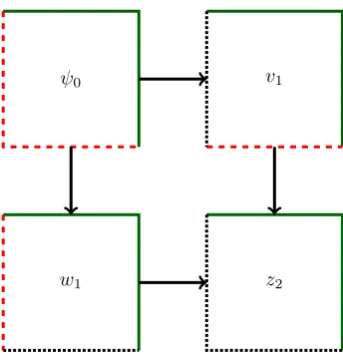
ψ0 v1

w1 z2

Figure 4.1: The interplay of Neumann corrections, solid line: no error, dashed line: error, densely-dotted line: correction

the situation for the first step for b_{= (b1, b2)∈}R2 _{withb1, b2>0, which we shall abbreviate by writing}

b_>0.

Let us start by definingψ0. It solves a reduced problem that can formally be found by comparing

powers ofεin the general approach (4.1). We have

(b_{· ∇)∆ψ0−c∆ψ0=f in Ω = (0,1)}2_{, (4.3a)}

ψ0= 0 on Γ =∂Ω, (4.3b)

∂nψ0= 0 on Γ−, (4.3c)

where Γ− :={(x, y)∈Γ| −b·n(x, y) <0} is the inflow boundary. According to Proposition 2.21 the

third-order problem (4.3) has a unique solution satisfying homogeneous Dirichlet conditions on the whole boundary Γ, and homogeneous Neumann conditions on the inflow boundary Γ− only. This is similar to

the asymptotic expansions for second order problems as in [13].

Now the normal derivative ofψ0 is in general non-zero on the outflow boundary. Thus, we correct

these Neumann data by correction functionsviinx-direction andwiiny-direction. We recall our standing

assumption ofb_{>0, the general case}b_{= (b1, b2) withb1·b26= 0 can be derived from the one with}b_>0 by a change of coordinates. Using b_{>0, we find the outflow boundary at x= 0 and y= 0. The layers} occur atx= 0 andy= 0 as well.

We will now define the correction function for the layer at x = 0. They can formally be derived with the help of the stretched variable ξ defined byξ= x

ε and comparison of powers ofε in the

trans-formed differential operator ˜L. We obtain ˜L expressed in terms of the variableξ andy by a coordinate transformation

˜

Lv˜(ξ, y) =ε−3˜vξξξξ+ 2ε−1v˜ξξyy+εv˜yyyy+ε−3b1v˜ξξξ+ε−1b1v˜ξyy+ε−2b2v˜ξξy+b2v˜yyy

−ε−2cv˜ξξ−c˜vyy

=ε−3(˜vξ+b1v˜)ξξξ+ε−2(b2v˜y−c˜v)ξξ+ε−1(2˜vξ+b1v˜)ξyy+ (b2v˜y−c˜v)yy+εv˜yyyy. (4.4)

Now the function v is to correct the Neumann data. Thus, it has to fulfil the boundary conditions at

x= 0, that isξ= 0. Therefore, we consider the Neumann derivative in x= 0 of the (formally) infinite sum (4.1) and make a comparison in the powers ofε. The last two sums are set to zero, because they do not have to correct anything. We get conditions on the functions ψi and ˜vi, namely

ψi,x(0, y) =−v˜i+1,ξ(0, y) (4.5)

for correcting the contributions of ψi to the Neumann data at x= 0. The functions ψi and ˜vi act on

different ε-levels because we consider the derivative of ˜vi in ξand thus, we get an additional order ofε.

Note that we do not correct the boundary conditions up to arbitrarily large values of i. We make use of this condition only for the considered finite number of indices. Additionally, the boundary correction functions are expected to be exponentially decaying away from the boundary. For this reason, we expand the domain of ˜Lfrom (0,1

Now, the boundary condition (4.5) shows that the contribution ofψ0 will be corrected byv1. Thus,

v0has nothing to correct and therefore we set

˜

v0= 0.

For ˜v1 the comparison of powers ofεin (4.4) with ˜L˜v= 0 yields

˜

v1,ξξξξ+b1v˜1,ξξξ=−b2v˜0,ξξy+c˜v0,ξξ= 0 in (0,∞)×(0,1),

˜

v1,ξ(0, y) =−ψ0,x(0, y) and lim

ξ→∞˜v1(ξ, y) = 0.

This problem has constant coefficients and no derivatives iny. Therefore, it can be solved explicitly and has the solution

˜

v1(ξ, y) = ψ0,x(0, y)

b1

exp{−b1ξ} or v1(x, y) = ψ0,x(0, y)

b1

E1(x).

Analogously, we obtain the correction function ˜w0= 0 and ˜w1(x, η) with the stretched variableη= y_ε for

the layer alongy= 0:

˜

w1(x, η) =

ψ0,y(x,0)

b2

exp{−b2η} or w1(x, y) =

ψ0,y(x,0)

b2

E2(y).

Both boundary correction functionsv1 andw1introduce non-zero Dirichlet and Neumann contributions

at the outflow-boundary. We correct the Neumann data by a corner correction function z2 and the

Dirichlet data by ψ1. For the corner-correction function we apply the stretching of the coordinates in

both directions and obtain formally the operator

¯

Lz¯(ξ, η) =ε−3_(¯z

ξξξξ+ 2¯zξξηη+ ¯zηηηη) +ε−3(b1(¯zξξξ+ ¯zηηξ) +b2(¯zξξη+ ¯zηηη))−ε−2c(¯zξξ+ ¯zηη).

Again, the correction function is to correct the Neumann data of v alongy = 0 (η= 0) and of w along

x= 0 (ξ= 0). Thus we have

˜

vi,y(ξ,0) =−z¯i+1,η(ξ,0) and w˜i,x(0, η) =−z¯i+1,ξ(0, η),

respectively. This time we obtain ¯z0= ¯z1= 0 because they have nothing to correct. The corner-correction

function ¯z2satisfies

¯

∆2z¯2+ (b·∇¯) ¯∆¯z2=c∆¯¯z1= 0 in (0,∞)×(0,∞),

¯

z2,η(ξ,0) =−v˜1,y(ξ,0) and ¯z2,ξ(0, η) =−w˜1,x(0, η),

lim

ξ→∞z¯2(ξ, η) = 0 and limη→∞z¯2(ξ, η) = 0.

A solution can be found to be

¯

z2(ξ, η) =−

ψ0,xy(0,0)

b1b2

exp{−b1ξ}exp{−b2η} or z2(x, y) =−

ψ0,xy(0,0)

b1b2

E1(x)E2(y).

As said before, the boundary-correction functionsv1 andw1 introduce non-neglectable contributions

in the Dirichlet data on Γ+:={(x, y)∈Γ :−b·n(x, y)>0}. This will be corrected in the next step by

ψ1 satisfying the reduced problem

(b_{· ∇)∆ψ1−c∆ψ1=−∆}2_{ψ0 in Ω = (0,1)}2_,

ψ1= 0 on Γ−,

∂nψ1(x, y) = 0 on Γ−,

ψ1(0, y) =−v1(0, y) y ∈(0,1),

ψ1(x,0) =−w1(x,0) x∈(0,1).

Now the construction of problems forv2 andw2 follows the same pattern as the construction forv1

andw1, respectively. We get

˜

v2(ξ, y) =

_ψ

1,x(0, y)

b1

−α(y) b3

1

−α(y)ξ b2

1

exp{−b1ξ},

that isv2(x, y) =

_ψ

1,x(0, y)

b1

−α(y) b3

1

−α(y)x b2

1ε

E1(x)

withα(y) =−b2ψ0,xy(0, y) +cψ0,x(0, y)

and

˜

w2(x, η) =

ψ1,y(x,0)

b2

−β(x) b3

2

−β(x)η b2

2

exp{−b2η},

that isw2(x, y) =

_ψ

1,y(x,0)

b2

−β(x) b3

2

−β(x)y b2

2ε

E2(y)

withβ(x) =−b1ψ0,xy(x,0) +cψ0,y(x,0).

The function ¯z3 has to fulfil the following problem:

¯ ∆2_z¯

3+ (b·∇¯) ¯∆¯z3=c∆¯¯z2=−

c(b2 1+b22)

b1b2

ψ0,xy(0,0) exp{−b1ξ}exp{−b2η} in (0,∞)×(0,∞),

¯

z3,η(ξ,0) =−v˜2,y(ξ,0) and z¯3,ξ(0, η) =−w˜2,x(0, η),

lim

ξ→∞z¯3(ξ, η) = 0 and ηlim→∞z¯3(ξ, η) = 0.

We make the ansatz

z3(ξ, η) = (ω1+ω2ξ+ω3η) exp{−b1ξ}exp{−b2η}

with unknown constantsω1, ω2, ω3. With this ansatz, we get only a solution if the compatibility condition

(b_{· ∇)ψ0,xy(0,0)−cψ0,xy(0,0) = 0 (4.6)} holds true. Then, the solution is given by

¯

z3(ξ, η) = (ω1+ω2ξ+ω3η) exp{−b1ξ}exp{−b2η} or z3(x, y) =

ω1+ω2

x ε +ω3

y ε

E1(x)E2(y)

with

ω1=

−b1b2ψ1,xy(0,0) +b1ψ0,xyy(0,0) +b2ψ0,xxy(0,0)

b2 1b22

,

ω2=

ψ0,xxy(0,0)

b1b2

and ω3=

ψ0,xyy(0,0)

b1b2

.

Without the explicit ansatz for z3 we also get several compatibility conditions, which follow from the

differential equation itself and the boundary conditions, warranting z3 to be continuous in the corner

(0,0).

Nowz2 introduces non-neglectable contributions in the Dirichlet data on Γ+. Thus for the next step,

ψ2 has to correct the Dirichlet data ofv2, w2 andz2. We consider the equation

(b_{· ∇)∆ψ2−c∆ψ2=−∆}2_{ψ1 in Ω = (0,1)}2_,

ψ2= 0 on Γ−,

∂nψ2= 0 on Γ−,

ψ2(0, y) =−v2(0, y)−w2(0, y)−z2(0, y) y∈(0,1),

ψ2(x,0) =−v2(x,0)−w2(x,0)−z2(x,0) x∈(0,1).

We again have to check the conditions of Proposition 2.21. Therefore, we have to verify, whether the following equations hold

−v2(0,1)−w2(0,1)−z2(0,1) = 0, (4.7a)

−v2(1,0)−w2(1,0)−z2(1,0) = 0, (4.7b)

−v2,y(0,1)−w2,y(0,1)−z2,y(0,1) = 0, (4.7c)

We begin with equation (4.7a):

v2(0,1) +w2(0,1) +z2(0,1)

= ψ1,x(0,1)

b1

−α(1) b3

1

+

ψ1,y(0,0)

b2

−β(0) b3

2

−β(0) b2

2ε

E2(1)−

ψ0,xy(0,0)

b1b2

E2(1)

=

− 2

b1b2

+b1

b3 2

+ b1

b2 2ε

ψ0,xy(0,0)E2(1) = 0.

This is zero, if

ψ0,xy(0,0) = 0. (4.8)

Equation (4.7b) yields

v2(1,0) +w2(1,0) +z2(1,0)

= _ψ

1,x(0,0)

b1

−α(0) b3

1

−α(0) b2

1ε

E1(1) +

ψ1,y(1,0)

b2

−β(1) b3

2

−ψ0,xy(0,0) b1b2 E1(1)

=

− 2

b1b2

+b2

b3 1

+ b2

b2 1ε

ψ0,xy(0,0)E1(1) = 0

and also gives condition (4.8). Let us continue with equation (4.7c):

v2,y(0,1) +w2,y(0,1) +z2,y(0,1)

=ψ1,xy(0,1)

b1

−αy(1) b3 1 + _−b 2 ε _ψ

1,y(0,0)

b2

−β(0) b3

2

−β(0) b2

2ε

−β(0)

b2 2ε

E2(1) +

ψ0,xy(0,0)

b1

E2(1)

(4.8)

= ψ1,xy(0,1)

b1

−αy(1) b3

1

−ψ1,y(0,0) ε E2(1)

=b2ψ0,xyy(0,1)

b3 1

= 0.

Analogously, we get for equation (4.7d)

v2,x(1,0) +w2,x(1,0) +z2,x(1,0) = b1ψ0,xxy(1,0)

b3 2

= 0.

Thus we obtain the additional conditions

ψ0,xyy(0,1) = 0 and ψ0,xxy(1,0) = 0. (4.9)

If the conditions (4.8) and (4.9) are violated, Proposition 2.21 is not applicable. Hence, it is unclear, whether a solution ψ2 exists. Condition (4.8) implies thatz2= 0.

Remark 4.1 From the conditions (4.9) we get conditions on f, namely f(0,1) = 0 and f(1,0) = 0. This follows by extension of the differential equation for ψ0 to the boundary. Furthermore, if b1 =b2,

condition (4.6) implies that f(0,0) = 0.

The construction ofv3 andw3 follows the same pattern as those forv1, v2, w1 andw2. The structure of

the solutions is of the form

˜

v3(ξ, y) =Pe2(ξ, y) exp{−b1ξ} or v3(x, y) =Pe2

_x

ε, y

E1(x),

˜

w3(x, η) =Qe2(x, η) exp{−b2η} or w3(x, y) =Qe2

x,y ε

E2(y),

wherePe2is a polynomial of second order in the first variable andQe2a polynomial of second order in the

second variable. To continue the expansion with higher order terms of ǫin the same manner results in more compatibility conditions. So, we stop the classical asymptotic expansion here. We add functions ˜

want them to satisfy:

˜

v4,ξξξξ+b1˜v4,ξξξ=−b2v˜3,ξξy+cv˜3,ξξ−2˜v2,ξξyy−b1v˜2,ξyy−b2v˜1,yyy+c˜v1,yy, in (0,∞)×(0,1),

˜

v4,ξ(0, y) = 0,in (0,1),

lim

ξ→∞v˜4(ξ, y) = 0,in (0,1),

˜

w4,ηηηη+b2w˜4,ηηη =−b1w˜3,xηη+cw˜3,ηη−2 ˜w2,xxηη−b2w˜2,xxη−b1w˜1,xxx+cw˜1,xx, in (0,1)×(0,∞),

˜

w4,η(x,0) = 0,in (0,1),

lim

η→∞w˜4(x, η) = 0,in (0,1),

¯

∆2z¯4+ (b·∇¯) ¯∆¯z4=c∆¯¯z3.

The boundary data of ¯z4only have to be bounded by a constant and need not to correct other data, thus

we have some freedem in the choice for ¯z4. We get

˜

v4(ξ, y) =Pe3(ξ, y) exp{−b1ξ} or v3(x, y) =Pe3

_x

ε, y

E1(x),

˜

w4(x, η) =Qe3(x, η) exp{−b2η} or w3(x, y) =Qe3

x,y ε

E2(y),

where ˜P3 is a polynomial of third order in the first variable and ˜Q3 a polynomial of third order in the

second variable. The function z4is of the structure

¯

z4(ξ, η) = ¯R2(ξ, η) exp{−b1ξ}exp{−b2η} or z4(x, y) = ¯R2

_x

ε, y ε

E1(x)E2(y),

where ¯Ris a polynomial of second order in both variables.

4.2

Estimating the residual

Consider now the approximation Ψ ofψgiven by

Ψ =

2

X

i=0

εiψi+

4

X

i=1

εivi+

4

X

i=1

εiwi+

4

X

i=2

εizi,

with the functions given before. Furthermore, letR=ψ−Ψ be the residual of the solution of problem (1.1) and its approximation Ψ. We now estimate the residualRwith the help of Theorem 3.3. Let us start with some lemmas. In all the lemmas, it is implicitly assumed that the compatibility conditions (4.6), (4.8) and (4.9) are fulfilled. We also recall our standing assumption on the solutions to be sufficiently smooth.

Lemma 4.2 For the residualR holds

kLRkL2_(Ω)≤Cε5/2. (4.10)

Proof

Let us start by computing

LR=L(ψ−ψ0−εψ1−ε2ψ2−εv1−ε2v2−ε3v3−ε4v4−εw1−ε2w2−ε3w3−ε4w4

−ε2z2−ε3z3−ε4z4)

=L(ψ−ψ0−εψ1−ε2ψ2)−L(εv1+ε2v2+ε3v3+ε4v4)

−L(εw1+ε2w2+ε3w3+ε4w4)−L(ε2z2+ε3z3+ε4z4). (4.11)

We obtain for the first term of (4.11)

L(ψ−ψ0−εψ1−ε2ψ2) =f−f+ε∆2ψ0−ε∆2ψ0+ε2∆2ψ1−ε2∆2ψ1+ε3∆2ψ2

=ε3∆2ψ2.

For the second term of (4.11) we have

L(εv1+ε2v2+ε3v3+ε4v4) = ˜L(εv˜1+ε2v˜2+ε3˜v3+ε4˜v4)

=ε2_((˜v

1,yy+b2˜v2,y−cv˜2+ 2˜v3,ξξ+b1˜v3,ξ)yy+ (b2v˜4,y−cv˜4)ξξ)

+ε3(˜v2,yy+b2˜v3,y−cv˜3+ 2˜v4,ξξ+b1˜v4,ξ)yy

The third term of (4.11) can be rewritten analogously. Finally, the remaining term in (4.11) is

L(ε2z2+ε3z3+ε4z4) = ¯L(ε2z¯2+ε3z¯3+ε4z¯4)

=−ε2c∆¯¯z4.

Thus, we obtain with some functions g1, g2, g3that are bounded independently of ε

LR(x, y) =ε3∆2ψ2(x, y) +ε2(g1(y)E1(x) +g2(x)E2(y) +g3(x, y)E1(x)E2(y)) (0≤x, y≤1),

which yields (4.10).

Lemma 4.3 The residualR can be bounded on the boundaryΓ =∂Ωby

kRkL∞_(Γ)≤Cε3. (4.12)

Its tangential derivative ∂t is bounded on∂Ωby

k∂tRkL∞_(Γ)≤Cε2. (4.13)

Proof

We will give details only for some of the terms occuring in the expression forR as the estimates for the others follow the same rationale. Let us start out with

R(1, y) =ψ(1, y)−ψ0(1, y)−εψ1(1, y)−ε2ψ2(1, y)

−ε(v1(1, y) +w1(1, y))−ε2(v2(1, y) +w2(1, y) +z2(1, y))

−ε3_(v

3(1, y) +w3(1, y) +z3(1, y))−ε4(v4(1, y) +w4(1, y) +z4(1, y))

The first four terms of R(1, y) are zero, because these functions fulfil homogeneous Dirichlet boundary conditions.

The correction terms with index 1 yield

v1(1, y) +w1(1, y) = ψ0,x(0, y)

b1

E1(1) +ψ0,y(1,0)

b2

E2(0) = ψ0,x(0, y)

b1

E1(1)

because ψ0,y(1,0) = 0 due to homogeneous Dirichlet boundary conditions of ψ0. The factor E1(1) is

exponentially small in ε and can therefore be bounded by an arbitrary power ofε. For the corrections with index 2 we have

w2(1, y) =

ψ1,y(1,0)

b2

−β(1) b3

2

−β(1)y b2

2ε

E2(y) = 0

because β(1) = 0 due to ψ0,xy(1,0) = 0 and ψ1,y(1,0) = 0 due to homogeneous Dirichlet boundary

conditions ofψ1, and

v2(1, y) +z2(1, y) =v2(1, y) =

_ψ

1,x(0, y)

b1

−α(y) b3

1

−α(y) b2

1ε

E1(1).

We obtain for the corrections with index 3

v3(1, y) +z3(1, y) =Pe2

x=1

ε, y

E1(1) + ¯R1

x= 1

ε, y ε

E1(1)E2(y).

Finally,

w3(1, y) =Qe2

1,y

ε

E2(y)

is bounded by a constant due to P2(t)e−t ≤ C for all t, where P2 is a polynomial of order 2. The

corrections with index 4 contribute similar bounds as an analogous argument shows. Combining the terms discussed so far, we obtain with some function g, bounded independently of ε, and polynomials

P2, P3,

R(1, y) =εg(y)E1(1) +

ε3P2

_y

ε

+ε4P3

_y

ε

E2(y), (0≤y≤1).

Thus, theL∞_{-norm over this part of the boundary is bounded by}

Let us take a look at the outflow boundary at x= 0. Here, we do not have an arbitrarily small factor

E1(1) in our estimates. We start with

R(0, y) =ψ(0, y)−ψ0(0, y)−εψ1(0, y)−ε2ψ2(0, y)

−ε(v1(0, y) +w1(0, y))−ε2(v2(0, y) +w2(0, y) +z2(0, y))

−ε3(v3(0, y) +w3(0, y) +z3(0, y))−ε4(v4(0, y) +w4(0, y) +z4(0, y)).

The first two terms are zero due to the imposed Dirichlet conditions. By definition ofψ1andψ2 we have

ψ1(0, y) =−v1(0, y),

ψ2(0, y) =−v2(0, y)−w2(0, y)−z2(0, y).

Employing the fact that w1(0, y) is zero sinceψ0 satisfies homogeneous Dirichlet conditions and, hence,

ψ0,y(0,0) = 0, we get

R(0, y) =−ε3(v3(0, y) +w3(0, y) +z3(0, y))−ε4(v4(0, y) +w4(0, y) +z4(0, y)).

We obtain with the same methods as above for some function hbounded independently ofε and poly-nomialsP2, P3,

R(0, y) =ε3h(y) +P2

_y

ε

+εP3

_y

ε

E2(y)

(0≤y≤1).

Thus, theL∞_{-norm of this part of the boundary is also bounded by}

kR(0,·)kL∞_(0,1)≤Cε3.

On the remaining boundaries we use similar ideas and eventually obtain (4.12). For the tangential derivative we estimateRy(0, y) andRy(1, y): We obtain

kRy(0,·)kL∞

(0,1)≤Cε2 and kRy(1,·)kL∞

(0,1)≤Cε2

due toE2,y(y) =−b_ε2E2(y). On the other boundaries we apply the same techniques and conclude (4.13).

Lemma 4.4 The normal derivative ofR on the boundary∂Ωcan be estimated by

k∂nRk_L∞

(Γ)≤Cε3 andk∂nRk_L2_(Γ)≤Cε

7/2_{. (4.14)}

Proof

Again, we only exemplify the method of proof. The terms not discussed are estimated using the same techniques. Let us start out with R(1, y). Here, we have

Rx(1, y) =ψx(1, y)−ψ0,x(1, y)−εψ1,x(1, y)−ε2ψ2,x(1, y)

−ε(v1,x(1, y) +w1,x(1, y))−ε2(v2,x(1, y) +w2,x(1, y) +z2,x(1, y))

−ε3(v3,x(1, y) +w3,x(1, y) +z3,x(1, y))−ε4(v4,x(1, y) +w4,x(1, y) +z4,x(1, y)).

Now,

ψx(1, y)−ψ0,x(1, y)−εψ1,x(1, y)−ε2ψ2,x(1, y) = 0

due to the homogeneous Neumann boundary conditions at this boundary of the functions ψ, ψ0, ψ1 and

ψ2. For the next terms we have

v1,x(1, y) +w1,x(1, y) =−

ψ0,x(1, y)

ε E1(1) +

ψ0,xy(1, y)

b2 E2(y)

=−ψ0,x(1, y) ε E1(1)

because ψ0 satisfies homogeneous Neumann boundary condition alongx= 1 and, hence, itsy-derivative

is zero. The terms with index 2 are

w2,x(1, y) =

_ψ

1,xy(1,0)

b2

−βx(1) b3

2

−βx(1)y b2

2ε

E2(y)

=b1ψ0,xxy(1,0)

b3 2

1 +b2y

ε

due to the compatibility condition (4.9), and

v2,x(1, y) +z2,x(1, y) =−

b1

ε

ψ1,y(1,0)

b1

−α(y) b3

1

−α(y) b2

1ε

E1(1).

The terms with index 3 contribute

v3,x(1, y) +z3,x(1, y) =

˜

P2,x

₁

ε, y

−b1

εP˜2

₁

ε, y

+w2

ε E2(y)− b1

ε

ω1+ω2

1

ε +ω3 y ε

E2(y)

E1(1)

and

w3,x(1, y) = ˜Q2,x

1,y

ε

E2(y)

which is bounded by a constant due toP2(t)e−t≤C for allt, whereP2 is a polynomial of order 2. The

same arguments apply to the correction functions with index 4. Combining all these terms, we have for some functiong bounded independently ofεand constantsc7, c8 andc9 independent ofε

Rx(1, y) =g(y)E1(1) +ε3

c7+c8

_y

ε

+c9

_y

ε

2

E2(y).

Thus, we obtain

kRx(1,·)kL∞

(0,1)≤Cε3 and kRx(1,·)kL2_(0,1)≤Cε7/2.

On the outflow boundary atx= 0 we have

Rx(0, y) =ψx(0, y)−ψ0,x(0, y)−εψ1,x(0, y)−ε2ψ2,x(0, y)

−ε(v1,x(0, y) +w1,x(0, y))−ε2(v2,x(0, y) +w2,x(0, y) +z2,x(0, y)

−ε3(v3,x(0, y) +w3,x(0, y) +z3,x(0, y))−ε4(v4,x(0, y) +w4,x(0, y) +z4,x(0, y)).

The first term is zero and the next terms cancel with their corresponding layer-correction functions. So far, we have

Rx(0, y) =−ε3w3,x(0, y)−ε4(v4,x(0, y) +w4,x(0, y) +z4,x(0, y)).

The remaining terms are not vanishing and we have for some functionhbounded independently ofεand constantsc10, c11andc12 independent ofε

Rx(0, y) =ε4h(y) +ε3

c10+c11

_y

ε

+c12

_y

ε

2

E2(y).

Thus, we obtain again

kRx(0,·)kL∞_(0,1)≤Cε3 and kR_x(0,·)k_L2_(0,1)≤Cε7/2.

The normal derivative on the other sides can be estimated similarly and we obtain (4.14).

We summarize the results obtained so far in the next proposition. Recall that we assumed sufficiently smooth solutions to be existent.

Proposition 4.5 Assume the compatibility conditions (4.6),(4.8)and (4.9)to be satisfied. We consider

the approximation of ψ given by

Ψ =

2

X

i=0

εiψi+

4

X

i=1

εivi+

4

X

i=1

εiwi+

4

X

i=2

εizi.

Then, the residualR=ψ−Ψcan be estimated by

kRkL∞_(Ω)≤Cε3/2 and kRk_H1_(Ω)≤Cε3/2.

Proof

We make use of Theorem 3.3. For this, using Lemmas 4.2, 4.3, 4.4, we are left with an estimate of the

C1/2_{-norm on Γ ofR. But, with the help of the estimates in both theC}1_{- andL}∞_{-norm it follows that}

kRkC1/2_(Γ)≤Cε5/2.

Theorem 4.6 Assume the compatibility conditions (4.6),(4.8)and (4.9)to be satisfied. Then the solu-tionψ of (1.1)can be decomposed in a regular partS and two layer parts in the following form:

ψ(x, y) =S(x, y) +εH(x, y)E1(x) +εI(x, y)E2(y), (0≤x, y≤1)

where the functionsS, H andI are independently bounded of ε.

Proof

The result follows from the asymptotic expansion which was done in this section. Proposition 4.5 yields that the residual Ris small enough and thus, it can be incorporated into the smooth part S due to the structure of the layer correcting terms. The corner layer partsz3 and z4 are also incorporated into the

smooth part.

Remark 4.7 The layers of ψ are so-called weak layers. If we look at ψ−S, with S being given by Theorem 4.6, we obtain

kψ−SkL∞

(Ω)≤Cε,

but

k∇(ψ−S)kL∞_(Ω)≤C,

that is the layers are visible in the first derivative forε→0.

4.3

Asymptotic expansion without compatibility conditions

With the rationale presented, we have seen that an asymptotic expansion of arbitrary order is possible upon imposing certain compatibility conditions. In fact, for the construction of ψ2 we needed (4.8) and

(4.9) to be satisfied. We make now an asymptotic expansion without any compatibility conditions and demonstrate that we will lose an ε-order in the estimates of the residualR, while we keep in mind that we assume the solutions occuring to be sufficiently smooth.

We keep the construction of the functionsψ0, ψ1, v1, w1, v2, w2 andz2. In the next step, we formally

set ψ2 = 0. This implies that we impose homogeneous boundary conditions for v3 and w3. For z3 we

choose an arbitrary, exponentially decaying function that fulfils a corner-correction type problem, given by

¯

∆2z¯3+ (b·∇¯) ¯∆¯z3=c∆¯¯z2

=−cψ0,xy(0,0) exp{−b1ξ}exp{−b2η}(b

2 1+b22)

b1b2

in (0,∞)×(0,∞).

Its boundary data only have to be bounded by a constant and need not to correct other data, thus we have some freedom in choosing ¯z3. We take

z3(x, y) = cψ0,xy(0,0)

b1b2(b1+b2)

_x

ε+ y ε

E1(x)E2(y).

Next, we consider an approximation Ψnew _{ofψ given by}

Ψnew=ψ0+εψ1+εv1+ε2v2+ε3v3+εw1+ε2w2+ε3w3+ε2z2+ε3z3.

Following the strategies exemplified in the previous section, we derive estimates for the new residual.

Lemma 4.8 For the residualRnew _=ψ−Ψnew _{we get the following estimates:}

kLRnew_k

L2_(Ω)≤Cε3/2,

kRnewkL∞

(Γ)≤Cε2, k∂tRnewkL∞

(Γ)≤Cε,

k∂nR

new_k

L∞_(Γ)≤Cε2, k∂_nRnewk_L2_(Γ)≤Cε5/2

and finally

kRnewkL∞_(Ω)≤Cε1/2. Proof

So we see that theε-order of the residualRnew _{is not small enough to have a solution decomposition like}

in Theorem 4.6. We can only show the following.

Proposition 4.9 Consider equation (1.1). The solutionψ can be represented as

ψ(x, y) =S(x, y) +εH(x, y)E1(x) +εI(x, y)E2(y) +ε2J(x, y)E1(x)E2(y) +Rnew(x, y), (0≤x, y≤1)

where the functionsS, H, I, J are bounded independently of εand the residual is of orderε1/2_.

Acknowledgement

We would like to thank J¨urgen Rossmann for his help with providing a stability result for the solution of singularly perturbed fourth-order problems, see Theorem 3.3.

This work was supported by the German Research Foundation (DFG) under Project No. FR 3052/2-1.

References

[1] R. A. Adams and J. J. F. Fournier. Sobolev spaces, volume 140 of Pure and Applied Mathematics

(Amsterdam). Elsevier/Academic Press, Amsterdam, second edition, 2003.

[2] H. Blum and R. Rannacher. On the boundary value problem of the biharmonic operator on domains with angular corners. Math. Methods Appl. Sci., 2(4):556–581, 1980.

[3] S. C. Brenner and L.-Y. Sung. C0_{interior penalty methods for fourth order elliptic boundary value}

problems on polygonal domains. J. Sci. Comput., 22-23(1-3):83–118, 2005.

[4] E. M. de Jager and J. Furu.The theory of singular perturbations, volume 42 ofNorth-Holland Series

in Applied Mathematics and Mechanics. North-Holland Publishing Co., Amsterdam, 1996.

[5] G. Engel, K. Garikipati, T.J.R. Hughes, M.G. Larson, L. Mazzei, and R.L. Taylor. Continu-ous/discontinuous finite element approximations of fourth-order elliptic problems in structural and continuum mechanics with applications to thin beams and plates, and strain gradient elasticity.

Computer Methods in Applied Mechanics and Engineering, 191(34):3669–3750, 2002.

[6] A. Ern and J.-L. Guermond. Theory and practice of finite elements, volume 159 ofApplied

Mathe-matical Sciences. Springer-Verlag, New York, 2004.

[7] S. Franz, H.-G. Roos, and A. Wachtel. A C0 _{interior penalty method for a singularly-perturbed}

fourth-order elliptic problem on a layer-adapted mesh. Numer. Methods Partial Differential

Equa-tions, 30(3):838–861, 2014.

[8] J. Guzm´an, D. Leykekhman, and M. Neilan. A family of non-conforming elements and the analysis of nitsches method for a singularly perturbed fourth order problem. Calcolo, 49(2):95–125, 2012. [9] T. Kato.Perturbation theory for linear operators. Springer-Verlag, Berlin-New York, second edition,

1976. Grundlehren der Mathematischen Wissenschaften, Band 132.

[10] R. B. Kellogg and M. Stynes. Sharpened and corrected version of: Corner singularities and boundary layers in a simple convection-diffusion problem. J. Differential Equations, 213(1):81–120, 2005. [11] R. B. Kellogg and M. Stynes. Sharpened bounds for corner singularities and boundary layers in a

simple convection-diffusion problem. Appl. Math. Lett., 20(5):539–544, 2007.

[12] V. A. Kozlov, V. G. Maz′_{ya, and J. Rossmann. Elliptic boundary value problems in domains with}

point singularities, volume 52 ofMathematical Surveys and Monographs. American Mathematical

Society, Providence, RI, 1997.

[13] T. Linß and M. Stynes. Asymptotic analysis and Shishkin-type decomposition for an elliptic convection-diffusion problem. J. Math. Anal. Appl., 261(2):604–632, 2001.

[14] V. G. Maz′_{ya and J. Rossmann. On the Agmon-Miranda maximum principle for solutions of elliptic}

[15] J. Neˇcas. Direct methods in the theory of elliptic equations. Springer Monographs in Mathematics. Springer, Heidelberg, 2012. Translated from the 1967 French original by Gerard Tronel and Alois Kufner, Editorial coordination and preface by ˇS´arka Neˇcasov´a and a contribution by Christian G. Simader.

[16] J. Rossmann. Personal Communication, June 2015.

[17] G. F. Sun and M. Stynes. Finite-element methods for singularly perturbed high-order elliptic two-point boundary value problems. II. Convection-diffusion-type problems. IMA J. Numer. Anal., 15(2):197–219, 1995.

[18] H. Triebel. Interpolation theory, function spaces, differential operators. 2nd rev. a. enl. ed. Leipzig: Barth, 2nd rev. a. enl. ed. edition, 1995.

[19] S. Trostorff and M. Waurick. A note on elliptic type boundary value problems with maximal mono-tone relations. Math. Nachr., 287(13):1545–1558, 2014.

[20] O. S. Zikirov. A non-local boundary value problem for third-order linear partial differential equation of composite type. Math. Model. Anal., 14(3):407–421, 2009.