A spline method for solving fourth order singularly perturbed boundary
value problem
Talat Sultana
∗Department of Mathematics, Janki Devi Memorial College, University of Delhi, New Delhi-60, INDIA.
Abstract
In this paper, singularly perturbed boundary value problem of fourth order ordinary differential equation with a small positive parameter multiplying with the highest derivative of the form
εu(4)(x) +p(x)u
00
(x) +q(x)u(x) =r(x), 0≤x≤1,
u(0) =γ0,u(1) =γ1,u
00
(0) =η0,u
00
(1) =η1, 0≤ε≤1
is considered. We have developed a numerical technique for the above problem using parametric and poly-nomial septic spline method. The method is shown to have second and fourth order convergent depending on the choice of parameters involved in the method. Truncation error and boundary equations are obtained. The method is tested on an example and the results are found to be in agreement with the theoretical analysis.
Keywords: Parametric septic splines, Polynomial septic splines, Boundary value problems, Boundary equations.
2010 MSC:65D07, 65L10, 65L11. c2012 MJM. All rights reserved.
1
Introduction
Singular perturbation problems appear in many branches of applied mathematics, and for more than two decades quite a large number of research papers on the qualitative and quantitative analysis of these problems for both ordinary differential equations (ODEs) and partial differential equations (PDEs) have been reported in the literature. Most of the papers connected with computational aspects are confined to second order equations. But only few authors have developed numerical methods for singularly perturbed higher order differential equations. These problems are classified on the basis of how the order of original differential equa-tion is affected if setsε=0 [8]. Here,εis a small positive parameter multiplying with the highest derivative
of the differential equation. The singularly perturbed problem is of convection-diffusion type if the order of the differential equation is reduced by 1, whereas it is called reaction-diffusion type if order is reduced by 2. The objective of the present paper is to develop a computational method to solve singularly perturbed bound-ary value problems of fourth order ordinbound-ary differential equations of the form:
εu(4)(x) +p(x)u
00
(x) +q(x)u(x) =r(x), 0≤x≤1,
u(0) =γ0,u(1) =γ1,u
00
(0) =η0,u
00
(1) =η1, 0≤ε≤1,
(1.1)
where p(x), q(x)andr(x)are smooth, bounded, real functions p(x): R → R, q(x) : R→ R, r(x) : R → R
satisfying the following conditions
−p≥β>0, 0≥q≥ −γ,γ>0,
∗Corresponding author.
β−2γ≥η>0, f or some η,
D= (0, 1),D= [0, 1]and ueC4(D)
\
C2(D). (1.2)
Analytical and numerical treatment of these equations have drawn much attention of many authors [5,22-25]. The analytical treatment of singularly perturbed boundary value problems for higher order nonlinear ordinary differential equations, which have important applications in Fluid Dynamics, can be found in [1,2,6-9,13,20]. Semper [2] and Roos and Stynes [8] considered fourth order equations and applied a standard finite element method. Garland [3] has shown that uniform stability of discrete boundary value problem follows from uniform stability of the discrete initial value problem and uniform consistency of the scheme. Some re-sults connected with the exponentially fitted higher order differences with identity expansion method [3] and defect corrections are available in the literature. Loghmani and Ahmadinia [5] have developed a numerical technique for solving singularly perturbed boundary value problems based on optimal control strategy by using B-spline functions and least square method. Also finite element method is reported in [6,7]. In [9], an iterative method is described. In [10,11,16,17,20], the authors have applied boundary value technique to find the numerical solution for singularly perturbed second order boundary value problems. Niederdrenk and Yserentant [12] considered convection diffusion type problems and derived conditions for the uniform stabil-ity of discrete and continuous problems. Feckan [13] considered higher order problems and his approach is based on the nonlinear analysis involving fixed point theory, Leray-Schauder theory etc. In [15], authors have given a brief survey on computational techniques for the different classes of singularly perturbed problems. Bawa [19] and Aziz and Khan [21] have solved second order singularly perturbed boundary value problem using spline technique. Shanthi and Ramanujam [22-25] have developed numerical methods for singularly perturbed higher order boundary value problems.
In this problem, we takep(x) =p=constant andq(x) =q=constant. In the present paper, parametric septic spline is described for fourth order boundary value problems. In section 2, a brief description of the method is given. Development of the boundary equations are given in section 3. In section 4, truncation error and class of methods are discussed. We established the convergence of our method in section 5 and section 6 contains the numerical results and discussions.
2
Derivation of the method
In order to develop the numerical method for approximating the solution of singularly perturbed fourth order boundary value problem, the interval[0, 1]is divided intoNequal subintervals using the grid points
xj =jh, j=0(1)N, where
x0=0, xN=1, and h= 1
N. (2.1)
A functionS∆(x,τ)of classC6[0, 1]which interpolatesu(x)at the mesh pointxj depends on a parameterτ,
and asτ→0 it reduces to septic splineS∆(x)in[0, 1]is termed as parametric septic spline function. Since the
parameterτcan occur inS∆(x)in many ways such a spline is not unique.
IfS∆(x,τ) =S∆(x)is a piecewise function satisfying the following differential equation in the interval[xj−1,xj]
S(6)∆ (x)−τ2S
00
∆(x) = (Qj−τ2Mj)
x−xj−1
h + (Qj−1−τ
2M
j−1)
xj−x h
= Ajz+Aj−1z¯,
(2.2)
where
z= x−xj−1
h , z=1−z, Ak =Qk−τ
2M
k,S
00
∆(xk,τ) =Mk, S∆(6)(xk,τ) =Qk, k=j−1,j; τ>0,
then it is termed as parametric septic spline II. Solving equation (2.2), we get
S4(x) =B1+B2x+B3cosh
√
τx+B4sinh
√
τx+B5cos
√
τx+B6sin
√
τx
− 1
τ2
(
(Qj−τ2Mj)
(x−xj−1)3
6h + (Qj−1−τ
2Mj −1)
(xj−x)3 6h
)
To develop the consistency relations between the value of spline and its derivatives at knots, let
S∆(xj) =uj, S∆(xj+1) =uj+1,
S00∆(xj) =Mj, S00∆(xj+1) = Mj+1,
S(4)∆ (xj) =Fj, S(4)∆ (xj+1) =Fj+1.
(2.4)
To define spline in terms ofuj’s,Mj’s andFj’s, the coefficients introduced in Eq.(2.3) are calculated as
B1 = uj−1+ h 2 6τ2
(Qj−1−τ2Mj−1)−
Fj−1
τ2
−xj−1 h
(uj−uj−1)− h 2 6τ2
(Qj−1−τ2Mj−1) + h 2 6τ2
(Qj−τ2Mj) + 1 τ2
(Fj−1−Fj)
,
B2 = 1
h(uj−uj−1) + h
6τ2
−(Qj−1−τ2Mj−1) + (Qj−τ2Mj)
+ 1
τ2h
(Fj−1−Fj),
B3 = 1
τ2sinh
√ τh 1 2sinh √
τxj
Fj−1−
Qj−1
τ
−1
2sinh
√
τxj−1
Fj− Qj τ −1 τsinh √
τxj−1Qj+
1
τsinh
√
τxjQj−1
,
B4 = 1
τ2sinh
√ τh −1 2cosh √ τxj
Fj−1−
Qj−1 τ +1 2cosh √
τxj−1
Fj−Qj
τ
+1
τcosh
√
τxj−1Qj−
1
τcosh
√
τxjQj−1
,
B5 = 1
2τ2sinh
√
τh
sin√τxj
Fj−1−
Qj−1
τ
−sin√τxj−1
Fj− Qj
τ
,
B6 = 1
2τ2sinh
√
τh
−cos√τxj
Fj−1−
Qj−1
τ
+cos√τxj−1
Fj−Qj
τ
.
(2.5)
Substituting these values in (2.3), we get
S∆(x) = zuj+zuj¯ −1+h 2 6
p(z)Mj+p(z¯)Mj−1
+h 4 2
r(z)Fj+r(z¯)Fj−1
+h 6 6
q(z)Qj+q(z¯)Qj−1
,
(2.6)
where
p(z) =z3−z, q(z) = z
ω4 −
z3
ω4
+ 3 sinhωz
ω6sinhω −
3 sinωz ω6sinω,
r(z) = −2z
ω4 +
sinhωz ω4sinhω +
sinωz ω4sinω, ω=
√
τh. (2.7)
Applying the first, third and fifth derivative continuities at the knots, i.e.S(∆µ)(x−j ) =S∆(µ)(x+j ), µ=1, 3and5,
the following consistency relations are derived:
Mj+1+4Mj+Mj−1 = 6
h2(uj+1−2uj+uj−1) +3h 2(
α2Fj+1+2β2Fj+α2Fj−1)
+h4(α1Qj+1+2β1Qj+α1Qj−1), j=1(1)N−1, (2.8)
Mj+1−2Mj+Mj−1 = h 2 6 [(1−ω
4
α1)Fj+1+2(2−ω4β1)Fj+ (1−ω4α1)Fj−1]
−h
4
h2[(1−ω4α1)Qj+1+2(2−ω4β1)Qj+ (1−ω4α1)Qj−1] =
3[(ω4α2+2)Fj+1+2(ω4β2−2)Fj+ (ω4α2+2)Fj−1], j=1(1)N−1, (2.10) where
α1= 1
ω4 +
3
ω5sinhω−
3
ω5sinω, β1=
2
ω4 −
3
ω5cothω+
3
ω5cotω, α2=
−2
ω4
+ 1
ω3sinhω
+ 1
ω3sinω, β2
= 2
ω4
− 1
ω3cothω
− 1
ω3cotω.
(2.11)
Asτ→0 that isω→0 then(α1,β1,α2,β2)→(2520−31,315−4,1807 ,452). Using equations (2.8)-(2.10), we obtain the following scheme
(e1uj−3+e2uj−2+e3uj−1+e4uj+e3uj+1+e2uj+2+e1uj+3)
= h 4
6 (p1Fj−3+p2Fj−2+p3Fj−1+p4Fj+p3Fj+1+p2Fj+2+p1Fj+3),j=3(1)N−3, (2.12) where the coefficients(e1,e2,e3,e4)and(p1,p2,p3,p4)of the developed scheme are given by
e1 = 1−3ω4α1+3ω8α21−ω12α31,
e2 = 4ω4α1−2ω4β1−8ω8α21+4ω8α1β1−2ω12α21β1,
e3 = 7(1−ω4α1)3−8(1−ω4α1)2(2−ω4β1),
e4 = 12(1−ω4α1)2(2−ω4β1)−8(1−ω4α1)3,
p1 = c1(1−ω4α1)2,
p2 = 2c1(1−ω4α1)(2−ω4β1) +c2(1−ω4α1)2−3d1(1−ω4α1)(2+ω4α2),
p3 = (c1+c3)(1−ω4α1)2+6d1(1−ω4α1)(2−ω4β2) +2c2(1−ω4α1)(2−ω4β1)
−3d2(1−ω4α1)(2+ω4α2),
p4 = 2c2(1−ω4α1)2−6d1(1−ω4α1)(2+ω4α2)−6d1(2−ω4β1)(2−ω4β2) +2c3(1−ω4α1)(2−ω4β1) +6d2(1−ω4α1)(2−ω4β2).
(2.13)
Also
c1 = 1 6ω
8
α21−3
2ω 4
α22−1
3ω 4
α1−6α1−6α2+ 1 6,
c2 = 2 3ω
8
α21+1
3ω 8
α1β1−18ω4α1α2−3ω4α2β2−6ω4α22−2ω4α1− 1 3ω
4
β1−12α1−6β2+ 4 3,
c3 = 1 3ω
8
α21+4
3ω 8
α1β1−36ω4α1β2−12ω4α2β2−3ω4α22−10
3 ω 4
α1− 4 3ω
4
β1+36α1 +12α2+12β2+3,
d1 = ω4α2β1−ω4α1β2+6ω4α21−10α1−2α2+2β1+β2,
d2 = 4ω4α2β1−4ω4α1β2+12ω4α1β1−16α1−18α2−4β1+4β2.
(2.14)
Asτ→0 that isω→0, we have
(i)(e1,e2,e3,e4)−→(1, 0,−9, 16), (ii)(c1,c2,c3,d1,d2)−→
1
140,1714,24970,1409 ,354
,
(iii)(p1,p2,p3,p4)−→
1
140,67,1191140,60435
.
[Remarks:] For these values our scheme reduces to the polynomial septic spline for fourth order boundary value problem which is given as equation (7) in G. Akram and S. S. Siddiqi [4].
We have taken(e1,e2,e3,e4) = (1, 0,−9, 16)in Eq. (2.12) and obtained
p1(Fj−3+Fj+3) +p2(Fj−2+Fj+2) +p3(Fj−1+Fj+1) +p4Fj=
6
Eq. (1.1) can be written in the following form by takingp(x) =pandq(x) =qas
εFj+pMj+quj=rj. (2.16)
OperateΛxon the both side of Eq. (2.16), we get
εΛxFj+pΛxMj+qΛxuj=Λxrj (2.17)
where operatorΛxis defined as follows for any function0W0evaluated at mesh point
ΛxWj=p1(Wj−3+Wj+3) +p2(Wj−2+Wj+2) +p3(Wj−1+Wj+1) +p4Wj. (2.18)
For second derivative ofu, we take relation from [Eq. (5), Ref. [4]]
ΛxMj=
42
h2[(uj−3+uj+3) +24(uj−2+uj+2) +15(uj−1+uj+1)−80uj]. (2.19) Here,(p1,p2,p3,p4) = (1, 120, 1191, 2416)for second derivative. Using (2.15-2.19), we get
(6ε+42ph2+qh4p1)(uj−3+uj+3) + (1008ph2+qh4p2)(uj−2+uj+2)
+(−54ε+630ph2+qh4p3)(uj−1+uj+1) + (96ε−3360ph2+qh4p4)uj
=h4[p1(rj−3+rj+3) +p2(rj−2+rj+2) +p3(rj−1+rj+1) +p4rj], j=3(1)(N−3). (2.20)
3
Development of boundary equations
The relation (2.20) gives(N−5)algebraic equations in(N−1)unknownsuj,j =1(1)N−1. We require four more equations, two at each end of range of integartion in order to have closed form solution foruj. For the discretization of the boundary conditions, we have developed boundary equations for second and fourth order methods as follows:
3.1
Second order method
(i) −5u1+4u2−u3=−2γ0+h2η0−11h
4
12ε(r0−qγ0−pη0),j=1,
(ii) 525u1−575u2+285u3−1011u4= 72γ0−65h2η0,j=2,
(iii) −1110uN−4+285uN−3−575uN−2+525uN−1= 72γ1−56h2η1,j=N−2, (iv) −uN−3+4uN−2−5uN−1=−2γ1+h2η1−11h
4
12ε (rN−qγ1−pη1),j=N−1.
3.2
Fourth order method
(i) −132235 u1+11066245 u2−6684245u3+2171245u4−302245u5=−42935 γ0+20449h2η0−274h
4
245ε (r0−qγ0−pη0),j=1,
(ii) −1342
97 u1+7213375u2−2049146u3+3799691u4−1105912203u5+855112 u6=−98982449γ0+348323h2η0,j=2,
(iii) 855112 uN−6−1105912203uN−5+3799691uN−4−2049146uN−3+7213375uN−2−134297 uN−1=−98982449γ1+348323h2η1,j=N−2, (iv)−1322
35 uN−1+11066245 uN−2−6684245uN−3+2171245uN−4−302245uN−5=−42935γ1+20449h2η1−274
h4
245ε (rN−qγ1−pη1),j=
4
Truncation error
To obtain the local truncation error tj, j = 3(1)(N−3), associated with the scheme (2.20), substitute
rj = εu(4)j +pu
00
j +quj in eq. (2.20) and expanding it by Taylor series about xj, we obtain the following
lo-cal truncation error
tj = (864−48p1−48p2−48p3−24p4)
εh4
4! u (4)
j
+(8640−6480p1−2880p2−720p3)
εh6
6! u (6)
j
+(78624−272160p1−53760p2−3360p3)
εh8
8! u (8)
j −
6720 8! ph
10u(8)
j
+(708480−7348320p1−645120p2−10080p3)εh 10 10!u
(10)
j
+10080 10! ph
12u(10)
j +O(h12).
(4.1)
By using the above equation and eliminating the coefficients of various powers ofh, we can obtain class of the methods. For arbitrary choices ofp1,p2,p3andp4, we obtain the following methods:
4.1
Second order methods
By equating the coefficient ofh4equal to zero in (4.1), we get second order methods. Therefore,
p4=36−2p1−2p2−2p3, (4.2) wherep1,p2,p3andp4, are arbitrary. The truncation error is given by
tj = εh 6 6! u
(6)
j (8640−6480p1−2880p2−720p3). (4.3)
The local truncation error atj=1, 2,N−2,N−1 for second order methods is
tj=
(−239360 )h6u(6)
j +O(h7), j=1,N−1,
(−11975 )h6u(6)j +O(h7), j=2,N−2.
(4.4)
4.2
Fourth order methods
By equating the coefficient ofh4andh6equal to zero in (4.1), we get fourth order methods. Therefore,
p3=12−9p1−4p2and p4=12+16p1+6p2, (4.5) wherep1andp2are arbitrary. The truncation error is given by
tj= εh 8 8! u
(8)
j (38304−241920p1−40320p2). (4.6)
The local truncation error atj=1, 2,N−2,N−1 for fourth order method is
tj =
(−204737120960 )h8u(8)
j +O(h9), j=1,N−1,
(−1432310080 )h8u(8)j +O(h9), j=2,N−2.
5
Convergence analysis
Now, we investigate the convergence analysis of the spline method described in section 2 for problem (1.1). To do so, we let,U = (uj), U = (uj), V = (vj), T = (tj)and E= (ej) = U−U, be N-dimensional column vectors. Here,U,U,Tdenotes the exact solution, the approximate solution and truncation error respectively andejis the discretization error forj=1(1)(N−1). Thus we can write the system (2.20) in the matrix form:
AU−h4BR=V and A=A1+h2pA2+h4qB (5.1) whereA1, A2, B, RandVare defined by
A1=
a1 a2 a3 a4 a5
a∗1 a∗2 a∗3 a∗4 a∗5 a∗6
0 −54ε 96ε −54ε 0 6ε
6ε 0 −54ε 96ε −54ε 0 6ε
. .. . .. . .. . .. . .. . .. . .. . ..
6ε 0 −54ε 96ε −54ε 0 6ε
6ε 0 −54ε 96ε −54ε 0
a∗N−6 a∗N−5 a∗N−4 a∗N−3 a∗N−2 a∗N−1 aN−5 aN−4 aN−3 aN−2 aN−1
, (5.2)
A2=
0 0 0 0 0
0 0 0 0 0 0
1008 630 −3360 630 1008 42
42 1008 630 −3360 630 1008 42 . .. . .. . .. . ..
. .. . .. . .. . ..
42 1008 630 −3360 630 1008 42 42 1008 630 −3360 630 1008
0 0 0 0 0 0
0 0 0 0 0
, (5.3) B=
0 0 0 0 0 0 0 0 0 0 0
p2 p3 p4 p3 p2 p1
p1 p2 p3 p4 p3 p2 p1 . .. ... ... ... . .. ... ... ...
p1 p2 p3 p4 p3 p2 p1
p1 p2 p3 p4 p3 p2 0 0 0 0 0 0
0 0 0 0 0
, (5.4)
R= [rj]TandV= [vj]T, j=1(1)N−1.
Moreover,
vj =
a0γ0+b1h2η0+d0h
4
ε (r0−qγ0−pη0), j=1,
a∗0γ0+b2h2η0, j=2,
−(6ε+42ph2+qp1h4)γ0+h4p1r0, j=3,
0, j=4(1)N−4,
−(6ε+42ph2+qp1h4)γ1+h4p1rN, j=N−3,
a∗Nγ0+bN−2h2η1, j=N−2,
aNγ1+bN−1h2η1+dNh
4
ε(rN−qγ1−pη1), j=N−1,
where for second order method, we have
(i)(a0,a1,a2,a3,a4,a5,b1,d0) =
−2,−5, 4,−1, 0, 0, 1,−1112
,
(ii)(a∗0,a∗1,a∗2,a3∗,a∗4,a5∗,a∗6,b2) =
7
2,525,−575,285,−1110, 0, 0,−65
,
(iii)(a∗N,a∗N−6,a∗N−5,a∗N−4,a∗N−3,a∗N−2,a∗N−1,bN−2) =
7
2, 0, 0,−1110,285,−575,525,−65
,
(iv)(aN,aN−5,aN−4,aN−3,aN−2,aN−1,bN−1,dN) =
−2, 0, 0,−1, 4,−5, 1,−1112
.
and for fourth order method, we have
(i)(a0,a1,a2,a3,a4,a5,b1,d0) =
−42935,−132235 ,11066245 ,−6684245,2171245,−302245,20449,−274245
,
(ii)(a∗0,a∗1,a∗2,a3∗,a∗4,a5∗,a∗6,b2) =
−98982449,−134297 ,7213375,−2049146,3799691,−1105912203,855112 ,348323
,
(iii)(a∗N,a∗N−6,a∗N−5,a∗N−4,a∗N−3,a∗N−2,a∗N−1,bN−2) =
−98982449,855112 ,−1105912203,3799691,−2049146,7213375,−134297 ,348323
,
(iv)(aN,aN−5,aN−4,aN−3,aN−2,aN−1,bN−1,dN) =
−42935,−302245,2171245,−6684245,11066245 ,−132235 ,20449,−274245
.
Also, we have
AU−h4BR=T(h) +V. (5.6)
From Eq. (5.1) and Eq. (5.6), we get
A(U−U) =T(h),
AE=T(h). (5.7)
Clearly
Sj=
a1+a2+a3+a4+a5, j=1,
a∗1+a∗2+a∗3+a∗4+a∗5+a∗6, j=2,
−(6ε+42ph2) +q(p1+2p2+2p3+p4)h4, j=3,
q(2p1+2p2+2p3+p4)h4, j=4(1)N−4,
−(6ε+42ph2) +q(p1+2p2+2p3+p4)h4, j=N−3,
a∗N−6+a∗N−5+a∗N−4+aN∗−3+a∗N−2+a∗N−1, j=N−2,
aN−5+aN−4+aN−3+aN−2+aN−1, j=N−1.
(5.8)
We can choosehsufficiently small so that the matrixAis irreducible and monotone [18]. It follows thatA−1
exists and its elements are non negative. Hence, from Eq. (5.7), we have
E=A−1T(h). (5.9)
Also, from the theory of the matrices, we have
N−1
∑
j=1
ak,jSj=1, k=1(1)N−1, (5.10)
whereak,jis the(k,j)thelement of the matrixA−1. Therefore N−1
∑
j=1
ak,j ≤
1 min1≤j≤N−1S0
= 1
q(2p1+2p2+2p3+p4)h4
(5.11)
From Eq.(5.9) and (5.11), we have
ej = N−1
∑
j=1
and therefore
|ej|≤ KTj
h4 ,j=1(1)N−1, whereKis a constant indepent ofh. It follows that
(i) For second order methods the truncation error isk Tk=O(h6). It follows thatkEk=O(h2). (ii) For fourth order methods the truncation error iskTk=O(h8). It follows thatkEk=O(h4).
6
Numerical results and discussion
Example 1:Consider the boundary value problem
εu(4)(x)−4u00(x)−u(x) =−x(1−x)
8 − 5ε
16+ 5ε
16
"
e−√2xε −e−
2(1√+x)
ε +e−
2(1√−x)
ε −e−
2(2√−x) ε
1−e−√4ε
#
,
u(0) =u(1) =1, u00(0) =u00(1) =−1.
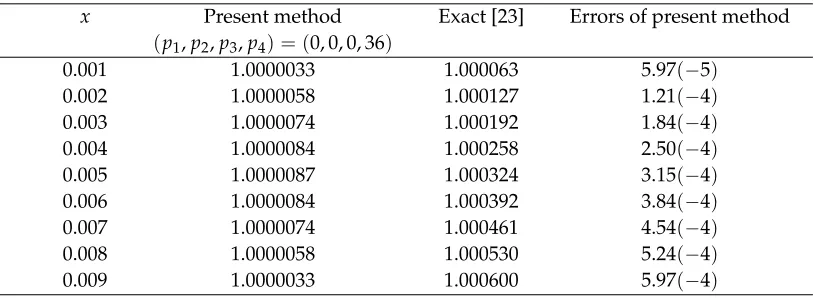
We have solved this example by scheme (2.20) and have obtained approximate solution atx=0.001(0.001)0.009 for the sake of comparison with references. The obtained numerical results are tabulated in table 1 and 2 for second and fourth order methods respectively. The comparison is also made in table 2 with the obatined results of [23].
Table 1. Maximum absolute errors for example 1
Second order method,ε=0.01,h=0.001
x Present method Exact [23] Errors of present method (p1,p2,p3,p4) = (0, 0, 0, 36)
0.001 1.0000033 1.000063 5.97(−5) 0.002 1.0000058 1.000127 1.21(−4) 0.003 1.0000074 1.000192 1.84(−4) 0.004 1.0000084 1.000258 2.50(−4) 0.005 1.0000087 1.000324 3.15(−4) 0.006 1.0000084 1.000392 3.84(−4) 0.007 1.0000074 1.000461 4.54(−4) 0.008 1.0000058 1.000530 5.24(−4) 0.009 1.0000033 1.000600 5.97(−4)
Conclusion
We have developed a numerical method for the solution of fourth order singularly pertubed boundary value problem using parametric septic spline. It is a computationally efficient method and the algorithm can easily be implemented on a computer. The method has been analysed for convergence and proved that the method is second and fourth order convergent. Also, the errors at nodal points are compared with the errors of [23] and observed to be better.
Table 2. Maximum absolute errors for example 1
Fourth order method,ε=0.01,h=0.001
x Present method Exact [23] Errors of present method Errors [23] (p1,p2,p3,p4) = (0, 0, 12, 12)
References
[1] A. H. Nayfeh,Introduction to Perturbation Methods, John Wiley and Sons, New York, (1981).
[2] B. Semper, Locking in finite element approximation of long thin extensible beams,IMA J. Numer. Anal., 14(1994), 97-109.
[3] E. C. Garland, Graded mesh difference schemes for singularly pertubed two point boundary value prob-lems,Math. Comput., 51(1988), 631-657.
[4] G. Akram and S. S. Siddiqi, End conditions for interpolatory septic splines, Int. J. Comput. Math., 12(82)(2005), 1525-1540.
[5] G. B. Loghmani and M. Ahmadinia, Numerical solution of singularly perturbed boundary value prob-lems based on optimal control strategy,Acta. Appl. Math., 112(2010), 69-78.
[6] G. Sun and M. Stynes, Finite element methods for singularly perturbed higher order elliptic two point boundary value problems I: Reaction diffusion type,IMA J. Numer. Anal., 15(1995), 117-139.
[7] G. Sun and M. Stynes, Finite element methods for singularly perturbed higher order elliptic two point boundary value problems II: Reaction diffusion type,IMA J. Numer. Anal., 15(1995), 117-139.
[8] H. G. Roos and M. Stynes, A uniformly convergent discretization method for a fourth order singular perturbation problem,Bonner Math. Schriften, 228 (1991), 30-40.
[9] H. G. Roos, M. Stynes and L. Tobiska,Numerical Methods for Singularly Perturbed Differential Equations, Springer, New York, (1996).
[10] J. Jayakumar and N. Ramanujam, A computational method for solving singular perturbation problems,
Appl. Math. Comput., 55(1993), 31-48.
[11] J. Jayakumar and N. Ramanujam, A numerical method for singular perturbation problems arising in chemical reactor theory,Comput. Math. Applic., 5(27)(1994), 83-99.
[12] K. Niederdrenk and H. Yserentant, The uniform stability of singularly perturbed discrete and continuous boundary value problems,Numer. Math., 41(1983), 223-253.
[13] M. Feckan, Singularly perturbed higher order boundary value problems, J. Differential Equations, 3(1)(1994), 79-102.
[14] M. K. Jain,Numerical Solution of Differential Equations, Wiley eastern Limited, New Delhi, India, (1979).
[15] M. K. Kadalbajoo and V. Gupta, A brief survey on numerical methods for solving singularly perturbed problems,Appl. Math. Comput., 217(2010), 3641-3716.
[16] M. K. Kadalbajoo and Y. N. Reddy, Numerical treatment of singularly perturbed two point boundary value problems,Appl. Math. Comput., 21(1987), 93-110.
[17] M. K. Kadalbajoo and Y. N. Reddy,Approximate methods for the numerical solution of singular perturbation problems, Appl. Math. Comput., 21 (1987) 85-199.
[18] P. Henrici,Discrete Variable Methods in Ordinary Differential Equations, Wiley, New York, (1962).
[19] R. K. Bawa, Spline based computational technique for linear singularly perturbed boundary value prob-lems,Appl. Math. Comput., 167(2005), 225-236.
[20] S. Natesan and N. Ramanujam, A computational method for solving singularly perturbed turning point problems exhibiting twin boundary layers,Appl. Math. Comput., 93(1998), 259-275.
[21] T. Aziz and A. Khan, A spline method for second order singularly perturbed boundary value problems,
[22] V. Shanthi and N. Ramanujam, A numerical method for boundary value problems for singularly per-turbed fourth order ordinary differential equations,Appl. Math. Comput., 129(2002), 269-294.
[23] V. Shanthi and N. Ramanujam, Asymptotic numerical methods for singularly perturbed fourth order ordinary differential equations of reaction diffussion type,Int. J. Comput. Math. Applic., 46(2003), 463-478.
[24] V. Shanthi and N. Ramanujam, A boundary value technique for boundary value problems for singularly perturbed fourth order ordinary differential equations,Comput. Math. Applics., 47(2004), 1673-1688.
[25] V. Shanthi and N. Ramanujam, Asymptotic numerical method for boundary value problems for sin-gularly perturbed fourth order ordinary differential equations with a weak interior layer,Appl. Math. Comput., 172(2006), 252-266.
Received: February 16, 2014;Accepted: November 7, 2014
UNIVERSITY PRESS