Score test in robust M-procedure

Journal of Applied Probability and Statistics 2001x, Vol. xx, No. xx, pp. xx-xx

Copyright ISOSS Publications 2014

SCORE TEST IN ROBUST M-PROCEDURE

Shahjahan Khan1

School of Agricultural, Computational and Environmental Sciences International Centre for Applied Climate Science

University of Southern Queensland, Toowoomba, Australia Email: [email protected]

Rossita M Yunus

Institute of Mathematical Sciences, Faculty of Sciences, University of Malaya, Kuala Lumpur, Malaysia.

Email: [email protected]

summary

A score type test based on the M-estimation method for a linear regression model is more reliable than the parametric based-test under mild departures from model assumptions, or when dataset has outliers. An R-function is developed for the score M-test, and applied to two real datasets to illustrate the procedure. The asymptotic power function of the M-test under a sequence of (contiguous) local alternatives is derived. Through computation of power function from simulated data, the M-test is compared with its alternatives, the Student’stand Wilcoxon’s rank tests. Graphical illustration of the asymptotic power of the M-test is pro-vided for randomly generated data from the normal, Laplace, Cauchy, and logistic distributions.

Keywords and phrases: Robust inference, M-test, Student’s t test, rank test, asymptotic power, and contiguity.

2010 Mathematics Subject Classification: Primary 62F03 & 62F35, and Secondary 62G10

1

Introduction

Robust statistical methods are essential to avoid any misleading or devastating impact on the inference due to the presence of any outliers, and/or violation of model assumptions. This approach is crucial when the traditional assumptions on the parametric inference are not satisfied or there are outliers in the sample dataset. The validity of any statistical inference depends on the appropriateness of the method applied. The commonly used Student’s

t test (introduced by Gosset, (1908)) is heavily dependent on the assumption of normal populations, and as such it is not valid for the data obtained from any other distributions. Moreover, the presence of outliers in the data makes the Student’sttest inappropriate.

Robust estimation methods are classified into three broad categories; M, L, and R-estimation (Huber, 1964). The M-R-estimation methods can be regarded as a generalization of maximum-likelihood estimation. The L-estimation methods are linear combinations of the ordered statistics, and the R-estimation methods are based on ranks of the observed data. Statistical tests were developed from/for the three categories of robust methods in the literature. For example, a signed rank test for a one sample location problem, a rank sum test for a two sample location problem (Wilcoxon, 1945), a rank test for linear models (H´ajek, 1962, Saleh and Sen, 1983) are among the popular tests that are based on ranks of the observed data. Using the M-estimation method, some robust tests were proposed in the literature. For example, Schrader and Hettmansperger (1980) proposed a test based on the likelihood ratio criterion, Fung et al. (1985) proposed a test that kept the form of the Student’st-test but used the score function in the M-estimation method to make their proposed test robust. Sen (1982) introduced a score M-test for linear models; and Yunus and Khan (2010, 2011a, 2011b) used the score M-test to investigate the effect of the pre-testing on the slope parameter on the final pre-testing of the intercept parameter of the linear regression models.

The nonparametric tests use the ranks of the observed data to formulate suitable test based on the rank sum statistics. In the process of ranking the observed data, valuable information, (details or magnitude) are lost, and is likely to impact on the quality of the test. For this reason the power of the nonparametric tests, in general, are lower than the equivalent parametric tests if the underlying distribution of the population is normal.

Any inference based on the M-procedure uses the original observed data values but treats the outliers to eliminate or minimize their impact on the inference using appropriate re-allocation of weights. As such, the M-procedure is less dependent on the assumptions of the population distribution. In the above sense, the M-test is robust. Although the exact distribution of the the M-test statistic is unavailable, its asymptotic distribution is used to workout the power function of the test. Since the M-statistic asymptotically follows a normal distribution its critical values are available from the normal table.

under the alternative hypotheses.

The derived asymptotic power functions of the score M-test are computed and graphically presented in this paper. Our paper provides the graphical analysis of the power function which was not the focus of many articles published earlier in this area (eg. Sen (1982) and Heritier and Ronchetti (1994)). The mathematical formula of power function is not reported in many articles in the area of robust statistical tests. Although the form of the power function of the score M-test is given in Sen (1982) and Jureˇckov´a and Sen (1996), the illustration of the power function through computation is unavailable. In our paper, the M-test for the one location and difference between two locations are implemented for real life data using newly defined R-functions. The associatedtand rank tests are also accompanied and compared with the M-tests. The power function of the M-test is presented graphically, and it is compared to that of the Student’stand Wilcoxon’s rank tests.

Since the M-test is not included in any popular statistical package, we provide the R-code and appropriate R-function to run the M-test for any given dataset for both one and two-sample cases. The R-function produces the observed value of the M-test statistic and the associated p-value. These values can be easily compared to the result of the relevant Student’stor relevant nonparametric test.

The two-sided M-test and its properties are given for one population and two populations in Section 2. Section 3 discusses the properties of the one-sided M-tests. Section 4 covers discussions on application of M-tests on two independent datasets. Section 5 illustrates the graphical comparisons of the power of the Student’s t, Wilcoxon’s rank and M-tests. The final Section provides discussions and concluding remarks. The R-codes and functions for the M-test are included in the Appendix.

2

The M-test

A linear regression model ofnobservable random variables,Yi, i= 1, . . . , nis given by

Yi =θ+βxi+ei, (2.1)

where thexi’s are known real constants of the explanatory variable with error termei, and θandβ are the unknown intercept and slope parameters respectively.

LetY1, Y2, . . . , Yn be identically and independently distributed random variables from a

continuous distribution function F(y) =Fi(yi−θ−βxi), yi, θ, β ∈ ℜ. Also, assume that F(yi−θ−βxi) is a symmetric (about zero) distribution function.

M-estimators forθ andβ are defined as the roots of the system of equations:

n

∑

i=1

ψ

(

Yi−θ−βxi Sn

)

= 0, (2.2)

n

∑

i=1

xiψ

(

Yi−θ−βxi Sn

)

where ψ is known as the score function in the M-estimation methodology. Here, Sn is an

appropriate scale statistic for some functional S = S(F) >0 and Sn is chosen to be the

median of the absolute deviations of the sample from its median.

The choice of a suitable robustψ-function justifies the test statistic. Severalψ-functions are available in the literature, among them the popular ones are the Huber’s, Hampel’s, and Tukey’sψ-functions.

• The Huber’s score function is defined as ψHuber(x) = x for |x| ≤ c, c sign(x) for

|x|> c, wherexis any real number andcis known as the tuning constant because it can be chosen to fine tune the estimator. The value of the tuning constant is chosen as 1.345 since this value produces a 95% efficiency relative to the mean sample (Holland and Welsch, 1977).

• The Hampel’s score function is written asψHampel(x) =x, for 0<|x| ≤a, asign(x),

for a≤ |x| ≤b, a(r− |x|)sign(x)/(r−b), forb ≤ |x| ≤r, 0 forr≤ |x|,where xis any real number anda,b andrare the tuning constants. The default values for these tuning constants used in R area= 2, b= 4 and r= 8.

• The Tukey’s score function is expressed asψT ukey(x) =x(1−(x/k)2)2 for |x| ≤k,

0 for x > k, wherexis any real number andkis a tuning constant. The value of the tuning constant is chosen as 4.685 since this value produces a 95% efficiency relative to the mean sample (Holland and Welsch, 1977).

In this paper, we consider three special cases of hypotheses testing in the linear regression model, (i) testing location of a population distribution, (ii) testing the equality of the loca-tions of two population distribuloca-tions and (iii) testing on the slope coefficient of a regression model.

2.1

The M-test for one location

Letβ = 0 in the equation (2.1), soθis the location of the distribution ofY. Assume that the distributionF(y−θ) is continuous. We wish to test the location of the distribution to be a specified value, that is,H0:θ=θ0 againstH0:θ̸=θ0.

An appropriate M-test, to testH0:θ=θ0againstHA:θ̸=θ0, is based on the following test statistic

M1n =M1n(θ0) =

n

∑

i=1

ψ

(

Yi−θ0

S1n

)

(2.4)

with scale statistic S1n. At the α-level of significance, the H0 is rejected if the observed value of the test statistic satisfies|M1n|> ℓ1n,α/2, whereℓ1n,α/2is the upperα/2-percentile of the distribution ofM1n.

symmetric about zero, then ∫ _∞

−∞

ψ

(

Yi−θ0

S1n

)

dF(Yi−θ0) = 0.

For large samples, underH0:θ=θ0,

n−12M_1n(θ₀)/S⋆

1n→N(0,1), (2.5)

whereS∗_1n2 =n−1∑n i=1ψ

2(Yi−θ˜

S1n

)

in which ˜θ is the studentized M-estimator of θbased on

Y1, Y2, . . . , Yn, and it is expressed as

˜

θ= 1 2sup

{

a:

n

∑

i=1

ψ((Yi−a)/S1n)>0

} +1

2inf {

a:

n

∑

i=1

ψ((Yi−a)/S1n)<0

}

,

andS₁∗_n2 →σ2

1 as n→ ∞, (cf. Jureˇckov´a and Sen, 1996, p. 409) and

σ2₁= ∫

ℜ

ψ2

(

Yi−θ S1

)

dF(Yi−θ), (0< σ1<∞)

is the second moment ofψ(·). If ψ(x) = x (i.e. the maximum likelihoodψ-function) and

F ∼N(0, σ2_{), thenS}

1=σandσ12= 1.

2.1.1 Properties of M1n

Letαbe the nominal significance level for the above test. Then the critical valueℓ1n,α/2 is such that

P(|M1n|> ℓ1n,α/2|H0) =P(M1n> ℓ1n,α/2, M1n<−ℓ1n,α/2|H0) =α. (2.6)

Let ϕ1n =I(|M1n|> ℓ1n,α/2) be the test function designated to test H0 : θ =θ0 against

HA:θ̸=θ0,whereI(A) is the indicator function of the setAwhich assumes values 0 or 1. Also, let Φ(x) be the standard normal distribution function of the random variableX and Φ(τα/2) = 1−α/2, 0< α <1. From equations (2.5) and (2.6), asn→ ∞,

n−12_ℓ

1n,α/2/S1∗n→τ1α/2. (2.7)

Now letα1n=E(ϕ1n|θ=θ0) be the size ofϕ1n. Then,

α1n=P(|M1n|> ℓ1n,α/2|H0:θ=θ0) =α

using equation (2.6). The power function of the test functionϕ1n,is defined as

Π1n(θ) = E(ϕ1n|θ) =P(|M1n|> ℓ1n,α/2|anyθ) = P[M1n> ℓ1n,α/2|anyθ

]

+P[M1n<−ℓ1n,α/2|any θ ]

Note that the size of the test α1n is a special case of the power function of the test when

the null hypothesis is true, i.e. α1n= Π1n(θ=θ0).

From the equation (5.5.29) of Jureˇckov´a and Sen (1996, p. 221), underH0, asngrows large,

sup {

n−12|M_1n(θ₀+a)−M_1n(θ₀) +nγ₁a|:|a| ≤n− 1 2K

}

→0, (2.9)

whereK is a positive constant, and

γ1= 1

S1 ∫

ℜ

ψ′

(

Yi−θ S1

)

dF(Yi−θ)

in whichψ′ is the derivative ofψ-function.

Further, consider a sequence of local alternative hypotheses {Hn}, where

Hn :θ=θ0+n−

1

2λ, λ >0.

Now utilizing the contiguity of probability measures (see H´ajek et al., 1999, Ch. 7) under

{Hn} to those under H0, equation (2.9) implies thatn−

1

2M_1n(θ₀) under {H_n} is

asymp-totically equivalent to n−12M_1n(θ₀+n− 1

2λ) +λγ₁. However, the asymptotic distribution

of n−12M_1n(θ₀) under {H_n} is the same as the distribution of n−12M_1n(θ₀−n−12λ) = n−12M_1n(θ₀) +λγ₁ underH₀, by the fact that the distribution ofM_1n(a) underθ=ais the

same as that ofn−12M_1n(θ−a) underθ= 0 (cf. Saleh, 2006, p. 332). Therefore, for a large

sample, under{Hn} the distribution of

n−12M_1n→N(λγ₁, σ2

1). (2.10)

Thus, under{Hn}, the asymptotic power function of the one-sample M-test is given by

Π1(λ) = lim

n_→∞Π1n= 1−Φ(τ1α/2−λγ1/σ1) + Φ(−τ1α/2−λγ1/σ1) (2.11)

using equations (2.8) and (2.10). Obviously, for any large sample size, the asymptotic size of the test for one-sample M-test is given by

α1= Π1(λ= 0) = 1−Φ(τ1α/2) + Φ(−τ1α/2) =α.

2.2

The M-test for difference of two locations

Let two independent random samples,U1, U2, . . . , Un1, and V1, V2, . . . , Vn2, be drawn from

the populations ofU andV such that,

P(Ui≤t) =P(Vj ≤t+β) =F(t), (2.12)

We want to test H₀∗: distribution ofU andV are identical againstH_A∗: V has different location thanU, and this is equivalent to testH₀∗:β = 0 againstH_A∗ :β̸= 0.

Let the two random samples fromU andV be merged to form a combined random sample

Y1, Y2, . . . , Yn, such thatY1=U1, Y2=U2, . . . , Yn1=Un1, Yn1+1=V1, . . . , Yn=Vn2,where n=n1+n2. Then the predictor variable in the equation (2.1)xk= 0,fork= 1,2, . . . , n1, andxk= 1,fork=n1+ 1, . . . , n.

Consider a M statistic,

M₂∗_n(˜θ,0) =

n2

∑

j=1

ψ

(

Vj−θ˜ S2n

) =

n

∑

k=1

xkψ

(

Yk−θ˜ S2n

)

, (2.13)

where ψis the score function and S2n is an appropriate scale statistic for some functional S2 =S2(F)>0. The median of the absolute deviations of the sampleY from its median is used as an estimate ofS2n. Note that ˜θis the constrained M-estimator ofθwhenβ = 0,

that is, ˜θis the solution of∑n_k=1ψ(Yk−a) = 0 and conveniently be expressed as

˜

θ = 1

2sup { a: n ∑ k=1 ψ (

Yk−a S2n

) >0 } +1 2inf { a: n ∑ k=1 ψ (

Yk−a S2n

)

<0 }

.

From Sen (1982) and Yunus and Khan (2011a), underH₀∗:β= 0,

M2n =

1

S₂∗_n√n1n2/n

n2

∑

j=1

ψ

(

Vj−θ˜ S2n

)

→N(0,1) asn→ ∞, (2.14)

whereS₂∗_n2 =n−1[∑n_k=1ψ2

(

Yk−θ˜

S2n

)] .

2.2.1 Properties of M2n

Consider a local sequence of alternative hypotheses{Kn}, where

Kn :β=n− 1

2η, η >0. (2.15)

Following similar steps as in the one-sample case, the asymptotic power function of the M-test for the two-sample problem under{Kn} is given by

Π2(η) = lim

n_→∞Π2n(β) = 1−Φ(τ2α/2−ηγ2

√

n1n2/nσ2) + Φ(−τ2α/2−ηγ2

√

n1n2/nσ2)(2.16)

using the asymptotic results of Jureˇckov´a and Sen (2006), and Yunus and Khan (2011a), where

γ2= 1 S2 ∫ ℜ ψ′ (

Yk−θ−βxk S2

)

dF(Yk−θ−βxk), (2.17)

in whichψ′ is the derivative of theψ-function and

σ₂2= ∫

ℜ

ψ2

(

Yk−θ−βxk S2

)

is the second moment ofψ(·).

The asymptotic size of the test is given by

α2= Π2(0) = 1−Φ(τ2α/2) + Φ(−τ2α/2) =α (2.19)

from equation (2.16).

2.3

The M-test for testing the slope coefficient

A convenient form of the M-test statistic for testing H0 : β =β0 against HA :β ̸=β0 for the model in (2.1) is given by

Mn=Mn⋆(˜θm, β0) =

n

∑

i=1

xiψ

(

Yi−θ˜m−β0xi Sn

)

say, (2.20)

where ˜θm is the constrained M-estimator of θ when β =β0, that is, ˜θm is the solution of M⋆

n(a, β0) = 0 and it may be conveniently be expressed as

˜

θ= [sup{a:M_n†(a, β0)>0}+ inf{a:Mn†(a, β0)<0}]÷2, (2.21)

whereM_n†(a, b) =∑n_i=1ψ

(

Yi−a−bxi

Sn

)

, aandbare any real numbers. ThenH0is rejected if

|Mn|> ℓn,α/2 at the αlevel of significance, whereℓn,α/2 is the upperα/2-percentile of the distribution ofMn.

It follows from the equation (2.6) of Yunus and Khan (2011a) that underH0,

n−12M_n→d N(0, σ2

0C

⋆2

) asn→ ∞, (2.22)

whereC⋆_{= lim}

n→∞

∑n i=1x

2

i −nx¯2n, x¯n=n−1

∑n

i=1xi, and σ2

0= ∫

ℜψ2

(

Yi−θ−βxi

S

)

dF(Yi−θ−βxi) (0< σ0<∞) is the second moment ofψ(·). Let

S_n⋆2=n−1 n

∑

i=1

ψ2

(

Yi−θ˜m−β0xi Sn

)

, (2.23)

(cf. Jureˇckov´a and Sen, 1996, p. 409) and S⋆ n

2_→

σ2

0 asn→ ∞.

2.4

Properties of

M

Now consider a sequence of local alternative hypotheses{Qn}, where

Qn:β=β0+n−

1

2_{ν, ν >0. (2.24)}

Using equations (2.22), and (5.5.29) of Jureˇckov´a and Sen (1996), and the contiguity

probability measures, under {Qn}, the distribution of n− 1

2M_n →d N(νγC⋆2, σ₀2C⋆2) (cf.

Following similar steps as in the one-sample case, the asymptotic power function of the M-test for testing the slope coefficient of the regression model under{Qn}, is given by

ΠM(ν) = 1−Φ(τα/2−νγC⋆σ0−1) + Φ(−τα/2−νγC⋆σ0−1), (2.25)

where

γ= 1

S

∫

ℜ

ψ′

(

Yi−θ−βxi S

)

dF(Yi−θ−βxi)

andψ′is the derivative ofψ-function. Hereτα/2 is the critical value of the standard normal distribution at theα/2 level of significance.

3

The one-sided tests

The adoption of the above two-sided M-test to a one-sided test is straightforward. Suppose we test H0 : β = 0 against HA : β > 0, then we work with M1n and the corresponding

critical valueℓ1n,αin (2.7), and obtain P(M1n > ℓ1n,α|H0) =α.It follows that the power function for a one-sided M-test for testing the location of one population is given by

Π1n(θ) =P[M1n> ℓn,α|anyθ]. (3.1)

As n → ∞, we find that the asymptotic power of a one-sided test for testing about the location of population is given by

Π1(λ) = lim

n_→∞Π1n(µ) = 1−Φ(τ1α−λγ1σ −1

1 ). (3.2)

In the same manner, the asymptotic power of a one-sided test for testing the equality of location parameter of two populations is given by

Π2(η) = 1−Φ(τ2α−ηγ2

√

n1n2/nσ2) (3.3)

and that for testing on the slope coefficient is given by

ΠM(ν) = 1−Φ(τα−νγC⋆σ−01). (3.4)

4

Applications on data

In this section, the R-codes to compute the value of the M-test statistic, its pvalue, confi-dence interval for θ and asymptotic power of the test are discussed. In the Appendix the R-function for the M-test is included. Users can choose to run a one-sided or two-sided test. The R-codes that produce the M-test statistic, p-value, confidence interval, σ1 and

functions for one-sample M-test are given in Listing 3. For the two-sample M-test, the R-codes that produce the M-test statistic and itsp-value, the asymptotic power and examples of using the M-test on data are given in Listings 4, 5, and 6. The formula and R-codes in this paper are based on the Tukey’sψ-function. The M-test for both one and two locations as well as its applications on two different datasets are included here.

4.1

One-sample M-test: Birth rate of 56 states in United States

in 2010

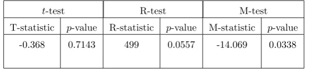
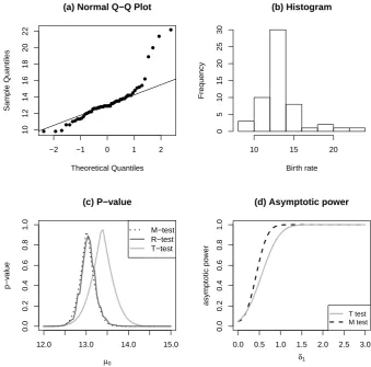
For the illustration of the M-test of one location we consider the birth rate dataset obtained from National Vital Statistics Report (Table 12. Birth rates, by age of mother: United States, each state and territory, 2010). Birth rate of 56 states in United States were measured for year 2010. The mean and median of birthrate is 13.38 and 12.6 respectively. It is observed from the normal Q-Q plot and the histogram given in Figures 1(a) and (b) that the distribution of the data is not normal. In facts, these figures reveal some outliers.

The observed value of the test statistic for thet-, R- and M-tests (Student’st, Wilcoxon’s rank and M-tests) along with thep-values are calculated for testingH0 :µ= 13.5 against

HA:µ̸= 13.5 at the 5% significance level and are given in Table 1. We find that thet-test

could not rejectH0 at the 5% significance level as the p-value is 0.7143. However, the R-and M-tests reject the null hypothesis as the p-values are 0.0557 and 0.0338, respectively (see Table 1). For this dataset, one may have a different null hypothesis, that is, to testµ

at a particular value, sayµ0, asµ0 can take any real number in this two-sided testing. We obtainp-value for each testing on the H0 :µ=µ0, and then we plot p-value against µ0 in Figure 1(c). We observed that the M-test is comparable in performance to the R-test, but not to thet-test. Figure 1(d) shows the asymptotic power curves of the M- andt-tests for the birth rate dataset. Obviously, asymptotic power of the M-test is higher than that of the

t test. Existing R-codes wilcox.test and t.test were used to find the statistics andp-values for the R- andt-tests, respectively, while coding for the M-test is given in the appendix.

Table 1: Test results for the birth rate data

t-test R-test M-test

T-statistic p-value R-statistic p-value M-statistic p-value

−2 −1 0 1 2

10

12

14

16

18

20

22

(a) Normal Q−Q Plot

Theoretical Quantiles

Sample Quantiles

(b) Histogram

Birth rate

Frequency

10 15 20

0

5

10

15

20

25

30

12.0 13.0 14.0 15.0

0.0

0.2

0.4

0.6

0.8

1.0

(c) P−value

µ0

p−v

alue

M−test R−test T−test

0.0 0.5 1.0 1.5 2.0 2.5 3.0

0.0

0.2

0.4

0.6

0.8

1.0

(d) Asymptotic power

δ1

asymptotic po

w

er

T test M test

Figure 1: Graphs of Q-Q plot and asymptotic power curves for birth rate dataset, where

δ1=|µ−µ0|.

Table 2: Test results for the iodine versus LOCM data

t-test R-test M-test

T-statistic p-value R-statistic p-value M-statistic p-value

−2 −1 0 1 2

20

40

60

80

100

120

Normal Q−Q plot of iodine dose

Theoretical Quantiles

Sample Quantiles

−2 −1 0 1 2

20

40

60

80

100

120

Normal Q−Q plot of LOCM dose

Theoretical Quantiles

Sample Quantiles

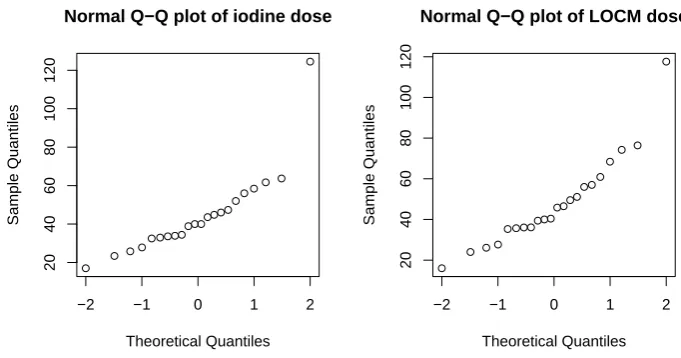
Figure 2: Graphs of Q-Q plot and histogram for iodine dose and LOCM dose.

4.2

Two-sample M-test: Iodine versus LOCM

A nephrotoxicity of iso-osmolar iodixanol is compared with a nonionic low-osmolar contrast media (LOCM) to find out which of them is more effective in reducing the risk of contrast media-induced nephropathy. In the study by Heinrich et al. (2009), serum creatinine levels are assessed before and after an intervascular application of iodixanol and LOCM.

The average of iodine and LOCM dose (mg/dL) are taken from 22 studies. We consider to testH₀∗: the distributions of iodine dose and LOCM dose are identical against H_A∗: the location of the distribution of iodine dose is different from the location of the distribution of LOCM dose. It is observed that there is one outlier in each normal Q-Q plot for the iodine dose and LOCM dose (see Figure 2). In the testing, we find H0∗ is not rejected at the 5% significance level using the t, rank and M-tests, respectively with p-values 0.5783, 0.4247 and 0.4425 (see Table 2).

5

Power Comparison

5.1

Test on the location of a population

ConsiderXi=µ+ei, i= 1,2, . . . , nwhereµis the location parameter andXi is a random

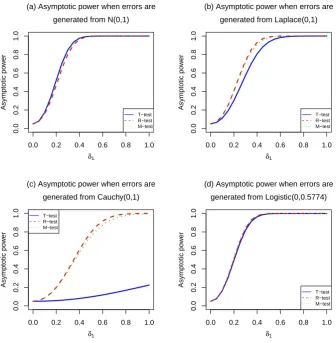
response with errorei. For the simulation, wet setµ= 2, α= 0.05,andn= 100.

Four symmetric distributions, namely the (i) normal, (ii) Laplace, (iii) Cauchy, and (iv) logistic, of error terms are considered to compare the asymptotic power of the tests. For the normal case, ei is generated from a normal distribution with mean 0 and variance

1. For the Laplace and Cauchy cases, ei is generated respectively from a Laplace and

Cauchy distribution with location 0 and scale 1, while for the logistic case,ei is from logistic

distribution with location 0 and scale 1/√3.

Asymptotic power of the M-test is computed using the function given in the equation (2.11) for the two-sided test. The estimate of γ1 in the equation (2.11) is taken as ˆγ1 =

1

n(M AD/0.6745) ∑n

i=1ψ′huber

(

Xi−µ˜

M AD/0.6745 )

, where M AD is the median absolute deviation

of the sample ofX. Theσ1 in the equation (2.11) is estimated byS1∗n usingψ=ψhuber.

The simulation is run 10,000 times to get 10,000 simulated sets of values of error terms. Using Xi = 2 +ei, i = 1,2, . . . , n, we obtain 10,000 simulated datasets of size n = 100.

Then, these datasets are used to computeS₁∗_n and ˆγ1. The average of asymptotic power of the test for the 10,000 simulated datasets is computed at a particular value ofδ1=|µ−µ0|. After 10,000 repetitions, the value ofδ1was increased and the process repeated. The curves of the asymptotic power of the tests for increasing values ofδ1 are plotted in Figure 3.

It is depicted in Figure 3(a) that asymptotic power of the M-test is as much as that of thet-test, and power of both tests are slightly higher than that of the R-test when data is generated from normal distribution. However, the asymptotic power of the R- and M-tests is larger than that of thet-test when sample data is generated from the Laplace and Cauchy distributions ((b) and (c)). It is observed that M-test is comparable in terms of power to the R-test when the distribution of data is Cauchy (heavy tails) or Laplace (light tails). All the tests have similar power when sample data is generated from logistic distribution ((d)).

5.2

Test on the equality of location of two populations

Consider two independent random samples, U1, U2, . . . , Un1 and V1, V2, . . . , Vn2, from the

random variablesU andV, where the two distributions are identical except for the difference in the location. Let β be the difference between the two locations of the two populations. In the simulation study, we setα= 0.05 andn1=n2= 100,so n=n1+n2= 200.

Four distributions, namely the (i) normal, (ii) Laplace, (iii) Cauchy, and (iv) logistic, of

U and V are considered to compute the asymptotic power function of the M-test. For the normal case,U is generated from a normal distribution with location/mean 2 and variance 1 and V is generated from a normal distribution with location/mean 2 +β and variance 1. For the Laplace, Cauchy and logistic cases, U is generated respectively from a Laplace, Cauchy or logistic distribution with a location parameter 2 and a scale parameter 1 and

0.0 0.2 0.4 0.6 0.8 1.0

0.0

0.2

0.4

0.6

0.8

1.0

δ1

Asymptotic po

w

er

(a) Asymptotic power when errors are

generated from N(0,1)

T−test R−test M−test

0.0 0.2 0.4 0.6 0.8 1.0

0.0

0.2

0.4

0.6

0.8

1.0

δ1

Asymptotic po

w

er

(b) Asymptotic power when errors are

generated from Laplace(0,1)

T−test R−test M−test

0.0 0.2 0.4 0.6 0.8 1.0

0.0

0.2

0.4

0.6

0.8

1.0

δ1

Asymptotic po

w

er

(c) Asymptotic power when errors are

generated from Cauchy(0,1)

T−test R−test M−test

0.0 0.2 0.4 0.6 0.8 1.0

0.0

0.2

0.4

0.6

0.8

1.0

δ1

Asymptotic po

w

er

(d) Asymptotic power when errors are

generated from Logistic(0,0.5774)

T−test R−test M−test

0.0 0.2 0.4 0.6 0.8 1.0

0.0

0.2

0.4

0.6

0.8

1.0

δ2

Asymptotic po

w

er

Student’s t test Hampel’s M test Huber’s M test Tukey’s M test

(a) Asymptotic power when samples

from normal distribution

0.0 0.2 0.4 0.6 0.8 1.0

0.0

0.2

0.4

0.6

0.8

1.0

δ2

Asymptotic po

w

er

Student’s t test Hampel’s M test Huber’s M test Tukey’s M test

(b) Asymptotic power when samples

from Laplace distribution

0.0 0.2 0.4 0.6 0.8 1.0

0.0

0.2

0.4

0.6

0.8

1.0

δ2

Asymptotic po

w

er

Student’s t test Hampel’s M test Huber’s M test Tukey’s M test

(c) Asymptotic power when samples

from Cauchy distribution

0.0 0.2 0.4 0.6 0.8 1.0

0.0

0.2

0.4

0.6

0.8

1.0

δ2

Asymptotic po

w

er

Student’s t test Hampel’s M test Huber’s M test Tukey’s M test

(d) Asymptotic power when samples

from logistic distribution

identical distribution ifβ = 0.

Asymptotic power of the two-sided M-test is computed using the form of asymptotic power function given in equation (2.16). The estimate ofγ2in the equation (3.3) is taken as

1

n M AD/0.6745 ∑n

k=1ψ′ (

Yk−θˆm−βˆmck

M AD/0.6745 )

andσ2 is estimated by √

1

n

∑n k=1ψ2

(

Yk−θˆm−βˆmck

M AD/0.6745 )

,

where ˆθmand ˆβmare the M-estimates for parametersθandβof the simple regression model

in (2.10), andM ADis the median absolute deviation of the sample ofY. In the simulation, the Hampel’s, Huber’s, and Tukey’s ψ-functions are considered to obtain the asymptotic power of the M-test.

The simulation is run 10,000 times to get 10,000 simulated sets of values of both samples datasets. Then, these datasets are used to compute S₂∗_n, and ˆγ2. After 10,000 repetitions, the value of theδ2 was increased and the process repeated. The asymptotic power curves for increasing values ofδ2 were plotted in Figure 4.

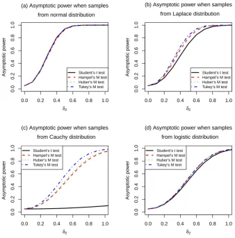
From Figure 4, we find that the M-test based on the Hampel’s, Huber’s, and Tukey’s

ψ-functions are more robust against departures from the normal distribution assumption as their powers are larger than that of the Student’st-test. The power of M-test based on the Hampel’sψ-function are close to that of the Student’st-test when sampling is done from the normal distribution. The M-test based on the Huber’s and Tukey’s ψ-functions have larger power than that of the Hampel’s when the samples are from the Laplace and Cauchy distributions.

6

Concluding remarks

The use of M-test removes any chance of misleading test outcome due to the violation of assumptions or existence of outliers. Furthermore, the asymptotic power of the M-test is at least as large as that of the Student’stor relevant nonparametric test when the assumptions are not met and even if there are no outliers. Clearly for the users it is advantageous to use the M-test to avoid any risk of using a test whose underlying assumptions may have been violated and hence the validity of the test outcomes becomes untenable.

In many cases the ordinary users of statistical tests do not bother to check the validity of the assumptions. For those users M-test is a better option as it provides much needed protection against the adverse consequences of the presence of outliers or departure from the assumptions on the population distribution.

6.1

Acknowledgements

References

[1] Fung K.Y., Lee H. and Tajuddin, I. (1985). Some Robust Test Statistics for the Two-Sample Location Problem.Journal of the Royal Statistical Society Series D (The Statis-tician),34, 2, 175-182.

[2] Gagliardini, P., Trojani, F. and Urga, G. (2005). Robust GMM tests for structural breaks.Journal of Econometrics,129, 139-182.

[3] Gosset, W.S. (1908). The probable error of a mean.Biometrika,6,125.

[4] H´ajek, J. (1962). Asymptotically Most Powerful Rank-Order Tests. Ann. Math. Statist., 33, 3 , 1124-1147.

[5] H´ajek, J., ˇSid´ak, Z. and Sen, P.K. (1999). Theory of Rank Tests. Academia Press, New York.

[6] Heritier, S. and Ronchetti, E. (1994), Robust bounded-influence tests in general para-metric models.J. Amer. Statist. Assoc.,89, 897-904.

[7] Holland, P.W. and Welsch, R.E. (1977). Robust regression using iteratively reweighted least-squares.Communications in Statistics - Theory and Methods, A,6, 813-838. [8] Huber, P.J. (1964). Robust estimator of a location parameter.Ann. Math. Statist.,35,

1, 73-101.

[9] Jureˇckov´a, J. and Sen, P.K. (1996). Robust Statistical Procedures Asymptotics and Interrelations. Wiley, New York.

[10] Markatou, M. and Hettmansperger, T. P. (1990), Robust bounded-influence tests in linear models.J. Amer. Statist. Assoc.,85, 187-190.

[11] Markatou M. He. X (1994) Bounded influence and high breakdown point testing pro-cedures in linear models.J. Amer. Statist. Assoc.,89, 42, 543-549.

[12] Muller, C. (1998). Optimum robust testing in linear models.Ann. Statist., 26, 1126-1146.

[13] Saleh, A.K.Md.E. (2006). Theory of Preliminary test and Stein-type estimation with applications. Wiley, New Jersey.

[14] Saleh, A.K.Md.E. and Sen, P.K. (1983). Nonparametric tests of location after a prelim-inary test on regression in the multivariate case.Communications in Statistics: Theory and Methods,12, 1855-1872.

[15] Schrader, R.M. and Hettmansperger, T.P. (1980). Robust analysis of variance based upon a likelihood ratio criterion.Biometrika,67, 1, 93-101.

[16] Sen, P.K. (1982). On M tests in linear models.Biometrika,69, 245-248.

[18] Silvapulle M.J and Silvapulle P. (1995). A Score Test Against One-Sided Alternatives. J. Amer. Statist. Assoc.,90, 429, 342 - 349.

[19] Sinha S. and Wiens D.P. (2002) Minimax Weights for Generalised M-Estimation in Biased Regression Models.The Canadian Journal of Statistics / La Revue Canadienne de Statistique,30, 3, 401-414.

[20] Wilcoxon, F. (1945). Individual comparisons by ranking methods.Biometrics Bulletin, 1, 6, 80-83.

[21] Yunus, R.M. and Khan, S. (2010). Increasing power of robust test through pre-testing in multiple regression model. Pakistan Journal of Statistics, Special Volume on 25th Anniversary, (Edited by S.E. Ahmed)26, 151-170.

[22] Yunus, R.M. and Khan, S. (2011a). Increasing the power of the test through pretest -a robust method.Communications in Statistics-Theory and Methods,40, 581-597. [23] Yunus, R.M. and Khan, S. (2011b). M tests for multivariate regression model.Journal

of Nonparametric Statistics,23, 201-218. R-Codes

(i) M-test for testing the location of a population

m.test1<-function(X, alternative = c("two.sided", "less", "greater"), mu.not, sig.level){

n<-length(X) library(MASS) mad.X<-mad(X) fit<-rlm(X~1)

r1<-(X-mu.not)/mad.X r2<-(X-fit$coef)/mad.X

Mstat<-sum(psi.huber(r1,deriv=0)*r1)

sigma <-sqrt((1/n)*sum((psi.huber(r2,deriv=0)*r2)^2)) gamma <-(1/n)*(sum(psi.huber(r2, deriv = 1)))/mad.X standardized.Mstat<-Mstat/(sigma*sqrt(n))

if (alternative =="greater") {

p.value<-1-pnorm(standardized.Mstat) }

if (alternative =="less") {

p.value <-pnorm(standardized.Mstat) }

if (alternative =="two.sided"){ p.value <-if (standardized.Mstat>=0)

2*pnorm(standardized.Mstat) }

interval <-c(fit$coef-(qnorm(1-sig.level/2))*sqrt(1/n)*mad.X, fit$coef+(qnorm(1-sig.level/2))*sqrt(1/n)*mad.X) list(Mstat=Mstat, standardized.Mstat=standardized.Mstat, p.value=p.value,M.estimate = fit$coef, interval=interval, sigma=sigma, gamma=gamma)

} }

(ii) The asymptotic power of the M-test for testing the location of one population

power.m.test1<-function(n, alternative=c("one.sided","two.sided"),delta, sigma, gamma, sig.level){

lambda<-delta*sqrt(n)

if (alternative =="one.sided"){

power<-1-pnorm(qnorm(1-sig.level)- lambda*gamma/sigma)} if (alternative =="two.sided"){

power<-1-pnorm(qnorm(1-sig.level/2)- lambda*gamma/sigma)+pnorm(-qnorm(1-sig.level/2)- lambda*gamma/sigma)}

list(power=power) }

(iii) Examples

X = c(12.6, 16.2, 13.7, 13.2, 13.7, 13.2, 10.6, 12.7, 15.2, 11.4, 13.8, 14.0, 14.8, 12.9, 12.9, 12.7, 14.2, 12.9 ,13.8, 9.8, 12.8, 11.1, 11.6, 12.9, 13.5, 12.8, 12.2, 14.2, 13.3, 9.8, 12.2, 13.5, 12.6, 12.8, 13.5, 12.1, 14.2, 11.9, 11.3, 10.6, 12.6 ,14.5, 12.5, 15.4, 18.9, 9.9, 12.9, 12.9, 11.0, 12.0, 13.4, 11.3, 15.1, 21.4, 22.2, 20.0)

fit1<-m.test1(X, alternative = "two.sided", mu.not=13.5, sig.level=0.05) power.m.test1(length(X),alternative="two.sided",delta=1 ,fit1$sigma, fit1$gamma,0.05)

(iv) M-test for testing the equality of location of two populations

m.test2<-function(X, Y, alternative = c("two.sided", "less", "greater"), psi.function =c("psi.huber", "psi.bisquare", "psi.hampel"),sig.level){

n1<-length(X) n2<-length(Y) n<-n1+n2 Z<-c(X,Y)

ci<-c(rep(0,n1),rep(1,n2)) vec.unit<-rep(1,n)

if(psi.function =="psi.huber") {

fit.full<-rlm(matrix(c(vec.unit,ci),ncol=2),Z)

psi.full<-psi.huber(fit.full$res/mad(fit.full$res),deriv=0)* (fit.full$res/mad(fit.full$res))

sigma.full<-sqrt(sum(psi.full*psi.full)/n) fit.null<-rlm(Z~1) #fit.null$s !=mad(Z)

psi.null<-psi.huber((Z-fit.null$coef)/mad(Z),deriv=0)* ((Z-fit.null$coef)/mad(Z))

sigma.null<-sqrt(sum(psi.null*psi.null)/n)

gamma <-(1/n)*(sum(psi.huber(fit.full$res/mad(fit.full$res), deriv = 1)))/mad(fit.full$res)

}

if(psi.function =="psi.bisquare") {

fit.full<-rlm(matrix(c(vec.unit,ci),ncol=2),Z, psi=psi.bisquare) psi.full<-psi.bisquare(fit.full$res/mad(fit.full$res),deriv=0)*

(fit.full$res/mad(fit.full$res)) sigma.full<-sqrt(sum(psi.full*psi.full)/n) fit.null<-rlm(Z~1, psi=psi.bisquare)

psi.null<-psi.bisquare((Z-fit.null$coef)/mad(Z),deriv=0)* ((Z-fit.null$coef)/mad(Z))

sigma.null<-sqrt(sum(psi.null*psi.null)/n)

gamma <-(1/n)*(sum(psi.bisquare(fit.full$res/mad(fit.full$res), deriv = 1)))/mad(fit.full$res)

}

if(psi.function =="psi.hampel") {

fit.full<-rlm(matrix(c(vec.unit,ci),ncol=2),Z, psi=psi.hampel) psi.full<-psi.hampel(fit.full$res/mad(fit.full$res),deriv=0)*

(fit.full$res/mad(fit.full$res)) sigma.full<-sqrt(sum(psi.full*psi.full)/n) fit.null<-rlm(Z~1, psi=psi.hampel)

((Z-fit.null$coef)/mad(Z)) sigma.null<-sqrt(sum(psi.null*psi.null)/n)

gamma <-(1/n)*(sum(psi.hampel(fit.full$res/mad(fit.full$res), deriv = 1)))/mad(fit.full$res)

}

M.stat <-sum(ci*psi.null)/sqrt(n*(sigma.null^2)*n1*n2/(n^2)) if (alternative =="greater")

{

p.value<-1-pnorm(M.stat) }

if (alternative =="less") {

p.value <-pnorm(M.stat) }

if (alternative =="two.sided") {

p.value <-if (M.stat>=0) 2*(1-pnorm(M.stat)) else 2*pnorm(M.stat) }

list(Mstat=M.stat, p.value=p.value, sigma=sigma.full, gamma=gamma) }

(v) The asymptotic power of the M-test for testing location of two populations

power.m.test2<-function(n1, n, alternative=c("one.sided","two.sided"), delta, sigma, gamma, sig.level){

lambda<-delta*sqrt(n)

if (alternative =="one.sided"){

power

<-1-pnorm(qnorm(1-sig.level)-sqrt(n1*(n-n1)/(n^2))*lambda*gamma/sigma)} if (alternative =="two.sided"){

power<-1-pnorm(qnorm(1-sig.level/2)-sqrt(n1*(n-n1)/(n^2))*lambda* gamma/sigma)+pnorm(-qnorm(1-sig.level/2)-sqrt(n1*(n-n1)/(n^2))* lambda*gamma/sigma)}

list(power=power) }

(vi) Examples

locm.dose<-c(39.4, 40, 56, 49.5, 51.1, 117.6, 40.4, 36.1, 57, 16, 45.84, 24, 35.7, 27.65, 74.22, 46.5, 26.1, 35.3, 68.4, 36.05, 76.4, 60.9) X<-iodi.dose

Y<-locm.dose delta<- 2 n1<-length(X) n<-length(c(X,Y))

fit2<-m.test2(X, Y, alternative = "two.sided", 0.05)