Why Welch’s test is Type I error robust.
Ben Derrick
a, Deirdre Toher
a& Paul White
a,aUniversity of the West of England, Bristol, England
Abstract The comparison of two means is one of the most commonly applied statistical procedures in psychology. The independent samples t-test corrected for unequal variances is commonly known as Welch’s test, and is widely considered to be a robust alternative to the independent samples t-test. The properties of Welch’s test that make it Type I error robust are examined. The degrees of freedom used in Welch’s test are a random variable, the distributions of which are examined using simulation. It is shown how the distribution for the degrees of freedom is dependent on the sample sizes and the variances of the samples. The impact of sample variances on the degrees of freedom, the resultant critical value and the test statistic is considered, and hence gives an insight into why Welch’s test is Type I error robust under normality.
Keywords Independent samples t-test; Welch’s test; Welch’s approximation; Behrens-Fisher problem; Equality of means.
Introduction
One of the most commonly applied hypothesis test proce-dures in applied research is the comparison of two popu-lation means (Wilcox,1992). For theoretical development purposes, assume two normally distributed populations N(µ1,σ21) andN(µ2,σ22) are to be compared based uponn1 andn2mutually independent observations. LetXiandS2i
denote random variables for sample means and variances respectively (i=1, 2).1If the population variances,σ21and σ2
2, are assumed to be equal, then an appropriate test statis-tic is the independent samples t-test, based on (1) and (2).
T1=
X1−X2 StandardError(X1−X2)
(1)
In the independent samples t-test, the standard error of (X1−X2), saySE1, is given by:
SE1=Sp r
2 ˜
n (2)
whereSp= r
(n1−1)S12+(n2−1)S22
(n1−1)+(n2−1) and ˜nis the harmonic mean
ofn1andn2.T1is referenced against the t-distribution with degrees of freedom equal toυ1=n1+n2−2.
It is known that, when the assumptions of the indepen-dent samples test are met, the indepenindepen-dent samples t-test is an exact t-test and is the most uniformly powerful t-test (Sawilowsky & Blair,1992). The independent samples t-test is an approximate test when population variances are equal. If sample sizes are unequal and variances are un-equal, the probability of rejecting the null hypothesis when
it is true deviates from the nominal Type I error rate. This is particularly problematic when the smaller sample size is associated with the larger variance (Zimmerman & Zumbo, 2009; Coombs, Algina, & Oltman,1996). This gives rise to the dilemma of how to compare means in the presence of unequal variances. This question, applied to two indepen-dent random samples from normal populations, is known as the Behrens-Fisher problem. Behrens (1929) and Fisher (1935,1941) suggested a solution for the problem. It is pro-posed that the t-test when equal variances cannot be as-sumed is defined as per (3) and (4).
T2=
X1−X2
StandardError(X1−X2) (3)
In the unequal variances case, the standard error of (X1− X2), saySE2is estimated by:
SE2= s
S2 1 n1+
S2 2 n2
(4)
The formula developed for the degrees of freedom is com-plex, but it is proposed that an approximation for the de-grees of freedom could be given by (5). This is given in most textbooks (e. g., Alfassi, Boger, & Ronen,2005; Miles & Ban-yard,2007).
υ2=
µ S21 n1+
S22 n2
¶2
µ S21 n1
¶2
/ (n1−1)+ µ
S22 n2
¶2
/ (n2−1)
(5)
1As standard notation, random variables are shown in upper case, and derived sample values are shown are in lower case.
TheQuantitativeMethods forPsychology 30
A numerically equivalent expression for the approxima-tionυ2is given in (6). This is shown in some textbooks (e. g., Ott & Longnecker,2001).
υ2= (n1−1)(n2−1)
(n2−1)c2+(n1−1) (1−c)2
(6)
where
c= S 2 1/n1
S2 1
n1+
S2 2
n2
The approximation υ2 dates back to a series of pa-pers by Welch (1938, 1947, 1951), independent work by Satterthwaite (1946), works by Fairfield-Smith (1936), and Aspin (1948,1949). The independent samples t-test cor-rected for unequal variances is sometimes referred to as the Satterthwaite-Smith-Welch test, the Welch-Aspin-Satterthwaite test, or other interchangeable variations. This may be referred to generically as the unequal vari-ances t-test, or as the separate varivari-ances t-test. Usually the unequal variances t-test with the degrees of freedom ap-proximated as above is simply known as Welch’s test.
Originally, an alternative approximation for the degrees of freedom given by Welch, is given in (7):
υ3=
µ S2
1
n1+
S2 2 n2 ¶2 µ S2 1 n1 ¶2
/ (n1+1)+ µ
S2 2
n2
¶2
/ (n2+1)
−2 (7)
The approximation is given in some textbooks (e. g. Frank & Althoen,1994), rounded down to the nearest integer. How-ever,υ3is not generally used, and is not numerically equiv-alent toυ2.
Textbooks frequently recommend the calculation ofυ2, rounded down to the nearest integer (e. g. Frank & Althoen, 1994; Ott & Longnecker,2001). Rounding down tends to produce a conservative test. More generally, some text-books recommend rounding to the nearest integer (e. g. Al-fassi et al., 2005). The rounding requirements appear in textbooks for the purposes of manual calculations. There is a need to use integer degrees of freedom when using sta-tistical tables for critical values. However, the calculation of Welch’s test is easy in statistical software such as R and SPSS (Rasch, Kubinger, & Yanagida,2011). These statisti-cal software would ordinarily conduct the test with non-integer degrees of freedom.
Welch’s test better approximates nominal significance levels, and has greater power than the Behrens-Fisher so-lution (Lee & Gurland,1975; Best & Rayner,1987). Fay and Proschan (2010, p. 14) confirm that Welch’s solution “is ap-proximately valid for the Behrens-Fisher perspective”.
When sample sizes are equal and variances are equal, both the independent samples t-test and Welch’s test perform similarly (Zimmerman & Zumbo, 1993; Moser, Stevens, & Watts,1989). For unequal sample sizes and un-equal variances, Welch’s test has superior Type I error ro-bustness (Fagerland & Sandvik,2009). Ruxton (2006) advo-cates the routine use of Welch’s test.
Grimes and Federer (1982, p.10) state that, "In the case of comparing two sample means, the consensus in the lit-erature seems to be the approval of Welch’s approximate solution". Thus the most commonly used solution to the Behrens-Fisher problem, is Welch’s test with the degrees of freedom calculated by approximation. In a practical envi-ronment, Welch’s approximation can be used with little loss of accuracy (Wang,1971; Scheffe,1970).
It can be seen from (5) that Welch’s degrees of freedom, υ2, is a random variable and therefore has its own sampling distribution. Consequently the critical value used in hy-pothesis testing is also a random variable. In addition, it can be seen from (4) that the sample variances affect both the value of T2and the value ofυ2.
In this paper; worked examples of the independent samples t-test and Welch’s test are provided. The distribu-tions of the degrees of freedom for Welch’s test are explored, and the two methods of estimating the standard error of are considered. Simulation is used to identify how the esti-mated standard error facilitates the Type I error robustness of Welch’s test, and provides insight into why the Welch test works in a practical environment.
Worked examples
As part of an investigation into sensitivity when exposed to evidence of "White Privilege", Phillips and Lowery (2015) randomly allocated U.S. participants who self-identified as White/European-American into two groups. The partici-pants completed a survey about equality and their child-hood memories ("Experiment 1a"). Prior to completing the survey, Group 1 (n1=54) were given a paragraph to read about "White Privilege", whereas Group 2 (n2=40) were not. Questions on the survey measured participants per-ceived "life hardship" on a Likert type scale, between 1 = "strongly disagree" and 7 = "strongly agree". The authors performed the independent samples t-test using each par-ticipant’s mean score.2 This implies that equality of vari-ance between groups is assumed; this is a seemingly rea-sonable assumption due to the random assignment of par-ticipants. For demonstration purposes, both the indepen-dent samples t-test and Welch’s test are provided in the present paper. For "Experiment 1a", the published data are as follows; the average participant score for Group 1 is 4.41, (standard deviation of 1.20). The average participant
2The published results differ slightly from the calculations given here, due to the use of the published (rounded) sample data in the present paper.
TheQuantitativeMethods forPsychology 31
score for Group 2 is 3.82 (standard deviation of 1.20). Thus, x1=4.410, s2
1=1.440, x2=3.820 ands22=1.440. Calcula-tions for the independent samples t-test give: sp =1.200,
se1=0.250,t1=2.357,υ1=92.000, the p-value using the in-dependent samples t-test is 0.021. Calculations for Welch’s test give:se2=0.250,t2=2.357,υ2=84.186, the p-value us-ing Welch’s test is 0.021. It can be seen that because the two sample variances are equal,t1=t2. The degrees of freedom applicable for each test are different, but the impact of this on the critical values of the tests is small. Thus the p-values for both tests are the same to three decimal places. The sta-tistical conclusion made at the 5% significance level, is that the sample mean for Group 1 is significantly greater than the sample mean for Group 2. The authors conclude that perceived "life hardship" is greater when participants are subjected to evidence of "White Privilege".
Phillips and Lowery (2015) replicated this experiment withn1=49 andn2=42 participants ("Experiment 1b"). The published data shows that the average participant score for Group 1 is 4.53, (standard deviation of 1.52). The average participant score for Group 2 is 3.96, (standard de-viation of 1.28). Thus, x1=4.530, s21=2.310, x2=3.960 ands22=1.638. Calculations for the independent samples t-test give: sp=1.415,se1=0.297,t1=1.916,υ1=89.000, the p-value using the independent samples t-test is 0.059. Calculations for Welch’s test give: se2=0.294, t2=1.942, υ2=88.978, the p-value using Welch’s test is 0.055. In this experiment, the p-values for the two tests are different due to the unequal sample sizes and unequal variances of the two samples. With reference to Experiment 1b, the authors state that participants in Group 1 claim more "life hard-ship" than participants in Group 2. However, for either test, at the 5% significance level, Experiment 1b alone rep-resents insufficient statistical evidence that there is a differ-ence between Group 1 and Group 2.
Methodology
Simulation is used to investigate Welch’s test for Type I er-ror robustness, and the distributional properties ofυ2. For both the independent samples t-test and Welch’s test, two sided tests are performed with nominal Type I error rate of α=0.05. The aim is to demonstrate deviations from Type I error robustness for the independent samples t-test for unequal variances. The standard error of the indepen-dent samples t-test and Welch’s test are explored to assess the impact of the standard error on the result of the tests. To achieve these goals, simulations underH0for two nor-mally distributed samples are performed as per the layout in Table1; withn1at two levels, n2at two levels andσ2 at two levels. Parameters are selected to cover both "large" and "small" samples and equal and unequal variances. The sample sizes represent extreme scenarios in order to assist
in the illustration of the effects.
For each scenario in the simulation design, 10,000 iter-ations are performed under the condition whereH0is true.
Results
Welch’s degrees of freedom.
The investigation of the distribution ofυ2, gives insight into when the degrees of freedom used in Welch’s test differ from the degrees of freedom used in the independent sam-ples t-test.
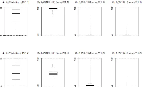
Figure1shows the distribution of the degrees of free-dom for each of the 8 scenarios simulated (10,000 observa-tions per scenario).
Inspection of Figure1shows the greatest discrepancy betweenυ1andυ2to occur whenn16=n2. The simula-tions demonstrate that [mi n{n1,n2}−1]≤υ2≤υ1. This
can be proven mathematically using (6). By differentia-tion, the maximum value ofυ2is found whens21/s22={(n1− 1)n1}/{(n2−1)n2}. The minimum value ofυ2is fixed by the sample with the larger variance. If Sample 1 has the larger variance, then the lower bound isn1−1. If Sample 2 has the larger variance, then the lower bound isn2−1. Hence, mi n{n1,n2}−1 is a very conservative approximation to the degrees of freedom when the smaller sample size is associ-ated with the larger variance. To illustrate these points, see Figure2with a fixed variance for Sample 1.
From Figure 2 it can be seen that as s22/s21 tends to zero, the degrees of freedom tends ton1−1. Ass22/s12 be-comes increasingly large, the degrees of freedom asymp-totically tends ton2−1. The maximum value occurs when s2
1/s22={(n1−1)n1}/{(n2−1)n2}. The examples have a total sample size of 30, thus the maximum value ofυ2is 28.
Type I error robustness for the independent samples t-test and Welch’s test.
In this section, p-values calculated from performing both the independent samples t-test and Welch’s test are con-sidered, as per the simulation design in Table1. IfH0is true and if underlying assumptions hold, then the p-values from a valid test procedure are expected to be uniformly distributed (Bland,2013). Deviations from uniformity give evidence that the test is not Type I error robust. If p-values are consistently less than expected under a uniform distri-bution, the test gives too many false positives, and is said to be “liberal”. If p-values are consistently greater than ex-pected under a uniform distribution, the test is “conserva-tive”.
There is negligible difference between the p-values when performing the independent samples t-test or Welch’s test under equal variances, regardless of sample size. In this case, p-values are approximately uniformly
dis-TheQuantitativeMethods forPsychology 32
Table 1 Summary of the simulation design.
Test statistics T1,T2 Degrees of freedom υ1,υ2
Sample sizes (n1,n2) (5,5), (5,100), (100,5), (100,100) Standard deviations (σ1,σ2) (1,1), (1,2)
Programming language R version 3.1.2 (R Development Core Team,2013)
tributed for both tests (results not shown).
When variances are unequal, Welch’s test is not a lin-ear function of the independent samples t-test. Figure3 is a P-P plot (percentile-percentile plot), for p-values for both the independent samples t-test (T1) and Welch’s test (T2), with unequal variances. This shows ordered expected p-values from a uniform distribution plotted against or-dered observed p-values. Given that for a valid test pro-cedure, observed p-values should be approximately uni-formly distributed on (0, 1) then an approximate diagonal would demonstrate Type I error robustness.
Both panels of Figure3show that when sample sizes are unequal and variances are unequal, the independent ples t-test is not Type I error robust. When the smaller sam-ple size is associated with the larger variance (left panel, Figure 3), the observed p-values under the independent samples t-test are smaller than expected, and the test is lib-eral. Conversely, when the larger sample size is associated with the larger variance (right panel, Figure3), the p-values are larger than expected and the independent samples t-test is conservative, (i.e. the expected Type I error rate is less than the pre-chosen nominal level of significance,α).
The p-values for Welch’s test are also given in Figure3. The simulated p-values for Welch’s test, are approximately uniformly distributed. This results in the approximate line of equality observed. Welch’s test therefore "corrects" for the fact that the independent samples t-test gives p-values that are not Type I error robust.
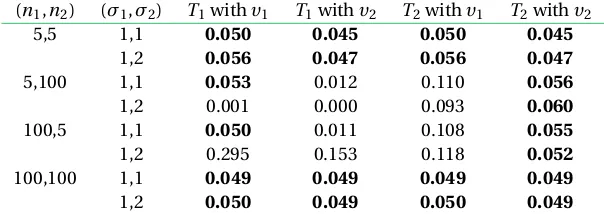
To demonstrate the impact of the degrees of freedom, for insight only, the independent samples t-testT1but with υ2degrees of freedom is considered. Likewise, for insight only, Welch’s test using statisticT2but withυ1degrees of freedom is considered. These are compared against the standard approaches for the independent samples t-test and Welch’s test. Table 2 summarises the Type I error rates observed (α=.05, two-sided) for each combination. Bradley’s (1978) liberal robustness criteria states that the Type I error rate when the nominalαis .05 should be in the range {0.025, 0.075}.
Table2shows that Welch’s test (test statistic and degrees of freedom ) is Type I error robust across all scenarios simu-lated. For unequal sample sizes and unequal variances,T1 used in conjunction withυ1orυ2, andT2used in conjunc-tion withυ1, do not meet liberal robustness criteria. Welch’s
degrees of freedom therefore represent an important prop-erty for controlling Type I error rates. However, clearly the calculation of the test statistic, which takes into account the two separate sample variances, is also important.
Impact of the standard error on the properties of Welch’s test.
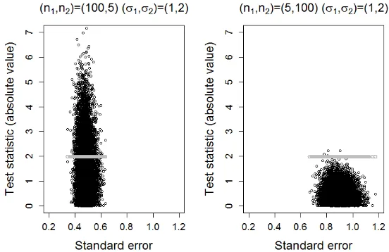
In this section, the impact of the standard error of the test statistics for the independent samples t-test and Welch’s test is considered. The corrective properties of Welch’s test are, in part, due to the impact of the sample variances on the degrees of freedom, which in turn affects the critical value used in the test. However, Type I error robustness could also be due to the impact of the estimated standard error on the magnitude of the test statistic. Figure4and Figure5demonstrate how the standard error,SE1andSE2, relate to the critical value and to the absolute values of the test statistic for the independent samples t-test,T1, and Welch’s test,T2, respectively.
Both panels of Figure4suggest that, when performing the independent samples t-test, the estimated standard er-ror,SE1, has no apparent relationship with the value of the test statistic,T1. When the smaller sample size is associ-ated with the larger population variance (left panel, Figure 4), the absolute value of the test statistic has a larger mean and a larger variability. When the larger sample size is asso-ciated with the larger population variance (right panel, Fig-ure4), the absolute value of the test statistic has a smaller mean and a smaller variability. This has the result that more false positives are observed when the smaller sample size is associated with the larger variance.
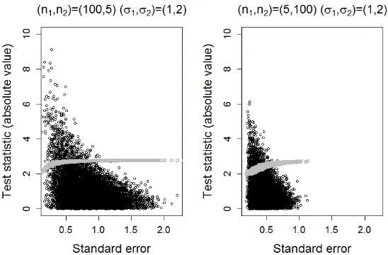
Both panels of Figure5demonstrate the impact of the degrees of freedom on the critical value. In the simulated scenario; the theoretical minimum degrees of freedom is mi n(n1,n2)=4, accordingly the upper bound of the criti-cal value is 2.776; the theoreticriti-cal maximum degrees of free-dom isυ1=98, accordingly the lower bound of the critical value is 1.984.
It can be seen from both panels of Figure 5 that as Welch’s estimate of standard error,SE2, increases, the ab-solute value ofT2decreases. As the estimated standard er-ror becomes large, the impact is far greater on the absolute value ofT2relative to the critical value. This combination results in fewer false positives being observed as the
esti-TheQuantitativeMethods forPsychology 33
Figure 1 Distribution ofυ2for each scenario. The references lines represent the theoretical maximum and minimum values thatυ2can take. The upper reference line is equivalent toυ1.
mated standard error increases.
Discussion
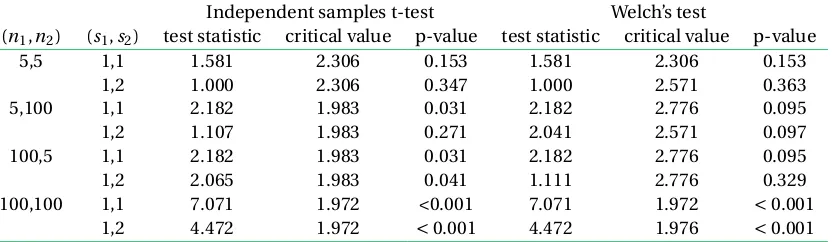
For additional clarity of the above findings, Table3 sum-marises theoretical values for each of the combinations in the simulation design. For illustration purposes differences in means are fixed at 1.000,s1ands2are fixed asσ1andσ2 respectively.
From Table3, it can be seen that when sample sizes are equal or variances are equal, the test statistics for the in-dependent samples t-test and Welch’s test are equivalent. Therefore, the difference in p-values are a direct result of the degrees of freedom used to calculate the critical value.
When variances are not equal, Welch’s estimated stan-dard error impacts the critical value, but this effect is smaller than the effect on the value on the test statistic. When the smaller sample size is associated with the larger variance, the effect on the value of the test statistic is
exac-erbated.
Conclusion
The literature favours Welch’s test for a comparison of two means. This paper adds further support to the findings in the literature with respect to the Type I error robustness of Welch’s test. The degrees of freedom of Welch’s test are a random variable based on the sample size and variance of each sample. The degrees of freedom used in Welch’s test are always less than or equal to the degrees of freedom used in the independent samples t-test. The degrees of freedom used in the independent samples t-test and Welch’s test are equivalent whens21/s22={(n1−1)n1}/{(n2−1)n2}. The min-imum value of Welch’s degrees of freedom ismi n{n1,n2}− 1, this minimum is determined by the sample with the larger variance. Therefore Welch’s approximate degrees of freedom are more conservative than the degrees of freedom used in the independent samples t-test, particularly when
TheQuantitativeMethods forPsychology 34
Figure 2 Value ofυ2with varyings22, and fixed values12=1. Values to the left ofs22=1 have the larger variance associated with Sample 1. Values to the right ofs22=1 have the larger variance associated with Sample 2.
Table 2 Type I error rates for each combination of test statistic with degrees of freedom. Type I error robust combinations are highlighted in bold.
(n1,n2) (σ1,σ2) T1withυ1 T1withυ2 T2withυ1 T2withυ2
5,5 1,1 0.050 0.045 0.050 0.045
1,2 0.056 0.047 0.056 0.047
5,100 1,1 0.053 0.012 0.110 0.056
1,2 0.001 0.000 0.093 0.060
100,5 1,1 0.050 0.011 0.108 0.055
1,2 0.295 0.153 0.118 0.052
100,100 1,1 0.049 0.049 0.049 0.049
1,2 0.050 0.049 0.050 0.049
the smaller sample size is associated with the larger vari-ance. When performing Welch’s test, the estimated stan-dard error impacts the magnitude of the test statistic. Un-der the null hypothesis, it is the estimated standard error when performing Welch’s test, which is the most influential factor on the result of the test. For Welch’s test, the prob-ability of making a Type I error decreases as the standard error increases. This paper gives insight in to why Welch’s test is Type I error robust for normally distributed data, in scenarios when the independent samples t-test is not. Ad-ditionally, it is shown that in situations when the indepen-dent samples t-test is Type I error robust, Welch’s test is also. In a practical environment for the comparisons of two means from assumed normal populations, a general rule to preserve Type I error robustness is, if in doubt use Welch’s test.
References
Alfassi, Z. B., Boger, Z., & Ronen, Y. (2005).Statistical treat-ment of analytical data. CRC Press.
Aspin, A. A. (1948). An examination and further develop-ment of a formula arising in the problem of compar-ing two mean values.Biometrika. 2, 88–96. doi:10 . 2307/2332631
Aspin, A. A. (1949). Tables for use in comparisons whose ac-curacy involves two variances, separately estimated. Biometrika. 36, 290–296. doi:10.2307/2332668 Behrens, W. U. (1929). Ein beitrag zur fehlerberechnung
bei wenigen beobachtungen. Landwirtschaftliche Jahrbucher. 68, 807–837.
Best, D. J. & Rayner, J. C. W. (1987). Welch’s approximate so-lution for the behrens-fisher problem.Technometrics. 29(2), 205–210. doi:10.2307/1269775
TheQuantitativeMethods forPsychology 35
[image:6.612.56.358.393.500.2]Figure 3 P-values for the independent samples t-test,T1, and Welch’s test,T2. The left panel shows the smaller sample size associated with the larger variance. The right panel shows the larger sample size associated with the larger variance.
Table 3 Components of the tests for each scenario in the simulation design.
Independent samples t-test Welch’s test
(n1,n2) (s1,s2) test statistic critical value p-value test statistic critical value p-value
5,5 1,1 1.581 2.306 0.153 1.581 2.306 0.153
1,2 1.000 2.306 0.347 1.000 2.571 0.363
5,100 1,1 2.182 1.983 0.031 2.182 2.776 0.095
1,2 1.107 1.983 0.271 2.041 2.571 0.097
100,5 1,1 2.182 1.983 0.031 2.182 2.776 0.095
1,2 2.065 1.983 0.041 1.111 2.776 0.329
100,100 1,1 7.071 1.972 <0.001 7.071 1.972 <0.001
1,2 4.472 1.972 <0.001 4.472 1.976 <0.001
Bland, M. (2013). Do baseline p-values follow a uniform distribution in randomised trials? PloS one, 8(10), e76010. doi:10.1371/journal.pone.0076010
Bradley, J. V. (1978). Robustness?British Journal of Math-ematical and Statistical Psychology. 31(2), 144–152. doi:10.1111/j.2044-8317.1978.tb00581.x
Coombs, W. T., Algina, J., & Oltman, D. (1996). Univari-ate and multivariUnivari-ate omnibus hypothesis tests se-lected to control type i error rates when popula-tion variances are not necessarily equal. Review of Educational Research. 66(2), 137–79. doi:10 . 3102 / 00346543066002137
Fagerland, M. W. & Sandvik, L. (2009). Performance of five two-sample location tests for skewed distributions with unequal variances.Contemporary Clinical Trials. 30(5), 490–496. doi:10.1016/j.cct.2009.06.007
Fairfield-Smith, H. (1936). The problem of comparing the results of two experiments with unequal errors. Jour-nal of the Council for Scientific and Industrial Re-search,9, 211–212.
Fay, M. P. & Proschan, M. A. (2010). Wilcoxon-mann-whitney or t-test?On assumptions for hypothesis tests and multiple interpretations of decision rules. Statis-tics Surveys. 4(1), 1. doi:10.1214/09-SS051
Fisher, R. A. (1935). The fiducial argument in statistical in-ference.Annals of Eugenics.391–398. doi:10 . 1111 / j . 1469-1809.1935.tb02120.x
Fisher, R. A. (1941). The asymptotic approach to behrens’ integral, with further tables for the d test of signifi-cance.Annals of Eugenics. 11, 141–172. doi:10 . 1111 / j.1469-1809.1941.tb02281.x
Frank, H. & Althoen, S. C. (1994).Statistics: concepts and ap-plications. Cambridge University Press.
TheQuantitativeMethods forPsychology 36
[image:7.612.63.479.379.500.2]Figure 4 Simulated values of the standard error,SE1, against the absolute value of the test statistic,T1, for the indepen-dent samples t-test. The critical value, a constant at 1.984, has been superimposed. The left panel shows the smaller sample size associated with the larger variance. The right panel shows the larger sample size associated with the larger variance.
Grimes, B. A. & Federer, W. T. (1982).Comparison of means from populations with unequal variances. Biometrics Unit Technical Reports: Number BU-762-M.
Lee, A. F. S. & Gurland, J. (1975). Size and power of tests for equality of means of two normal populations with unequal variances.Journal of the American Statistical Association. 70(352), 933–941. doi:10.1080/01621459. 1975.10480326
Miles, J. & Banyard, P. (2007). Understanding and using statistics in psychology: a practical introduction. Sage. Moser, B. K., Stevens, G. R., & Watts, C. L. (1989). The two-sample t test versus satterthwaite’s approximate f test. Communications in Statistics-Theory and Methods. 18(11), 3963–3975. doi:10.1080/03610928908830135 Ott, R. L. & Longnecker, M. (2001).An introduction to
sta-tistical methods and data analysis. Pacific Grove, CA: Duxbury.
Phillips, L. T. & Lowery, B. S. (2015). The hard-knock life? whites claim hardships in response to racial inequity. Journal of Experimental Social Psychology,61, 12–18. doi:10.1016/j.jesp.2015.06.008
R Development Core Team. (2013).R: a language and en-vironment for statistical computing. ISBN 3-900051-07-0. R Foundation for Statistical Computing. Vienna, Austria. Retrieved fromhttp://www.R-project.org Rasch, D., Kubinger, K., & Yanagida, T. (2011).Statistics in
psychology using r and spss. John Wiley and Sons.
Ruxton, G. (2006). The unequal variance t-test is an un-derused alternative to student’s t-test and the mann-whitney u test. Behavioral Ecology. 17(4), 688–690. doi:10.1093/beheco/ark016
Satterthwaite, F. E. (1946). An approximate distribution of estimates of variance components. Biometrics Bul-letin. 2, 110–114. doi:10.2307/3002019
Sawilowsky, S. S. & Blair, R. C. (1992). A more realistic look at the robustness and type ii error properties of the t-test to departures from population normality. Ameri-can Psychological Association. 111(2), 352–360. doi:10. 1037/0033-2909.111.2.352
Scheffe, H. (1970). Practical solutions of the behrens-fisher problem.Journal of the American Statistical Associ-ation. 65, 1501–1508. doi:10 . 1080 / 01621459 . 1970 . 10481179
Wang, Y. Y. (1971). Probabilities or the type l errors of the welch tests for the behrens-fisher problem. Journal of the American Statistical Association. 66, 605–608. doi:10.1080/01621459.1971.10482315
Welch, B. L. (1938). The significance or the difference between two means when the population variances are unequal.Biometrika. 29, 350–362. doi:10 . 2307 / 2332010
Welch, B. L. (1947). The generalization of ’student’s’ prob-lem when several different population variances are involved.Biometrika. 34, 28–35. doi:10.2307/2332510
TheQuantitativeMethods forPsychology 37
Figure 5 Properties of Welch’s test. The critical values have been superimposed. The left panel shows the smaller sample size associated with the larger variance. The right panel shows the larger sample size associated with the larger variance.
Welch, B. L. (1951). On the comparison of several mean val-ues: an alternative approach.Biometrika. 38, 330–336. doi:10.2307/2332579
Wilcox, R. R. (1992). Why can methods for comparing means have relatively low power, and what can you do to correct the problem?Current Directions in Psycho-logical Science. 1(3), 101–105.
Zimmerman, D. W. & Zumbo, B. D. (1993). Rank transfor-mations and the power of the student t-test and welch
t-test for non-normal populations. Canadian Jour-nal of Experimental Psychology. 47(3), 523–39. doi:10. 1037/h0078850
Zimmerman, D. W. & Zumbo, B. D. (2009). Hazards in choosing between pooled and separate-variances t-tests.Psicológica: Revista de metodología y psicología experimental,30(2), 371–390.
Citation
Derrick, B., Toher, D., & White, P. (2016) Why Welch’s test is Type I error robust. .The Quantitative Methods for Psychology, 12(1), 30-38.
Copyright© 2016 Derrick, Toher, & White. This is an open-access article distributed under the terms of the Creative Commons Attribution License (CC BY). The use, distribution or reproduction in other forums is permitted, provided the original author(s) or licensor are credited and that the original publication in this journal is cited, in accordance with accepted academic practice. No use, distribution or reproduction is permitted which does not comply with these terms.
Received: 28/08/2015∼Accepted: 12/10/2015
TheQuantitativeMethods forPsychology 38