Edge Detection Based on Improved Non Maximum Suppression Method



Abstract: Semantic Segmentation and edge detection are important research fields for scene understanding in computer vision. A hierarchical framework called Contextual Hierarchical Model (CHM) was proposed for semantic image segmentation and edge detection. It learned contextual information using a Logistic Disjunctive Normal Networks (LDNN) classifier. The class average accuracy of CHM was improved by defining a global constraint using Conditional Random Field (CRF), Hierarchical CRF (HCRF), Higher order HCRF (HHCRF). The LDNN was improved by using proximal gradient method which minimizes the quadratic error and it had high convergence rate than gradient descent method. The weight and bias terms of LDNN was optimized by using Grey Wolf Optimization algorithm (GWO) which improves the classification accuracy and it also reduces time complexity of LDNN. During the edge detection using CHM, a multi-scale strategy was adopted to compute edge maps. A Non-Maximum Suppression (NMS) was used to obtain the thinned edges in images. However, it is a post-processing step which consumes additional time in edge detection process. So, in this paper, the edge detection is interpreted as a classification problem where the thinned edges in images are obtained without any post-processing step. It reduces the time consumption. Two key ingredients such as loss and joint processing are included in NMS to improve the detection of thinned edges. The loss is used to penalize the double edge detection and the joint processing is used to reduce the loss of edge detection by including a pair features as additional feature for edge detection. The pair features, Haar, Histogram of Gradient (HOG) and SIFT features are given as input to LDNN to detect the edges that improve the efficiency of CHM based edge detection.

Index Terms: Semantic Image Segmentation, Edge Detection, Non-Maximum Suppression, Post-Processing.

I. INTRODUCTION

Image segmentation [1] is the process of partitioning an image into number of regions or set of pixels. The outcome of the image segmentation process is a set of contours or regions that collectively covers the whole image. Based on some characteristics or computed property, such as intensity, color or texture the pixels are grouped in a region. Neighboring regions are significantly dissimilar with respect to same characteristics. Semantic image segmentation process [2] not only realizes what objects are in an image but it also used to locate objects in an image. It divides an image into a finite number of non-overlapping and meaningful regions. Edge detection is one of the important processes in semantic image segmentation.

Revised Manuscript Received on July 10, 2019.

Sreedhar.T, Ph.D Research Scholar, Department of Computer Science, Erode Arts & Science College (Autonomous), Erode, India.

Sathappan.S, Research Supervisor and Associate Professor, Department of Computer Science, Erode Arts & Science College (Autonomous), Erode, India.

.

Edge detection [3] is the process of finding and locating sharp discontinuities in an image. Often, the edges of object planes in an image provide the oriented localized changes in the intensity of that image. Edge detection techniques convert an original image into edge image assisting from the changes of grey tones in the images. The outcome of this transformation returns an edge image without changing any physical qualities of the original image. Based on the detected edges, the objects in images are segmented.

A contextual framework called contextual hierarchical model (CHM) [4] was proposed for semantic image segmentation. The contextual information of an input image was learned in a hierarchical framework. It consists of multiple hierarchy levels where a Logistic Disjunctive Normal Networks (LDNN) was trained at each level of hierarchy based on down sampling input images and outputs of previous levels. Then multi-resolution contextual information from each level was combined into a classifier to segment the input image at original resolution. Even though CHM is able to model contextual information within a scene, it can be prone to errors due to the absence of global constraints. Due to the absence of global constraint, the CHM has poor performance in terms of class average accuracy.

So, the global constraint for CHM was defined through different models such as Conditional Random Field (CRF), Hierarchical CRF (HCRF) and HCRF with higher-order features (HHCRF) [5] where energy functions were defined on a discrete random field. The CRF, HCRF, and HHCRF were processed in the bottom-up step of CHM and its result was utilized to train LDNN. It segmented the images semantically within the top down steps of CHM. A gradient descent was utilized in LDNN to minimize the quadratic error. It has slow convergence rate which can affect the efficiency of LDNN.

So, CHM- HHCRF- Improved LDNN (CHM- HHCRF- ILDNN) [6] was proposed where a proximal gradient method is used to minimize the quadratic error which has a faster convergence rate. Moreover, CHM-HHCRF- Improved Optimized LDNN (CHM-HHCRF-IOLDNN) was proposed to optimize the weight and bias term of LDNN using Grey Wolf Optimization algorithm (GWO) [7] which improves the classification accuracy. The thinned edges in the images were detected by CHM-HHCRF-IOLDNN using standard Non-Maximum Suppression (NMS). NMS is processed as a post-processing and it takes a longer time to detect the edges.

So, in this paper, a CHM is designed without any post processing for edge detection. The edge detection based on NMS is improved by including two key 0. Such as, loss and joint processing to build an NMS. A loss that penalizes double edge detection and

the joint processing of edge detection reduces the loss of edge detection. In the joint

Edge detection based on Improved

Non-Maximum Suppression Method

processing, a pair of features in images are included and it is given as additional feature along with the features such as Haar, Histogram of Gradients (HOG) and SIFT to CHM-HHCRF-IOLDNN for edge detection. Hence, NMS without post-processing reduces the time consumption and two key ingredients improve the accuracy of CHM-HHCRF-IOLDNN based edge detection.

II. LITERATURESURVEY

Based on Neutroscopic Set (NS) structure, an edge detection method [8] was proposed. This method was started with split an image into T, I and F subsets. Then, these subsets were undergoing the edge detection process. The edges in the images were related to the indetermination situations. So, NS was utilized to analysis the edges of images. T and F subsets were identified by using entropy those subsets were considered as significant elements in edge detection with NS. However, the entropy used in this method has an impact on the edge detection results.

Using a modified Moore-Neighbor algorithm, an edge detection method [9] was proposed. It is also called as 8-Neighborhood. For boundary detection and feature extraction, the modified Moore-Neighbor algorithm was used as boundary tracing. In this algorithm a set of 8 pixels shared its vertex or edge with a pixel. In order to detect the edges of objects in the images, a range of filter was integrated with the modified Moore-Neighbor algorithm. However, this method still has poor Baddeley’s Delta Metric at some point of variance.

For edge detection, a novel Convolutional Neural Network (CNN) based pipeline [10] was presented. It integrated multi-level information in a feature map-based manner. The multi-level information was extracted from different intermediate layers creating Hybrid Convolutional Features (HCF). These features were fed into the edge detector which detected edges without post-processing. Although this method achieves 22fps speed, it is not a real edge detector. Based on feature re-extraction (FRE) of a deep convolutional neural network, an edge detector [11] was proposed for edge detection of objects in images. This edge detector was comprised of backbone, side-output and feature fusion modules. The backbone module extracted preliminary features from an image. The side-output module applied residual learning to make network architecture more robust by mapping features from various stages of the backbone network with edge-pixel space. The edge map was generated in the feature fusion module. However, the computational complexity of this edge detector is high.

Based on Computational Ghost Imaging (CGI), an optical edge detection method [12] was proposed for edge detection. It recognized the features of an object in the image. The CGI with standard illumination was generated by using an interference system. Furthermore, structured intensity patterns were designed to directly map the detected data in CGI with the edge of an object. The optical edge detection method extracted the boundaries for grayscale and binary objects in any direction at one time. However, this method extracted boundaries sharp and clearly visible only up to deviation 5mm.

For semantic image segmentation, a hybrid Bayesian Network (BN) model and Hierarchical Conditional Random Field model (HCRF) [13] were proposed. HRCF

generated initial semantic sub-scene prediction by capturing non-casual relationship whereas BN modeled contextual interactions for each semantic sub-scene. From the training data, the conditional probabilities of contextual interactions were. Then, the structure of contextual dependencies was encoded in the initial predictions from learned BN structure to create final refined predictions. However, this method has low accuracy.

For semantic image segmentation of remote sensing harbor images, an edge aware deep convolutional neural network [14] was proposed. The segmentation and edge detection networks were trained simultaneously by designing a multitask model. The edge network was learned from the extracted hierarchical semantic features. The entire model was further refined by adding the outputs of edge pipeline with an edge-aware regularization. However, a user-defined parameter was used to adjust the weight of regularization term that greatly influences the segmentation results.

III. METHODOLOGY

In this section, edge detection using standard Non-Maximum Suppression (NMS) and NMS without post-processing are described in detail. The post-processing consumes more time and hence the edge detection process takes a longer time to detect the thinned edges. So, a CHM is designed with NMS without post processing and two key ingredients such as loss and joint processing are introduced in NMS to improve the efficiency of edge detection.

A. Standard NMS method for edge detection

Non-Maximum Suppression (NMS) works by finding the pixel with the maximum value in an edge. NMS is carried out to preserve all local maxima in the gradient image and deleting everything else which results in thin edges. NMS consists of:

 Consider a point , where and are pixel integers and be the intensity of pixel .  Calculate the gradient of image intensity and its

magnitude in .

 Estimate the magnitude of the gradient along the direction of the gradient in some neighborhood

around .

 If is not a local maximum of the magnitude of the gradient along the direction of the gradient then it is not an edge point.

B. NMS without Post-processing

The standard NMS gets input as window, window associated edge class labels and window network response score. Then it removes those windows which are not locally the highest-scored, to yield a final set of edge detections. It is processed as a post-processing step in CHM to obtain the thinned edges. It consumes additional time to detect the edges. In order to reduce the time consumption, learn the NMS into the classifier. For every possible detection in an image, it computes the probabilities of edge classes. It gives rise to score detectors which develop a search space of detection. Then class probabilities were computed for each edge detection. Accordingly, two strongly overlapping edges in the image will both result

coverage capacity of detection windows, each contents in the image triggers various edge detections of varying confidence.

NMS creates high confidence edge detections in which it is considered that the highly overlapping edge detections belong to the same image pixel and combine them into one edge detection. The IOLDNN classifier differentiates the image content that contains an edge and the image content that does not contain an edge. In the training data of IOLDNN for edge detection, the positive and negative samples are defined by some measure of overlap between edges and windows. Since similar window will generate similar confidence, a small perturbation of edge locationsis considered positive samples. However, the trained IOLDNN classifier does not provides one high scoring edge detection. It encourages multiple high scoring edge detections.

In order to generate exactly one edge detection, two key ingredients are considered. One of the ingredients is a loss that penalizes double detections to teach the detector precisely. Another ingredient is the joint processing of neighboring detections so the detector has the necessary information to define whether an edge is detected multiple times.

IOLDNN based edge detector is supposed to return exactly one high scoring edge detection. The loss for such a detector must restrain multiple edge detections of the same image pixel, irrespective of how close these detections are. A matching strategy is used to ensure the results of NMS based multiple edge detections. The IOLDNN detector is judged by the evaluation criterion of a benchmark, which in turn describes a matching strategy to decide which edge detections are correct or wrong. This strategy is used during the training stage of the edge detection. Based on the edge detection confidence, benchmarks sort detection in descending order. Then, in the sorted order match the edge detection to image pixels. In this matching strategy, already matched image pixels cannot be matched again and the remaining edge detections are counted as false positives that decrease the precision of IOLDNN based edge detection. The results of this matching strategy are used as labels for the IOLDNN to detect the thinned edges.

All detections that are used for training of a classifier have a label as they are given as input to the IOLDNN network. In such situation, this network has access to edge detections and image pixel annotations. The matching strategy creates labels that depend on the prediction of the network. Consider is a detection, indicate whether is successfully matched or not to an image pixel and denotes the scoring function that jointly scores all

detections on an image , where

denotes the number of edge detections. This is trained with the weighted logistic loss

In the above equation, matching strategy is used to couple the loss per edge detection with the other edge detections. The matching produces and is used to counter act the extreme class imbalance of the edge detection task. The IOLDNN detects the thinned edges by minimizing the weighted logistic loss.

Each IOLDNN consists of edge detections on an image each edge detections are represented by a dimensional feature vector. A detection context layer is used for every detection , generates all pairs of detections for which sufficiently overlaps with . The representation of a pair of detections consists of the concatenation of both detection representations and -dimensional detection pair features which yields an dimensional feature. The pair features consist of several properties of a detection pair are the intersection over union, the normalized distance in and -direction and the normalized distance, scale difference of width and height and difference of aspect ratio are used as pair features in pairwise context. The features of all pairs of detections are arranged to process each pair of edge detections independently. If edge detection has neighboring edge detection that yields a size , where

since the pair is also included. The max pooling is used to reduce the variable sized neighborhood into a fixed size representation. The pair features of pairwise context are also given as additional input to the IOLDNN which improves the efficiency of the edge detection process.

IV. RESULTANDDISCUSSION

In this section, experimental studies are carried out in Berkeley Segmentation Dataset (BSDS) to evaluate the

performance of CHM-HHCRF-NMS-IOLDNN and

CHM-HHCRF-INMS-IOLDNN based edge detection in terms of average precision, for the whole dataset fixed threshold value F-measure is quantified (ODS) and pixel accuracy. The BSDS consists of 500 images in which 200 images are used for training, 100 images are used for validation and the remaining images are used for testing.

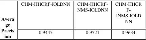
The comparison of average precision between Contextual Hierarchical Model- Higher order Hierarchical Conditional Random Field-Improved Optimized Logistic Disjunctive

Normal Networks (CHM-HHCRF-IOLDNN), CHM-

HHCRF- Non-Maximum Suppression-IOLDNN (CHM - HHCRF - NMS - IOLDNN) and CHM-HHCRF- Improved NMS-IOLDNN (CHM-HHCRF-INMS-IOLDNN) on BSDS 500 dataset is given in Table I.

Table I Comparison of Average Precision

Avera ge Precis

ion

CHM-HHCRF-IOLDNN CHM-HHCRF- NMS-IOLDNN

CHM-HHCR F- INMS-IOLD

NN

0.9445 0.9521 0.9634

As shown in Table I and Fig. 1, the proposed CHM without post-processing (CHM-HHCRF-INMS-IOLDNN) model achieves the state-of-the-art performance. In CHM-HHCRF-IOLDNN, the thinned edges are not detected. In the CHM-HHCRF-NMS-IOLDNN model, NMS is done as the post processing process to detect the thinned edges. In order to have true end-to-end

The detectors with post-processing has impact on the performance in terms of average precision which is clearly shown in Table I and Fig. 1. The proposed CHM-HHCRF-INMS-IOLDNN detects the edges of the objects without any post-processing with average precision of 0.9634 where the NMS is included into the classification process. The CHM-HHCRF-NMS-IOLDNN detects the edges with post-processing with average precision of 0.9521. The CHM-HHCRF-IOLDNN detects the edges with average precision of 0.9445. The average precision of CHM-HHCRF-INMS-IOLDNN is 2% greater than average precision of CHM-HHCRF-IOLDNN and 1.2% greater than average precision of CHM-HHCRF-NMS-IOLDNN. From this analysis, it is known that the proposed CHM-HHCRF-INMS-IOLDNN has high average precision

than the CHM-HHCRF-IOLDNN and

CHM-HHCRF-NMS-IOLDNN.

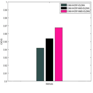
Fig. 1 Comparison of Average Precision

The comparison of ODS between

CHM-HHCRF-IOLDNN, CHM-HHCRF-NMS-IOLDNN

and CHM-HHCRF-INMS-IOLDNN on BSDS 500 dataset is given in Table II.

Table II Comparison of ODS

Number of levels in

CHM

CHM-HHCRF -IOLDNN

CHM-HHCRF- NMS-IOLDNN

CHM-HHCRF- INMS-IOLDNN

0 88 88.5 90

1 92

92.4

94

2 95 95.81 96.12

3 97 97.7 98.56

4 98.6 98.82 98.94

5 98.79 98.84 99

From Table II and Figure. 2, it is found that the proposed CHM-HHCRF-INMS-IOLDNN method has better F-value with fixed threshold value (ODS) than CHM- HHCRF- IOLDNN and CHM-HHCRF- NMS- IOLDNN. The ODS value of CHM-HHCRF-INMS-IOLDNN is improved by interpreting the thinned edge detection based on

NMS as a classification problem where the thinned edges in the images are detected more effectively. The loss ingredient of INMS encourages exactly only one edge detection per object for overlapping edges in the images which greatly enhance the edge detection in terms of ODS. The ODS of CHM-HHCRF-INMS-IOLDNN is 2.73% more than ODS of CHM-HHCRF-IOLDNN and 1.46% more than ODS of CHM-HHCRF-NMS-IOLDNN. From this analysis, it is known that the proposed CHM-HHCRF- INMS- IOLDNN has high ODS than the CHM-HHCRF-IOLDNN and CHM-HHCRF-NMS- IOLDNN.

Fig. 2 Comparison of ODS

Table III Comparison of Pixel Accuracy

ODS

CHM-HHCRF -IOLDNN

CHM-HHCRF- NMS-IOLDNN

CHM-HHCRF - INMS-IOLDNN

0.9418 0.9536 0.9675

Table III shows the comparison of pixel accuracy between CHM-HHCRF-IOLDNN, CHM-HHCRF-NMS- IOLDNN and CHM-HHCRF-INMS-IOLDNN on BSDS 500 dataset under different number of levels in CHM.

Fig.3 shows the comparison of pixel accuracy between CHM-HHCRF-IOLDNN, CHM-HHCRF-NMS- IOLDNN and CHM-HHCRF-INMS- IOLDNN based edge detection. The different number of levels is taken in X-axis and the pixel accuracy is taken in Y-axis. By including pair features of each detection pair in CHM-HHCRF- INMS-IOLDNN, the true positive and true negative rate for edge detection is improved. In addition to this, NMS with loss and joint processing for penalizing the double edge detection and to check whether the edges are detected multiple times enhance the pixel accuracy of edge detection process. When the number of levels in CHM is 1, the pixel accuracy of CHM- HHCRF- INMS-IOLDNN is 2.17% more than pixel accuracy of CHM-HHCRF-IOLDNN and 1.73% more than pixel accuracy of CHM-HHCRF-NMS-IOLDNN. From this analysis, it is concluded that

pixel accuracy than the CHM-HHCRF-IOLDNN and CHM-HHCRF-NMS- IOLDNN.

Fig. 3 Comparison of Pixel Accuracy

The performance of CHM-HHCRF-IOLDNN, CHM-HHCRF-NMS-IOLDNN and CHM-HHCRF-INMS- IOLDNN for 4 sample images of BSDS dataset is shown in Fig. 4. Fig. 4a shows the input images which have 256 256 resolution. Fig. 4b shows the ground truth image of the input image. Fig. 4c shows the output of CHM-HHCRF-IOLDNN method. Fig. 4d shows the output of CHM-HHCRF- NMS-IOLDNN method and Fig. 4e shows the output of CHM-HHCRF-INMS-IOLDNN method.

V. CONCLUSION

In this paper, the NMS based edge detection in CHM is improved by including loss and joint processing in the edge detection process. Initially, the edge detection is

deduced as a classification problem. The NSM based edge detection method was providing multiple detections for a single object. In order to provide a single edge detection of an object with a high score, a weighted logistic loss is included in NMS. In the joint processing, concatenates the detection representation and pair features which yield new dimensional features. It is given as additional input to LDNN along with Haar, Histogram of Gradient (HOG) and SIFT features which enhance the performance of NMS based edge detection in CHM. The experiments are conducted in Berkley Segmentation Dataset that shows that the proposed

CHM-HHCRF-INMS-IOLDNN based edge detection

o

o

(a) (b) (c) (d) (e)

Fig. 4 Test Samples of Berkeley segmentation dataset (BSDS 500). (a) Input image, (b) Ground Truth Image, (c) CHM-HHCRF-IOLDNN, (d) CHM-HHCRF-NMS-IOLDNN, (e) CHM-HHCRF-INMS-IOLDNN.

REFERENCES

1. Khan, W. (2013). Image Segmentation Techniques: A Survey. Journal of Image and Graphics, 1(4), 166-170.

2. Liu, X., Deng, Z., & Yang, Y. (2018). Recent progress in semantic image segmentation. Artificial Intelligence Review, 1-18.

3. Muthukrishnan, R., & Radha, M. (2011). Edge detection techniques for image segmentation. International Journal of Computer Science & Information Technology, 3(6), 259.

4. Seyedhosseini, M., & Tasdizen, T. (2016). Semantic image segmentation with contextual hierarchical models. IEEE transactions on pattern analysis and machine intelligence, 38(5), 951.

5. Sreedhar, T., & Sathappan, S. (2018). Different Conditional Random Field based Contextual Hierarchical model for Semantic Image Segmentation.

6. Sreedhar, T., & Sathappan, S. (2018). An Improved Optimized Logistic Disjunctive Normal Network Classifier for Efficient Semantic Image Segmentation.

7. Singh, N., & Singh, S. B. (2017). A Modified Mean Gray Wolf Optimization Approach for Benchmark and Biomedical Problems.

Evolutionary Bioinformatics, 13, 1176934317729413.

8. Eser, S. E. R. T., & Derya, A. V. C. I. (2019). A new edge detection approach via neutrosophy based on maximum norm entropy. Expert Systems with Applications, 115, 499-511.

9. Biswas, S., & Hazra, R. (2018). Robust edge detection based on Modified Moore-Neighbor. Optik, 168, 931-943.

10. Hu, X., Liu, Y., Wang, K., & Ren, B. (2018). Learning Hybrid Convolutional Features for Edge Detection. Neurocomputing. 11. Wen, C., Liu, P., Ma, W., Jian, Z., Lv, C., Hong, J., & Shi, X. (2018).

Edge detection with feature re-extraction deep convolutional neural network. Journal of Visual Communication and Image Representation, 57, 84-90.

12. Yuan, S., Xiang, D., Liu, X., Zhou, X., & Bing, P. (2018). Edge detection based on computational ghost imaging with structured illuminations. Optics Communications, 410, 350-355.

13. Wang, L. L., & Yung, N. H. (2015). Hybrid graphical model for semantic image segmentation. Journal of Visual Communication and Image Representation, 28, 83-96.

14. Cheng, D., Meng, G., Xiang, S., & Pan, C. (2017). FusionNet: Edge Aware Deep Convolutional Networks for Semantic Segmentation of Remote Sensing Harbor Images. IEEE Journal of Selected Topics in Applied Earth Observations and Remote Sensing, 10(12), 5769-5783.

AUTHORSPROFILE

T.Sreedhar received the MCA degree from Anna University, India in the year 2011 and M.Phil degree in Computer Science from Bharathiar University, India in the year 2015 respectively. Currently, he is a Full-Time Ph.D., Research Scholar of Computer Science, Erode Arts and Science College, Erode, affiliated to Bharathiar University. He also worked as an Assistant Professor with the total experience of 5 years. He has published one papers in International Conferences, one papers in UGC Journal and one paper in

Scopus indexed Journal. His area of interest is image processing. Email: [email protected]

Dr.S.Sathappan received the M.Sc., degree in Applied Mathematics from Bharathidasan University, India in the year 1984, the MPhil and PhD degrees in Computer Science from Bharathiar University, India in the year 1996 and 2012 respectively. Currently, he is an Associate Professor of Computer Science, Erode Arts and Science College, Erode, Affiliated to Bharathiar University, Coimbatore. He served as a Syndicate Member of Bharathiar University from June 2015 to June 2018. He also Served as a Senate Member of Bharathiar University

2005-2008 and 2015-2018. He has been a supervisor for several students of MCA/MPhil., programs over the past several years. Also, he has guided 6 Ph.D Scholars and guiding 6 Ph.D Scholars . He has a total experience of over 33 years. He has published 32 papers in Conferences and 41 papers in Journal. His areas of interest include computer simulation and image processing.