Shortest Path Problems Using Fuzzy Weighted Arc Length

(1)

Abstract: We have presented a novel method for solving the fuzzy shortest path problem (FSPP) considering Type-I and Type-II weighted trapezoidal fuzzy number (WTpFN) and weighted triangular fuzzy number (WTrFN) and also can predict the crisp shortest path (CSP) length. Additionally, the method is compared with some existing methods. Finally, we have given some numerical experiments to show the effectiveness of the proposed model. Numerical and graphical results show that the new technique is superior to the current methods.

Index Terms: Weighted trapezoidal fuzzy numbers, fuzzy linear programming, ranking method, fuzzy shortest path problem.

I.INTRODUCTION

There are many situations in real life where we need to find the shortest path (SP) from origin to destination. Traditionally, fundamental graph theory can solve SPP when the parameters (such as time, cost, distance and so on) are a crisp number. For example, Dijkstra's algorithm [1] where the weighted graph is used to find the SP. Bellman-Ford algorithm [2] used the single-source problem to find the SP when edge weight is negative. Floyd–Warshall algorithm [2] solved all SPs in pair.but there are many situations in real life where we have to face with uncertain parameters such as natural calamities (flood, earthquake, heavy rainfall, low visibility during winter) or social disasters such as strike, roadblock or bad human health which may act as hurdle between the origin to destination.To remove these uncertainties from the above mentioned cases, we utilise Zadeh's fuzzy [3] principle. When the SP problem is solved under the fuzzy environment, then such type of problem is known as FSPP. During the last few decades, the topic of FSPP has achieved substantial popularity among researchers because of its widespread applications in different branches of communication, scheduling [4], railway network [5], the broadcast problem [6] and so on.

Dubois and Prade [7] were the first to analyse the FSPP by using the FMB algorithms. However, the primary drawback of their method is that the path derived by the algorithm may not exist in the network. Li et al. [8], used ANN, Zhang et al. [9], applied FPA, Hassanzadeh et al. [10], proposed GA for

Revised Manuscript Received on March 28, 2019.

1_{Ranjan Kumar}_{, Department of Mathematics, National Institute of} Technology, Jamshedpur, Adityapur, India.

2_{S A Edalatpanah}_{, Department of Industrial Engineering, Ayandegan} Institute of Higher Education, Iran

3_{Sripati Jha,}_{Mathematics Department, National Institute of} Technology, Adityapur, Jamshedpur, 831014, India

4_{Sudipta Gayen,}_{Mathematics Department, National Institute of} Technology, Adityapur, Jamshedpur, 831014, India

5_{Ramayan Singh,}_{Mathematics Department, National Institute of} Technology, Adityapur, Jamshedpur, 831014, India

solving the Type-II weighted FSPP. Kaufmann and Gupta [11], studied the fuzzy arithmetic theory and application which helps us to deal with the arithmetic problems in real life situations. Chuang and Kung [12], solved the FSP length and the corresponding FSPP in a network. Furthermore, numerous methodologies were proposed for FSPP considering order relations between fuzzy numbers Jain [13], was first to introduce the fuzzy ranking index to compare two different fuzzy numbers. Since then, several researchers [14] [15] [16] proposed the different approaches to compare two different fuzzy numbers. FSPP is one of the applications where we used the ranking index to find the SP are available in references [17], [18], [19], [20], [21], [22] [23], [24], [25].

Zimmermann [26] was the first to introduce fuzzy linear programming (FLP) which has been used in our proposed method. Some of the recent works on FLP problem are available in references [27], [28], [29] where different researchers have applied FLP to solve various problems. Fuzzy linear shortest path programming (FLSPP) is one of the applications of FLP. There have been some of significant research works in the area of FSPP with Type-II weighted FAL which are available in references [30], [31]. Fuzzy set theory is well known technique to deal with uncertainty in optimization problem. SPP with fuzzy number etc. are described by few researchers. The main contributions of this paper as follows.

• To the best of our information, there is no algorithmic approach based linear programming model in literature for SPP with Type-I WTpFN and WTrFN.

• Comparison with existing models to prove that the proposed model is performing better on the basis of graphical, logical and numerical evidence.

• The proposed model has the capability to solve the problems which have been already solved by existing models. Moreover, the proposed model can also solve the new set of problems which has not been investigated in any research articles till date.

II. PRELIMINARIES

We present some basic definitions and the arithmetic operations on WTpFN

Definition 2.1: [3]. Let X be a non-empty set of elements x, A fuzzy set F in X is a set of pairs ( ,xµF( ))x for

x X

∈

that

( ) : [0,1] F x X

µ →

Definition 2.2: [16]. Let A GnTpFN is

Shortest Path Problems Using fuzzy Weighted

Arc Length

(2)

Shortest Path Problems Using Fuzzy Weighted Arc Length

(

1, , ,2 3 4 : ,

)

p p p p p p p

L R

A = a a a a    ω ω where a a a a   1p, , ,2p 3p 4p real

numbers witha1p ≤a2p ≤a3p ≤a4p,ω ωLp, Rpthe left height and the right height of_Ap_{and the membership function (MF):}

( )

₍

₎

1 4 1 1 2 2 1 2 2 3 3 2 4 3 4 0; ; ; ; P p p p

p p p

L p p

p

p p p p p

A

L R L p p

p p

R p p

for x a or x a

x a _{for a} _{x a}

a a

x _{x a}

for a x a a a

x a a a ω

µ

ω ω ω

ω − ⋅ ≤ − = ₋ + − ⋅ ≤ ≤ − − ⋅ −       _ _ _    _ _   

  for a3p x a≤ 4p

(1)

Where 0 p 1

L ω ≤

 and 0 p 1

R ω ≤

 If p p

L R

ω =ω then _Ap becomeAp =

(

a a a a   1p, , ,2p 3p 4p:ω

)

also known as WTpFN.

Case I: whenω lies within zero to less than one,i.e., 0_{ }ω 1then this type of problem known as Type-I WTpFN and the general form of Type-I WTpFN (T1WTpFN) is

(

1, , ,2 3 4 :

)

p p p p p

A = a a a a    ω .

,

r r r r

l i k e

j ≤ j ≤ j ≤ j

    and s s s s,

l i k e

m ≤m ≤m ≤m then we have:

, , , :

min , ,min ,

r s r s r s r s l l i i k k e e r s

l r s r s

L L L L

j m j m j m j m

J M

ω ω ω ω

    =                  _  , , , :

min , ,min ,

r s r s r s r s l l i i k k e e

r s

l r s r s

L L L L

j m j m j m j m

J M

ω ω ω ω

 × × × ×    ⊗ =      _  _  _  _  

(

, , , : ,

)

r r r r r r r l i k e L R

k J⋅ = kj kj kj kj    ω ω

Definition 2.5: [16] : Let r

(

r, , , :r r r

)

l i k e

J =    j j j j ω and

(

, , , :

)

r r r r r

l l i k e

M = m m m m    ω are two WTpFN then : Case a: If Score (_Jr_{) < Score (}_Mr_{) then}_Jr __Mr Case b: if Score (_Jr_{) > Score (}_Mr_{) then}_Jr __Mr Case c:if Score (_Jr_{) = Score (}_Mr_{) then}_Jr __Mr

where, for WTpFN

( )

(

)

4

r r r r

l i k e

r j j j j

Score J =ω⋅  +  + +

and WTrFN

( )

(

2.

)

4

r r r

l i e

r j j j

Score J =ω⋅  +  +

A. The List of Abbreviation And Notation are Listed Below

FSPP denoted as “fuzzy shortest path problem.”

WTpFN denoted as “weighted trapezoidal fuzzy number.” WTrFN denoted as “weighted triangular fuzzy number.” SP denoted as “shortest path.”

SPP denoted as “shortest path problem.” ANN denoted as “artificial neural network.” FPA denoted as “Fuzzy Physarum Algorithm” GA denoted as “genetic algorithm.”

ABC denoted as “artificial BEE colony.” FSP denoted as “fuzzy shortest path.” FLP denoted as “fuzzy linear programming.”

FLSPP denoted as “fuzzy linear shortest path problem.” CLSPP denoted as “crisp linear shortest path programming.” GnTpFN denoted as “generalize trapezoidal fuzzy number.” T1WTpFN denoted as “Type-I weighted trapezoidal fuzzy number”

T2WTpFN denoted as “Type-II weighted trapezoidal fuzzy number”

CSP denoted as “crisp shortest path.” LPP “linear programming problem” FAL denoted as “fuzzy arc length.”

III. EXISTINGLPPINCSPANDFSPPROBLEMS In this section, we discussed the current linear model in CSP and FSP.

Notation

For all x_kl  where k l, 1,2,...,r

Where,

1 ,

0 1, 2,... , 1 1 .

i if i if i if i           _        

Moreover, if we swapped the parameterssklby the fuzzy parameters,i.e. s_kl , then the CLSPP model in the fuzzy environment is as follows:

1 1

. r r

kl kl k l

Min s x

 







Subject to: (3)

1 1

r r

kl lk i

l l

x x 

 

 



For all x_kl   where , 1,2,..., .

(3)

IV. DISCUSSIONONTHESHORTCOMINGAND LIMITATIONOFEXISTINGMETHODS Okada and Soper [33] have considered T2WTpFN to find two non-dominated paths. However, this technique provides no guideline to the decision-maker for choosing the bestroute based on their viewpoint. So, this is more confusing to pick the best SP from source to destination. Mahadavi et al. [17] have considered T2WTpFN and T2WTrFN to find the FSP by dynamic programming. The problem is very complicated, and it contains various calculations concerning a large number of tables. This is the major drawback of the problem as for a new user, it is challenging to understand, and because of numerous calculation it needs more time and space, and it has enormous numbers of reluctance and repeatedly. Also, Deng et al. [19] considered T2WTpFN their proposed methods in which they stated that the number of iteration is equal to the total numbers of node existing in the given network,i.e.,number of repetition is directly proportional to the total number of nodes. As a result, we can see that the above-mentioned methods consume more space and time. Nirmoond et al. [31] proposed method which works with T2WTpFN and provides the range of CSP length but won’t be able to predict the actual CSP length.

Moreover, all the authors [9], [17], [19], [20], [31] considered the T2WTpFN or T2WTrFN for solving the FSP and FSP length. After an extensive literature survey, we found that there does not exist any method which works in both the environment i.e.WTpFN and WTrFN.Thus. All the existing methods have shortcoming and limitation. Moreover, we found that there is no such technique exists which can predict the FSP and CSP length under both the Type-I and Type-II WTpFN and WTrFN environment which suggests that there is still a scope of improvement in the weighted fuzzy environment to find the FSP.

A. Proposed Algorithm

Here, we discuss the proposed method for detecting the absolute FSP along with FSP length. We consider WTpFN and WTrFN for the parameterssij.First of all; we present a way to transform fuzzy linear shortest path programming (FLSPP) into a crisp linear shortest path programming (CLSPP).

Let us consider the Equation 3; then based on the score function we have the following CLSPP:

1 1

.

, , 1, 2

:

,.... ,.

r r

R kl kl

k l

r r

kl lk i

l l

kl

Subject to

for all and always positive whe

Min s

re

x

x x

x real

k l r

  

 



 

 







(4)

where the fuzzy number isskl corresponding to a real

number R kl

s concerning a given score function defined in the Definition 2.5 FLSPP and the CLSPP are precisely like each other and the Equation 4, shows that the set of all feasible

solution of FLSPP problem and the corresponding CLSPP problem are same.

By the fundamental theorem of LPP Zimmermann [26], for any FLSPP and its corresponding CLSPP arises precisely one of the following cases:

Case 1: CLSPP will have the optimum value iff corresponding FLSPP has an optimum value.

Case 2: CLSPP will have the infinite optimum value iff corresponding FLSPP has infinite optimum value.

Case 3: CLSPP will have no solution when corresponding FLSPP has no solution.

Now, the algorithm is as follows: Algorithm for finding the shortest path:

Step 1: If the weight of every FAL of the graph is T1WFN option Type I else choose option Type II.

Step 2: Formulate the problem by the model of Equation 3. Step 3: Using Equation 4, transform the FLSPP into the

CLSPP.

Step 4: Solve the CLSPP by using any of the existing optimisation methods/ software such as (MATLAB, GAMS and so on) and obtain the FSP. Step 5: Substitute all x_kl in the objective equation to get

the FSP length.

Step 6: To predict the CSP length there are two possibilities

Case a: If problems are of Type-II, then the objective value obtained in step 4 is the CSP length.

Case b: Else the CSP length for the WTpFN is

1 1

1 4

r r kl kl k l

s x

= =

⋅

∑∑

 and for the WTrFN is

1 1

1 3

r r kl kl k= l= s x

⋅

∑∑



V. APPLICATIONOFPROPOSEDMETHODIN REALLIFEPROBLEMS

In this section, the implementation of the proposedmethod is tested using two different real-life issues; one is the distribution network problem, and another is the railway network problem.

Distribution Network Problem:

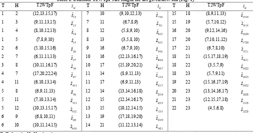
In Example 5.1 and Example 5.2, we have considered a real-life problem of a distribution network for a soft drink company. Here we consider a soft drink company which is having 23 distribution areas. This configuration is shown in Fig. 1. Now we can assume that the distance between the two distribution centres is a WTpFN where the arc length is given in Tables I and Table II. The company wants to find the SP for distribution between the geographical centres.

Railway Network:

In Example 5.3 and Example 5.4, we have considered a real-life situation of Railway

(4)

[image:4.595.322.519.112.246.2]

different railway stations. This configuration is shown in Fig. 2. Now we can assume that the distance between the two railway stations is a WTrFN where the arc length is given in Table III and Table IV. The railway authority wants to find the SP between the considered railway stations.

Here, we will test our method for the above-discussed problems where considered in [16,23,25,34]

Fig 1:The network contains 1 as a source and 23 as

a destination node. [21] Fig 2:and 5 as a destination node. [24-25] The network contains 1 as a source

Example 5. 1: Consider all the arc length is in T2WTpFN with the conditions of Table 1. Here, we consider a network see Fig 1.

Solution: After performing the steps 1-6, we getx151,

511 1

x  ,x₁₁₁₇1,x₁₇₂₁1, x₂₁₂₃1, rest allx_ij0. Hence

[image:4.595.67.292.117.244.2]

the SP is1 5 11 17 2123.now, put the value of all x_ij in Equation 5 then we get the FSP length as: (38, 49, 58, 65). So, we conclude that the FSP length lies within the range of 38 to 65. Moreover, the maximum possibility of the CSP length lies in between the range of 49 to 58. Additionally, our advanced method predicts the CSP is 52.50.

Table I:Consider T2WTpF Arc length for the given network (Fig. 1)

T H T2WTpF _s__kl T H T2WTpF __s_kl T H T2WTpF _s__kl

1 2 (12,13,15,17)

12

s

 7 10 (9,10,12,13)

710

s

 15 18 (8,9,11,13)

1518

s



1 3 (9,11,13,15)

13

s

 7 11 (6,7,8,9)

711

s

 15 19 (5,7,10,12)

1519

s



1 4 (8,10,12,13)

14

s

 8 12 (5,8,9,10)

812

s

 16 20 (9,12,14,16)

1620

s



1 5 (7,8,9,10)

15

s

 8 13 (3,5,8,10)

813

s

 17 20 (7,10,11,12)

1720

s



2 6 (5,10,15,16)

26

s

 9 16 (6,7,9,10)

916

s

 17 21 (6,7,8,10)

1721

s



2 7 (6,11,11,13)

27

s

 10 16 (12,13,16,17)

1016

s

 18 21 (15,17,18,19)

1821

s



3 8 (10,11,16,17)

38

s

 10 17 (15,19,20,21)

1017

s

 18 22 (3,5,7,9)

1822

s



4 7 (17,20,22,24)

47

s

 11 14 (8,9,11,13)

1114

s

 18 23 (5,7,9,11)

1823

s



4 11 (6,10,13,14)

411

s

 11 17 (6,9,11,13)

1117

s

 19 22 (15,16,17,19)

1922

s



5 8 (6,9,11,13)

58

s

 12 14 (13,14,16,18)

1214

s

 20 23 (13,14,16,17)

2023

s



5 11 (7,10,13,14)

511

s

 12 15 (12,14,16,17)

1215

s

 21 23 (12,15,17,18)

2123

s



5 12 (10,13,15,17)

512

s

 13 15 (10,12,14,15)

1315

s

 22 23 (4,5,6,8)

2223

s



6 9 (6,8,10,11)

69

s

 13 19 (17,18,19,20)

1319

s



6 10 (10,11,14,15)

610

s

 14 21 (11,12,13,14)

1421

s



T: Tail node, H: Head node.

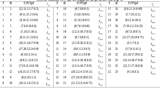
Example 5.2: Consider all the FAL is in T1WTpFN with the same network as mentioned in Example 5.1 and the cond. of Table II. Here, we consider a network see Fig 1.

Solution: After performing the steps 1-6, we getx121,

27 1

x  ,x₇₁₀1,x₁₀₁₇1, x₁₇₂₀1,x₂₀₂₃1 rest all are zero, i.e., xij0.

Hence the FSP is1 2  7 10 17 2023; now put the value of all xij in Equation 7 then we get the FSP

[image:4.595.47.553.403.669.2]

(5)

[image:5.595.43.564.58.339.2]

Table II:Consider T1WTpF arc length for the given network (Fig. 1)

T H T1WTpF

kl s

 T H T1WTpF

kl s

 T H T1WTpF

kl s

 1 2 (12,13,15,17;0.2)

12

s

 7 10 (6,7,8,9;0.3)

710

s

 15 18 (8,9,11,13;0.90)

1518

s



1 3 (9,11,13,15;0.4)

13

s

 7 11 (5,8,9,10;0.4)

711

s

 15 19 (5,7,10,12;1)

1519

s



1 4 (8,10,12,13;0.6)

14

s

 8 12 (3,5,8,10;0.5)

812

s

 16 20 (9,12,14,16;1)

1620

s



1 5 (7,8,9,10;0.8)

15

s

 8 13 (6,7,9,10;0.6)

813

s

 17 20 (7,10,11,12;0.25)

1720

s



2 6 (5,10,15,16;1)

26

s

 9 16 (12,13,16,17;0.8)

916

s

 17 21 (6,7,8,10;0.5)

1721

s



2 7 (6,11,11,13;0.3)

27

s

 10 16 (6,7,8,9;0.3)

1016

s

 18 21 (15,17,18,19;0.75)

1821

s



3 8 (10,11,16,17;0.6)

38

s

 10 17 (15,19,20,21;0.2)

1017

s

 18 22 (3,5,7,9;1)

1822

s



4 7 (17,20,22,24;0.9)

47

s

 11 14 (8,9,11,13;0.5)

1114

s

 18 23 (5,7,9,11;0.1)

1823

s



4 11 (6,10,13,14;1)

411

s

 11 17 (6,9,11,13;0.6)

1117

s

 19 22 (15,16,17,19;0.2)

1922

s



5 8 (6,9,11,13;0.25)

58

s

 12 14 (13,14,16,18;0.8)

1214

s

 20 23 (13,14,16,17;0.6)

2023

s



5 11 (7,10,13,14;0.50)

511

s

 12 15 (12,14,16,17;0.9)

1215

s

 21 23 (12,15,17,18;0.8)

2123

s



5 12 (10,13,15,17;0.75)

512

s

 13 15 (10,12,14,15;0.11)

1315

s

 22 23 (4,5,6,8;1)

2223

s



6 9 (6,8,10,11;1)

69

s

 13 19 (17,18,19,20;0.25)

1319

s



6 10 (10,11,14,15;0.1)

610

s

 14 21 (11,12,13,14;0.75)

1421

s



Example 5.3: Consider all the FAL is in T2WTpFN

[image:5.595.43.557.405.592.2]

with the same network as mentioned in Example 5.3 and the conditions of Table III. Here, we consider a network see Fig. 2 [23].

Table III:Consider T2WTrF arc length for the given network (Fig. 2)

T H T2WTrF s_kl T H T2WTrF s_kl T H T2WTrF s_kl

1 2 (800,820,840)

12

s

 3 5 (730,748,770)

35

s

 8 4 (710,730,735)

84

s



1 3 (350,361,370)

13

s

 3 8 (425,443,465)

38

s

 8 7 (230,242,255)

87

s



1 6 (650,677,683)

16

s

 4 5 (190,199,210)

45

s

 9 7 (120,130,150)

97

s



1 9 (290,300,350)

19

s

 4 6 (310,340,360)

46

s

 9 8 (130,137,145)

98

s



2 10 (420,450,470)

210

s

 4 11 (710,740,770)

411

s

 9 10 (230,242,260)

910

s



2 3 (180,186,193)

23

s

 5 6 (610,660,690)

56

s

 10 7 (330,342,350)

107

s



2 5 (495,510,525)

25

s

 6 11 (230,242,260)

611

s

 10 11 (1250,1310,1440)

1011

s



2 9 (900,930,960)

29

s

 7 6 (390,410,440)

76

s



3 4 (650,667,883)

34

s

 7 11 (450,472,490)

711

s



Solution: After performing the steps 1-6, we get x₁₃1,

35 1

x  rest allxij0.Hence, the FSP is 1 3 5; Now put the value of all

x

_ij in Equation 8 then we get and the FSP length as: (1080, 1109, 1140). So, we conclude that the FSP

length lies within the range of 1080 to 1140 and the maximum possibility of the CSP length is 1109. Moreover, ouradvanced method predicts the CSP is 1109.5.

Example 5.4: Consider Fig. 2 with the conditions of Table IV

Table IV: T1WTrFN with different membership function for Example 5.4 (fig. 2)

kl s

 T1WTrFN s_kl T1WTrFN s_kl T1WTrFN

12

s

 (800,820,840;0.1) _s_₃₅ (730,748,770;0.75) _s_₈₄ (710,730,735;1)

13

s

[image:5.595.39.564.693.839.2]

(6)

16

s

 (650,677,683;0.2) _s₄₅ (190,199,210;0.20) _s₉₇ (120,130,150;0.6)

19

s

 (290,300,350;0.9) _s₄₆ (310,340,360;0.40) _s₉₈ (130,137,145;0.9)

210

s

 (420,450,470;0.1) _s₄₁₁ (710,740,770;1) _s₉₁₀ (230,242,260;1)

23

s

 (180,186,193;0.2) _s_₅₆ (610,660,690;1) __s₁₀₇ (330,342,350;0.25)

25

s

 (495,510,525;0.3) __s₆₁₁ (230,242,260;0.2) _s_₁₀₁₁ (1250,1310,1440;0.5)

29

s

 (900,930,960;0.25) _s₇₆ (390,410,440;0.6)

34

s

 (650,667,883;0.50) _s₇₁₁ (450,472,490;0.8)

Solution: After performing the steps 1-6, we get x₁₂1,

25 1

x  rest allxij0. Hence the FSP is 1 2 5. Now put the value of all x_ij in Equation 10 we get the FSP length as: (1295, 1330, 1365; 0.1). Moreover, our advanced method predicts the CSP length is 1330.

VI. RESULTANDDISCUSSION

The result obtained from Example 5.1 for FSP length and FSP are (38, 49, 58, 65) and1 5 11 17   21 23 , respectively which is precisely the same as shown in [17,19,31,34]. We have already discussed the flaws of the

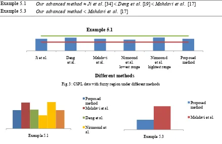
existing method of [17, 19], however, in our proposed method we overcome those flaws. Further, in Example 5.3 the FSP length and the FSP are obtained as (1080, 1109, 1140) and 1 3 5 which is precisely the same as shown in [17]. However, our proposed methods consume less space and computations and last but not the least, no complexity which helps a newcomer to understand. Moving further, the proposed method has been tested for both the above discussed Example 5.1 and Example 5.3 which have been already examined by many researchers. When our method has been compared (in Table V and Fig. 3-5) with the other existing methods, we can clearly observe that the CSPL is smaller than or equal to other discussed methods. In Table VI, we compare the objective value of the related techniques.

Table V:Logical comparative analysis with current methods.

Example 5.1 Our advanced method Ji et al≈ . [34]<Deng et al . [19]<Mahdavi et al . [17] Example 5.3 Our advanced method Mahdavi et al< . [17]

[image:6.595.46.540.60.189.2]

Fig. 3: CSPL data with fuzzy region under different methods

Fig 4: Objective value vs. existing method Fig. 5: Objective value vs. existing method

From Fig 3, Fig 4 and Fig 5, we can conclude that the objective value for all methods always lies within the fuzzy range.

To the best of our information, Example 5.2 and Example 5.4 are not taken into consideration by any researcher till date. We have discussed these problems as they are also the

applications of fuzzy weighted SPP. In Example 5.2, the FSPL and the FSP are obtained as (62, 77, 85, 93; 0.2) and 1 2  7 10 17 2023. In Example 5.4, FSPL and the FSP are obtained as

(1295, 1330, 1365; 0.1) and 1 2 5 . The proposed method not only works Ji et al. Deng

et al. Mahdavi et al. Nirmoond et al. lowest range

Nirmoond et al. hightest range

Proposed method

Different methods Example 5.1

Example 5.1

Proposed method Mahdavi et al.

Deng et al.

Nirmoond et al.

Example 5.3

Proposed method

[image:6.595.51.490.398.683.2]

(7)

under weighted trapezoidal fuzzy environment but also applicable under weighted triangular fuzzy environment. However, most of the current methods are either solved as Type-II weighted triangular fuzzy set problems or Type-II weighted trapezoidal fuzzy set problems; very few methods exist which works in both the environment. Furthermore, the proposed method works in both environments without any

[image:7.595.41.562.157.420.2]

limitation. So, due to this advantage, we overcome the limitation mentioned in Section 4.1. Also, we have concluded that our method is more reliable than any of the current methods. Table VI, clearly shows that the reliability of our advance method when compared to any of the current methods.

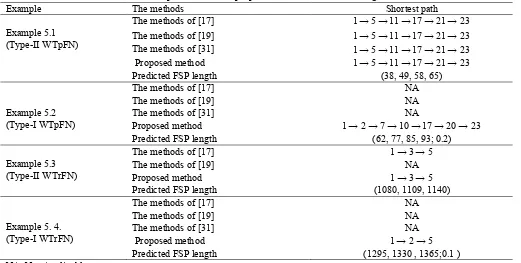
Table IV: Comparison with our proposed model with some existing models

Example The methods Shortest path

Example 5.1 (Type-II WTpFN)

The methods of [17] 1 5 11 17   21 23

The methods of [19] 1 5 11 17   21 23

The methods of [31] 1 5 11 17   21 23

Proposed method 1 5 11 17   21 23

Predicted FSP length (38, 49, 58, 65)

Example 5.2 (Type-I WTpFN)

The methods of [17] NA

Proposed method 1 2  7 10 17 2023

Predicted FSP length (62, 77, 85, 93; 0.2)

Example 5.3 (Type-II WTrFN)

The methods of [17] 1 3 5

Proposed method 1 3 5

Predicted FSP length (1080, 1109, 1140)

Example 5. 4. (Type-I WTrFN)

Proposed method 1 2 5

Predicted FSP length (1295, 1330 , 1365;0.1 )

NA: Not Applicable

VII. ADVANTAGESOFTHEPROPOSEDMODEL

i) We can easily find out the FSP and the FSPL.

ii) This algorithm uses some elementary idea of a scoring index and FLP theory which is easy for implementations.

iii) The vast knowledge of FLP is not required.

iv) The proposed method has an added advantage of solving the problems where arc lengths have varied weight.

v) The ultimate advantage of the advance algorithm is to solve a new set of a problem apart from the existing problems.

vi) This algorithm can predict the CSP length.

VIII. CONCLUSION

The proposed paper present a novel method to solve the Type-I and Type-II WTpFN and WTrFN. This method is capable of finding FSP, FSP length and also able to predict CSP length. Moreover, it reflects that our advanced method reduce the time, effort and space complexity over the current methods. From the numerical and graphical results, we can explain that the new novel method can solve different types of problems which can't be addressed by any of the existing methods. In future, we extend this single objective WTpFN and WTrFN method in bi-objective and multi objective environment.

REFERENCES

1. E. W. Dijkstra. (1959). A note on two problems in connexion with graphs. Numerische Mathematik. 1. 269-271.

2. R. W. Floyd. (1962). Algorithm 97: Shortest path. Commun. ACM. 5. 345

3. L. A. Zadeh. (1965). Fuzzy sets. Information and Control. 8. 338-353. 4. K. Nip, Z. Wang, and W. Xing. (2016). A study on several combination problems of classic shop scheduling and shortest path. Theor. Comput. Science. 654. 175-187.

5. K. Nachtigall. (1995). Time depending shortest-path problems with applications to railway networks. European Journal of Operational Research. 83. 154-166.

6. P. Crescenzi, P. Fraigniaud, M M Halldórsson, H A Harutyunyan, C Pierucci, A Pietracaprina, G Pucci. (2016). On the complexity of the shortest-path broadcast problem. Discrete Applied Mathematics. 199. 101-109.

7. D. Dubois and H. Prade. (1983). Ranking fuzzy numbers in the setting of possibility theory. Information Sciences. 30. 183-224.

8. Y. Li, M. Gen, and K. Ida. (1996). Solving fuzzy shortest path problems by neural networks. Computers & Industrial Engineering. 31. 861-865. 9. Y. Zhang, Z. Zhang, Y. Deng, and S. Mahadevan. (2013). A biologic

-ally inspired solution for fuzzy shortest path problems. Appl. Soft Computing. 13. 2356-2363.

(8)

11. A. Kaufmann and M. M. Gupta. (1985). Introduction to fuzzy arithm -etic: theory and applications. Von nostrand Reinhold Company.

12. T-N. Chuang and J-Y. Kung. (2005). The fuzzy shortest path length and the corresponding shortest path in a network. Computers & Operations Research. 32. 1409-1428.

13. R. Jain. (1976). Decision making in the presence of fuzzy variables.

IEEE Transactions on Systems, Man, and Cybernetics. 6. 698-703. 14. S-J. Chen and S-M. Chen. (2007). Fuzzy risk analysis based on the

ranking of generalized trapezoidal fuzzy numbers. Appl. Intell. 26. 1 -11. 15. C-H. Cheng. (1998). A new approach for ranking fuzzy numbers by

distance method. Fuzzy Sets and Systems. 95. 307-317.

16. S. A. Düzce. (2015). A new ranking method for trapezial fuzzy num -bers and its application to fuzzy risk analysis. Journal of Intelligent and Fuzzy Systems. 28. 1411-1419.

17. I. Mahdavi, R. Nourifar, A. Heidarzade, and N. Mahdavi-Amiri. (2009). A dynamic programming approach for finding shortest chains in a fuzzy network. Appl. Soft Computing. 9. 503-511.

18. E. Keshavarz and E. Khorram. (2009). A fuzzy shortest path with the highest reliability. Journal of Computational and Applied Mathematics. 230. 204-212.

19. Y. Deng, Y. Chen, Y. Zhang and S. Mahadevan. (2012). Fuzzy Dijkstra algorithm for shortest path problem under uncertain environment. Appl. Soft Computing. 12. 1231-1237.

20. S. Mukherjee. (2012). Dijkstra's algorithm for solving the shortest path problem on networks under intuitionistic fuzzy environment. Journal of Mathematical Modelling and Algorithms. 11. 345-359.

21. R Kumar, S Jha, and R Singh. (forthcoming). A different appraoch for solving the shortest path problem under mixed fuzzy environment.

International journal of fuzzy system applications. 9(2) Article 6. 22. R Kumar, S A Edalatpanah, S Jha, S Broumi, and A Dey. (2018).

Neutrosophic shortest path problem. Neutrosophic Sets and Systems. 23. 5-15.

23. R Kumar, S. Jha, and R. Singh. (2017). Shortest path problem in network with type-2 triangular fuzzy arc length. Journal of Applied Research on Industrial Engineering. 4. 1-7.

24. R Kumar, S A Edalatpanah, S. Jha, and R Singh. (2019). A novel approach to solve gaussian valued neutrosophic shortest path problems.

International Journal of Engineering and Advanced Technology. 8(3). 347-353.

25. R Kumar, S A Edalatpanah, S. Broumi S. Jha, R. Singh, and A. Dey. (2019). A multi objective programming approaches to solve integer valued neutrosophic shortest path problems. Neutrosophic Sets and Systems. 24. 134-149.

26. H.-J. Zimmermann. (1978). "Fuzzy programming and linear program -ming with several objective functions," Fuzzy Sets and Syste -ms, vol. 1, pp. 45-55.

27. H. R. Maleki, M. Tata, and M. Mashinchi. (2000). Linear programming with fuzzy variables. Fuzzy Sets and Systems. 109. 21-33.

28. H. S. Najafi and S. A. Edalatpanah. (2013). A note on “A new method for solving fully fuzzy linear programming problems”. Applied Mathem -atical Modelling. 37. 7865-7867.

29. A. Hosseinzadeh and S. A. Edalatpanah. (2016). A New Approach for Solving Fully Fuzzy Linear Programming by Using the Lexicography Method. Adv. Fuzzy Systems. 2016. 1538496:1--1538496:6

30. S. Mukherjee. (2015). Fuzzy programming technique for solving the shortest path problem on networks under triangular and trapezoidal fuzzy environment. International Journal of Mathematics in Operational Research. 7. 576-594.

31. S. Niroomand, A. Mahmoodirad, A. Heydari, F. Kardani, and A. Hadi –Vencheh. (2017). An extension principle based solution approach for shortest path problem with fuzzy arc lengths. Operational Research. 17. 395-411.

32. M. S. Bazaraa, J. J. Jarvis, and H. D.Sherali. (2010). Linear Program -ming and Network Flows, fourth Edition. A John Wiley & Sons, Inc., Publication.

33. S. Okada and T. Soper. (2000). A shortest path problem on a network with fuzzy arc lengths. Fuzzy Sets and Systems. 109. 129—140 34. X. Ji, K. Iwamura and Z. Shao. (2007). New models for shortest path

problem with fuzzy arc lengths. Applied Mathematical Modelling. 31(2). 259-269.

AUTHORS PROFILE

Ranjan Kumar, Research Scholar, National Institute of Technology, Jamshedpur. His fields of interest are uncertainty theory, Fuzzy Optimization and Operational Research.

Dr. S A Edalatpanah, Received his PhD in applied mathematics from the University of Guilan, Rasht, Iran. He is an academic member of Guilan University, Islamic Azad University, and Ayandegan Institute of Higher Education. His fields of interest are numerical linear algebra, soft computing and optimization. He is Editor-in-Chief of the International Journal of Research in Industrial Engineering at

www.riejournal.com.

Dr. Sripati Jha, Associate Proffesor, National Institute of Technology, Jamshedpur. His fields of interest are Fuzzy, Fuzzy Optimization and Operational Research. He is serving as Dean Alumni & Industrial Relations which is highly respectable administrative position in the institution. He has also served as Dean Student Welfare in the past.

Sudipta Gayen is a Research Scholar in Department of Mathematics, National Institute of Technology, Jamshedpur, India. His areas of interest areUncertainty theory, Fuzzy Optimization, Operational Research, Fuzzy Abstract algebra and its applications, Neutrosophic Abstract algebra and its applications.