Abstract: Border Gateway Protocol (BGP) is a vital protocol on the internet for transfer of data packets among Autonomous System (AS). Security is a major concern for the transmission of BGP packets which are often attacked by worms or are hijacked by an attacker which results in requests entering black holes or loss of connection to the particular sites. The BGP anomalies can be reduced by analyzing the BGP datasets. Since, ASes communicate through messages, therefore, the anomalies can be reduced by identifying the corrupted BGP message in the dataset. In this paper, BGP anomalies have been classified by applying Machine learning (ML) algorithms. The dataset contains information about the sending and receiving time between ASes. The classifiers were used to predict the anomalies. Since the dataset had high dimensions, the dimensions were reduced using Linear Discriminant Analysis (LDA) and then Support Vector Machines (SVM), K-Nearest Neighbors (KNN), Linear Regression, Logistic Regression and Multi-Layer Perceptron (MLP) have been used to classify the anomalies.
Keywords: Anomalies, BGP, Linear Discriminant Analysis, Machine Learning
I. INTRODUCTION
A
dynamic routing protocol defines the path selected between two routers for the communication. Border Gateway Protocol (BGP) is the protocol that is used to share routing information between different Internet Service Providers (ISPs).In BGP, information in the form of packets is shared and transferred between different Autonomous Systems (ASes). AS consist of systems under the same administration. Each AS contains a routing table that contains information about the surrounding ASes. Whenever there is any update in the topology, notifications are send to all the ASes. Any error in the connection is also notified through notifications. There is thus no requirement of refreshing the entire routing table. The BGP peers inside the AS communicate using the Interior Border Gateway Protocol (iBGP). On the other hand, peers under different Ases connect through Exterior Border Gateway Protocol (eBGP). The BGP peers in the same AS are connected by internal links whereas two BGP speakers in
Revised Manuscript Received on September 05, 2019. * Correspondence Author
Namrata Majumdar, Amity School of Engineering and Technology, Amity University, Noida, India. Email: [email protected]
Anisha Bhatnagar, Amity School of Engineering and Technology, Amity University, Noida, India. Email: [email protected]
*Shipra Shukla, Amity School of Engineering and Technology, Amity University, Noida, India. Email: [email protected]
different AS are connected through external links.
BGP anomalies can be detected by analyzing the BGP dataset. The machine learning techniques such as Support Vector Machines (SVM), K-Nearest Neighbors (KNN), Linear Regression, Logistic Regression and Multi-Layer Perceptron (MLP) can be applied for the classification of anomalies which can be further reduced.
A BGP dataset has been used and Linear Discriminant Analysis (LDA) has been applied. LDA connects the data to a low dimensional space which is based on the summation of local LDAs and uses a KNN procedure. LDA is an excellent method that extracts a linear feature. LDA is based on Fisher’s Discriminant Analysis. Additionally, LDA has been used in pattern recognition, business intelligence and some classification problems [1]. After reprocessing of the dataset ML algorithms were applied such as SVM, KNN, Linear and Logistic Regression and the MLP.
The paper has been divided into following sections which give insight on the features, messages, anomalies of the BGP. Section 2 provides the brief description of BGP features and messages. Anomalies in BGP are of different types such as direct and deliberate, direct and not deliberate, indirect and hardware failures which have been described in Section 3. Section 4 describes the classifiers that can predict the anomalies. Section 5 presents the results obtained after applying the algorithm. Section 6 concludes the paper.
II. BORDER GATEWAY PROTOCOL
A. Features of BGP
BGP provides a way in which one or more ASes can connect, synchronize and thus communicate with each other. The path for next hop of an AS is mentioned by the BGP. Messages are sent between ASes to communicate with each other. The messages contain information about the destination path. BGP describes policies that are understood by the administrator. Transmission Control Protocol is used by the BGP to communicate and thus is reliable. Complete information is only send once in BGP packet transfer. After that only update information called deltas are sent. BGP accepts classless addressing and always reviews the message and checks that the sender is a valid sender which means it adds security to the communication.
Using Linear Discriminant Analysis for
Dimensionality Reduction for Predicting
Anomalies of BGP data
B. BGP Messages
The information about the packets sent and received over the network for communication is exchanged in the form of messages. There are four types of messages used in BGP. The first one is the OPEN message. After building a connection between two ASes, the first message send by an AS is the OPEN message. Once the AS on the other side of the network receives the OPEN message then the latter sends a KEEPALIVE message as a confirmation that the connection has been established between the two. After this, except the OPEN messages, any other messages can be sent and received by the ASes. The second type of messages sent are the UPDATE messages that are used to share routing information between two ASes. Whenever there is a change in topology in a network then UPDATE messages are sent to update the topology. If there is an error in a connection then these UPDATE messages can be sent to inform the AS about the same and get it fixed. UPDATE messages are also sent when there is any need to delete certain routes. The third type of messages is the KEEPALIVE messages. This message is sent before the hold timer expires. It is sent in the time interval of one third time of hold time. It is used to keep the connection between two ASes alive. The NOTIFICATION messages are the last type of messages. This message is sent whenever there is an error in the connection. After this message the connection is cut off [2], [3].
III. BGP ANOMALIES
Since there are continuous paths that are being added to the topology, there is always a possibility that certain paths that are not secure gets added to the routing table. This leads to formation of anomalies. As UPDATE messages are sent every time there is any change in the topology, therefore, differentiating the update messages which may be anomaly based from those which are not is the real task that’s need to be taken care of. An update is classified as invalid only if it has an invalid AS number, has prefixes that are either already taken or are not valid or is announced by some AS which is not secure enough or if the AS_PATH mentioned does not exists [18]. There are four types of anomalies.
Direct and deliberate anomalies are caused due to hijacking such as prefix and suffix hijacking. This happens when a hijacker claims a prefix that belongs to some other AS as its own. This leads to all the data packets directing towards the hijacker. Like this, black holes are created where all the routes are diverted and thus are restricted from being used elsewhere. Another way, the attacker attacks is by staying in the middle and thus not directly stopping the traffic but delaying the data flow rate. Similarly, some false suffix can be advertised so that the attacker is able to redirect the traffic towards a particular site. False routing update messages and adding more number of hosts on the network causes aggregation on the link and thus creates an anomaly. For example in 2005 AS174 hijacked one of Google’s prefixes therefore it lost its connection with the site for nearly one hour. Also, AS12812 was hijacked in April 2011 for around 6 months. Direct and not deliberate anomalies are second type of anomalies. Faulty structure of an AS can lead to building of
AS always announces the prefixes it has used, this also gives a way to the hijackers to use those prefixes and cause discrepancies such as black holes or cause an overloading on an AS. This type of anomaly is different from the earlier one by the fact that after the operator detects a false prefix in use it stops the connections with the AS but during the process, anomalies such as packet loss, un-deliberate paths, etc. are possible. Pakistan in 2008 shared an invalid link to YouTube prefix which led many AS to loose connection with the site. Indosat also in 2014 showed 320,000 invalid routes.
Anomalies can be Indirect Anomalies. These are aimed towards the web servers. Worm attacks such as Nimda, Code Red II and Slammer attacks are in these kinds of anomalies. In 2001 the Nimda anomaly was detected where there was a 30 times increase in update messages. Also in 2003 Slammer anomaly was detected where there was huge increment in the number of update anomalies. Slammer is one of the fastest worm attacks. It attacks 90% hosts that are most likely to get attacked in about 10 minutes. Worms not only affect the end points of the network but also affect the overall structure of the BGP network. The worms reside at one particular end point and replicate themselves. On analyzing the BGP update messages of July 1 to September 24, 2001. It was found that two worms Code Red II and Nimda increased advertisement rate for several hours which does not take place in any local network failure. The attacks resulted in overload of router CPU, exhausted the memory and generated software routed bugs [4].
Anomalies can also be caused by hardware failures. This was observed when in 2005 there was a blackout in Moscow for many hours due the hardware failure. It affected many cities of Russia as well. The internet services were shut down for several hours. There has been failure of BGP services due to failing of Mediterranean cables in 2008. More than 20 countries were not reachable for several hours.
There are many approaches which have earlier been studied to help remove these anomalies:
1. S-BGP Architecture: It has three security solutions: Public Key Infrastructure (PKI) which can be used for authentication, Digital Signals which can be used in place of AS paths which were public and had a chance of getting attacked frequently and Data and partial sequence integrity is also a suggested solution [5].
2. Applying Cryptography is another solution. 3. Mitigation Approaches also helps for the same. 4. Detecting suspicious routes and then removing or
blocking them [6].
6. Minimum Redundancy Maximum Relevance (mRMR) feature selection has also been used in models to detect BGP anomalies and models of SVM and Long Short Term Memory (LSTM) were made [8].
7. Using Feature Selection algorithms such as Fisher and mRMR models of SVM and HMM (Hidden Markov Models) have been also designed with 86.1% and 84.4% accuracies [9].
Use of green BGP model which consists of two algorithms, in which one selects the appropriate path and the other works on energy saving using a model which reduces the power has been also been designed. This model helped to improve throughput upto 35%, the ratio of energy consumption increased upto 50% when compared to other techniques. The number of UPDATE messages exchanged was reduced to 71% and the convergence time required by the network reduced to 88% [10]. BGP convergence time has also been improved using MRAI timer which is adjustable [11].
IV. METHODOLOGY
ML is the ability of a machine to learn from experience and then to perform a task without being trained. It looks for some pattern and sequence in the data that is given to it and then trains itself so that it can perform in the same way in future on new data.
ML techniques have been used in calculating how accurately ML classifiers are able to predict the anomalies. ML is used to analyze a large amount of data at a faster rate and come up with useful and accurate solutions. The algorithms used are SVM, KNN, Linear Regression, Logistic Regression and MLP which have been explained in the paper [12].
A. SUPPORT VECTOR MACHINE
SVM is a supervised algorithm which is used for classification and regression analysis. It is a classifier which is able to draw clear distinctions in the graph in the form of a hyper plane. The 2D graph with the data points gets divided into two halves. Now any new data point coming in is going to fall on either of the one side according to its position in the graph. This classifier thus helps in finding the dividing line. For data that is linearly separable, there are two types of SVMs, hard margin and soft margin. For the dataset that is non-linear, kernel trick is used. The hyper plane is plotted using the kernel function. The aim of the algorithm is to maximize the margin. SVM is based on linear division method. In case of non-linear division method, the SVM converts and connects a low dimensional space point to the high dimensional space to make it suitable for linear division [13].
SVM uses structural risk minimization algorithm. It does not get effected from the dimensions of the feature space. It always works well no matter how many number of features are used. It is most commonly used for text categorization [14]. The following parameters affect the working of the classifiers.
1. kernel: It is used to derive relations or functions in case the data is nonlinear. The different kernels are linear kernel, rbf kernel, polynomial kernel and sigmoid kernel.
2. gamma: It gives information whether the points are at large or close proximity and whether it will influence the boundary line or not.
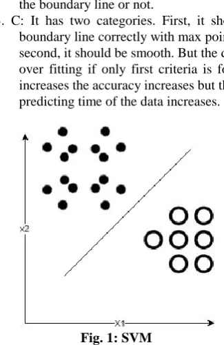
3. C: It has two categories. First, it should draw the boundary line correctly with max point covered and second, it should be smooth. But the data may cause over fitting if only first criteria is followed. As C increases the accuracy increases but the training and predicting time of the data increases.
Fig. 1: SVM
In fig. 1, the SVM algorithm has used two features x1 and x2 and then classified the dataset into two classes represented by black and white circles.
B. K-NEAREST NEIGHBORS
KNN is a supervised learning algorithm that trains the computer in recognizing similar objects. Therefore it helps to differentiate between different types of data. Thus after training the algorithm, the algorithm is now able to categorize/classify an unnamed data. The output labels are usually represented as numeric values such as 0, 1,-1etc. This numbers basically represents the categories of classification. The algorithm uses straight distance algorithm to group data points which are near each other and thus draws categories between them. One of the important steps in this algorithm is the choosing of parameter n_neighbor. n_neighbor should be chosen so that it gives minimum error. Weighted voting methods are also developed in KNN to get better results [15]. The algorithm depends on the value of n_neighbor we choose and the distance metric applied. It is easy to implement and can be used as a regression, classifier or can be also used as a searcher. The only disadvantage this algorithm faces is that it is quite slower than the other algorithms.
Parameters used in this classifier are as follows: 1. n_neighbors : This parameter chooses the number of
neighbors that will affect the prediction of test points.
[image:3.595.327.490.77.328.2]3. algorithm: This parameter gives achoice between the different algorithms as follows:
3.1.ball tree: It is efficient on data that has a complex structure.
3.2. kd tree: Distance calculations are reduced using this algorithm. It also reduces computation complexity but it is not efficient for data with higher dimensions.
3.3.brute: The brute force is the computation of distances between all pairs.
3.4.Auto: The machine tries to choose the best algorithm on its own
.
Fig. 2. KNN
In Fig. 2, there are two types of classes, ovals and diamonds. Any new data point, in this case the triangle can be classified in one of the classes by using KNN. Here the triangle will belong to the oval class as its distance from the oval class is less than the diamond class.
C. LINEAR REGRESSION
Linear Regression is also a part of supervised learning algorithm. It has one dependent and one independent variable. It trains the data to form a slope. The slope is made based on a cost function. The cost function used is a polynomial of any order. The cost function is built on the base of minimizing the squared distances. It has a continuous output variable which is a dependent variable. The output can have any value. The input variables can be one or more than one and are always independent. This algorithm uses minimum squared distance value to calculate the error. It has many applications, some of them are – it has been used to detect age of author from the text [16], multi variable linear regression has been used to predict the market value of footballers. The variables were the factors which affected the market values. The results gave 52 attributes which were used with %20 MAPE and 0.86 R^2 value after adjusting[17].
Parameters used are as follows:
1.fit_intercept: If it is set to true, then the intercept is calculated otherwise not.
2. n_jobs: It tells the classifier how many samples to use compute the slope.
3.normalize: The to-be regressed values will be normalized i.e. they will be subtracted from the maximum value and divided by the range before
[image:4.595.337.505.64.205.2]
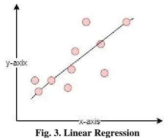
Fig. 3. Linear Regression
As in Fig. 3, a hypotenuse is drawn on the data points. The main objective of this algorithm is to reduce the distance of the points from the hypotenuse.
D. LOGISTIC REGRESSION
Logistic Regression is also a type of supervised learning algorithm. In this type of regression there is more than one dependent variable. The output has discrete values as it will answer yes or no for an event to be existing or not. The cost function is in exponential form. It uses sigmoid function to compute the cost. It has been using maximum livelihood method to find the error. The probalities in logistic regression should be between 0 to 1. The probabilities of all the objects add up to one. It has been used in many fields such as finding important variables for the traffic lights [18]. The independent variables have an effect on the result variables. This is calculated by the logistic regression classifier. Regularization applied to logistic regression can help in case where the data has a large number of features which usually causes over fitting.
Parameters used are as follows:
1. penalty: Used to specify the rule of penalization. 2. tol: It specifies the tolerating limit.
3. c: It works in the opposite way regularization works. 4. fit_intercept: It specifies the value of intercept of the
slope.
5. random_state: It generates the random state using the random number generator.
E. MULTI-LAYER PERCEPTRON
MLP stands for Multi-Layer Perceptron. There is more than one linear layer in MLP. The top layer is known as the input layer and the last layer is known as the output layer and all the layers in between these two layers are called the hidden layer. The performance of the algorithm is calculated by the function called the loss function. The weights are added to the random values and after each iteration, the aim is to need to reduce the loss.
Parameters used are as follows:
1.hidden_layer_sizes: The number of hidden layers between the input and the output layer is mentioned through this parameter.
2.activation: It mentions the activation function. 3.solver: The optimization technique used for
4.learning_rate: It is used to mention the learning rate.
5.random_state: The random state generator is used to generate the random state.
Scikit Learn Library, Mathplot Library and Pandas Library was used. Python 2 was used for writing the code. The dataset represents the difference in between the time a data packet is received and send further to the following AS. The dataset represents the hoping of a data packet from 109 ASes. It consists of 110 columns and 126101 rows. Using the different ML algorithms, classifiers were built using different parameters each time to reduce error and after training testing the following accuracies were obtained. Since the data is a multidimensional, there we should reduce it. Therefore we have used LDA.
LDA stands for Linear Discriminant Analysis. It is another type of supervised machine learning algorithm. It is used for reducing the dimension of the dataset. This algorithm reduces the dimension as desired by removing the features that are dependent on the other features. It also removes the data which appears more than once in the dataset. This algorithm is generally used before processing the data. The variance between the classes is first calculated. Then the distance between the sample in a class and mean is calculated. Then the last step is to build the dimensional space in which the variance increases and the distance between sample and mean of the class decreases to minimum value. The main role of this algorithm which sets this apart from others is that it uses Bayes Rule to add probabilities to the classes. It is very similar to Principal Component Analysis (PCA), the only difference is the aim in PCA is to maximize the variance but in this the aim is to maximize the separation between the classes. It has helped in reducing over fitting problems. This algorithm finds its application in the pattern recognizing genre. The algorithm is used in the field of biometrics, bioinformatics and many more.
Applying the LDA before applying all the supervised algorithms helps to calculate the different accuracies for the different supervised machine learning algorithms. The parameters are changed in the each of the algorithms and respective graphs are plotted to see how parameters affects the working of an algorithm.
V. RESULTS A. SUPPORT VECTOR MACHINE
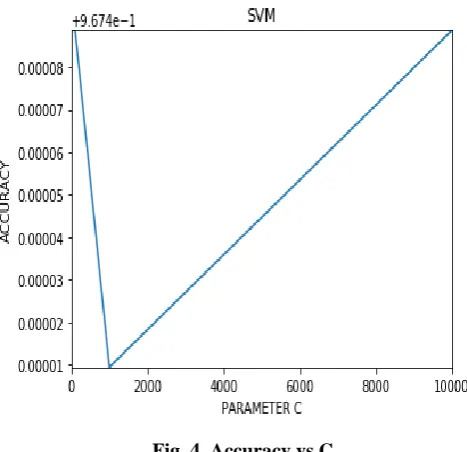
In this case the value of the parameter C has been changed to 10,100,1000,10000 and then accuracy has been calculated for each of the cases. The accuracies are mentioned in table I. Graph was plotted of parameter C vs the accuracy as given in Fig. 4. The accuracy first decreases and then starts increasing around C=1000. But the computational time also increases as the value of C increases. Therefore, a high value of C is not feasible.
Table I: SVM-Accuracies and Computational Time S.NO. C ACCURACY COMPUTATION TIME
1. 10 0.96748870034097
21
759.112
2. 100 0.96748870034097
21
2250.162
3. 1000 0.96740940448814
53
3235.87
4. 10000 0.96748870034097
21
4165.188
[image:5.595.305.539.58.284.2]
Fig. 4. Accuracy vs C
Therefore, appropriate value of C, which balances between the accuracy and computational time should be chosen. In this kernel=”linear” cannot be used as the data is nonlinear. B. K-NEAREST NEIGHBORS
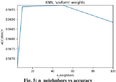
The values of n_neighbors have been changed and accuracies were calculated for weights being uniform and distance. The graphs were plotted in both the cases. First, the weights were kept ”uniform” and the values of n_neighbors were changed from 100 to 5 and accuracies and computational time were calculated as given in the table II.
Table II: KNN- Accuracies and Computational Time S.NO. N_NEIGH
BORS
ACCURACY COMPUTATIONAL
TIME
1. 100 0.9688367298390295 0.729
2. 50 0.9697089842201253 0.604
3. 10 0.9696296883672983 0.526
4. 5 0.9665371501070494 0.517
Fig. 5: n_neighnbors vs accuracy
In the second case the weights were fixed to distance and then the value of n_neighbors was changed from 100 to 5, and the accuracies and computational time were calculated similarly as the above case as given in the table III.
Table III: KNN-Accuracies and Computational Time S.NO. N_NEIGH
BORS
ACCURACIES COMPUTATIONAL
TIME
1. 100 0.9676472920466259 0.488
2. 50 0.966854333518357 0.365
3. 10 0.964554753786377 0.269
4. 5 0.9615415113789548 0.279
[image:6.595.307.567.262.389.2]n-neighbors vs accuracy was plotted as given in Fig. 6.
Fig. 6: n-neighbors vs accuracy The accuracy increases but there is a break in the slope at 2 points in the graphs. We need to use a large value for n_neighbors to gain high accuracy. So analyzing both the cases it can be concluded that the in case of uniform weigths low value for n_neighbors needs to be used, which is opposite from the case when distance weights is used, which gives high accuracy only when high values of n_neighbors is used.
C. LINEAR REGRESSION
Applying linear regression accuracy of 0.8568362890244233 along with regression coefficient of
0.4660202063792852 was obtained. The computational time of 0.03 was noted.
D. LOGISTIC REGRESSION
Applying logistic regression accuracy of 0.9647133454920308 along with regression coefficient of 1.756852180 and regression intercept of0.40407226 was obtained. The computational time of 0.179 was noted.
By comparing the accuracy between linear and logistic regression, it can be concluded that logistic regression gives much higher accuracy than linear regression with less computational time.
E. MULTI-LINEAR PERCEPTRON
By changing the value of hidden_layer_size from 500 to 10 and random_state set to 5, accuracy and the computational time was calculated as given in table IV.
Table IV: MLP-Accuracies and Computational Time S.N
O
HIDDEN_LAYER
_SIZES
ACCURACY COMPUTATION
AL TIME
1. 500 0.9671715169296646 138.528
2. 200 0.9671715169296646 66.897
3. 100 0.9674094044881453 78.139
4. 50 0.9671715169296646 46.777
5 10 0.965268416461819 10.289
[image:6.595.46.285.422.616.2]Hidden_layer_sizes vs accuracy was plotted as shown in Fig. 7.
Fig. 7: hidden_layer_sizes vs accuracy
The accuracy shows variance as hidden_layer_sizes are changed. The accuracy is constant between hidden_layer_size from 200 to 500. It increases rapidly in the beginning and is highest when hidden_layer_size is around 100. But computational time also increases as the size of hidden layer increases. Therefore, both the factors are needed to be analyzed before choosing the
[image:6.595.313.550.449.642.2]VI. CONCLUSION
SVMs gave an accuracy of 96.7488% but very high values of C increased the computational time. KNN with uniform weights gave an accuracy of 96.9708% while KNN with distance as weights gave an accuracy of 96.7647%. The computational time for uniform weights was very less compared to distance as weights. Linear Regression gives the lowest accuracy of 85.6836%. On the other hand, Logistic Regression gives accuracy of 96.4713%. The accuracy recorded for MLP was 96.7409%. Therefore, BGP anomalies can be identified with upto 96% correctness using these ML algorithms.
REFERENCES
1. Q. Li, F. Wei, and S. Zhou, “Local kernel nonparametric discriminant analysis for adaptive extraction of complex structures”, Open Physics, 15(1), 2017, pp. 270-279.
2. https://tools.ietf.org/html/rfc4271 3. https://tools.ietf.org/html/rfc1771
4. James Cowie, Andrew Ogielski, B. J. Premore, and Yougu Yuan, “Internet worms and global routing instabilities”, 2002.
5. S. Kent, C. Lynn and K. Seo, “Secure border gateway protocol (S-BGP)”, IEEE J. Sel. Areas Commun., vol. 18, no. 4, 2000, pp. 582–592,
6. B. Al-Musawi, P. Branch, and G. Armitage, “ BGP Anomaly Detection
Techniques: A Survey”, in IEEE Communications Surveys & Tutorials, vol. 19, no. 1, 2017, pp. 377-396.
7. Xianbo Dai, Na Wang and Wenjuan Wang, “Application of machine learning in BGP anomaly detection”. Journal of Physics: Conference Series, 2019.
8. Qingye Ding, Zhida, Li, P. Batta and L. Trajković, “Detecting BGP anomalies using machine learning techniques”, IEEE International Conference on Systems, Man, and Cybernetics (SMC), 2016, pp. 003352-003355.
9. N. M. Al-Rousan and L. Trajković, “Machine learning models for classification of BGP anomalies”, IEEE 13th International Conference on High Performance Switching and Routing, 2012, pp. 103-108. 10. S. Shukla and M. Kumar, “An Improved Energy Efficient Quality of
Service Routing for Border Gateway Protocol”, Computer and Electrical Engineering, Elsevier, Vol. 67, 2018.
11. S. Shukla and M. Kumar, “An Approach to Discover the Stable Routes in BGP Confederations”, International Journal of Information System Modeling and Design, Vol 8, Issue 2, 2018.
12. A. Bhatnagar, S. Shukla and N. Majumdar, “Machine Learning Techniques to Reduce Error in the Internet of Things”, 9th International Conference on Cloud Computing, Data Science & Engineering (Confluence), Noida, India, 2019, pp. 403-408. 13. Yujun Yang, Jianping Li and Yimei, Yang, “The research of the fast
SVM classifier method”, 12th International Computer Conference on Wavelet Active Media Technology and Information Processing (ICCWAMTIP), Chengdu, 2015, pp. 121-124.
14. T. Joachims, “Text categorization with Support Vector Machines:Learning with many relevant features”, In: Nédellec C., Rouveirol C. (eds) Machine Learning: ECML-98, ECML 1998. Lecture Notes in Computer Science (Lecture Notes in Artificial Intelligence), vol 1398.
15. G. Eason, B. Noble, and I.N. Sneddon, “On certain integrals of Lipschitz-Hankel type involving products of Bessel functions,” Phil. Trans. Roy. Soc. London, vol. A247, pp. 529-551, April 1955. 16. S. B. Imandoust & M. Bolandraftar, “Application of K-Nearest
Neighbor (KNN) Approach for Predicting Economic Events: Theoretical Background”, 2013.
17. Dong Nguyen, Noah A. Smith and Carolyn P. Ros´e, “Author Age Prediction from Text using Linear Regression” LaTeCH’11 Proceedings of the 5th ACL-HLT Workshop on Language Technology for Cultural Heritage, Social Sciences, and Humanities, 2011, pp. 115-123.
18. S. Shukla and M. Kumar,“Improving Convergence in iBGP Route Reflectors”, Advances in Electronics, Communication and Computing. Lecture Notes in Electrical Engineering, vol 443, 2018, pp. 381-388.
19. Layla A. Ahmed “Using logistic regression in determining the effective variables in traffic accidents.” Applied Mathematical Sciences, Vol. 11, 2017, no. 42, pp. 2047-2058.
AUTHORS PROFILE
Namrata Majumdar is currently pursuing B.Tech degree in Computer Science and Engineering. Her current research interests include Machine Learning, Iot and routing in the internet.
Anisha Bhatnagar is currently pursuing B.Tech degree in Computer Science and Engineering. Her current research interests are Machine Learning, Deep Learning, IoT and routing in the internet.