Stability analysis tool for tuning unconstrained decentralized model predicitive controllers

STABILITY ANALYSIS TOOL FOR TUNING

UNCONSTRAINED DECENTRALIZED MODEL PREDICTIVE CONTROLLERS

Massimo Vaccarini∗Sauro Longhi∗M. Reza Katebi∗∗

∗_{D.I.I.G.A., Universit`a Politecnica delle Marche, Ancona, Italy} ∗∗_{Industrial Control Centre, University of Strathclyde, Glasgow,}

Scotland, UK

Abstract: Some processes are naturally suitable to be controlled in a decentralized framework: centralized control solutions are often infeasible in dealing with large scale plants and they are technologically prohibitive when the processes are too fast for the available computational resources. In these cases, the resulting control problem is usually split in many smaller subproblems and the global requirements are guaranteed by means of a proper coordination. The unconstrained decentralized case is here considered and a coordination strategy is proposed for improving the global control performances. This paper present a tool for setting up and tuning a nominally stable decentralized Model Predictive Controller. Numerical examples are proposed for testing and validating the developed technique.

Keywords: Decentralized Control, Predictive Control, Communication Networks, Stability Analysis, Optimal Regulators

1. INTRODUCTION

The current diffusion of networks allows the control technologies and methodologies to fully express their potentials in many application fields. By means of the fast communication technologies, nowadays different independent controllers distributed in a wide area can exchange information in order to improve both the local and the global control performances. Robotic ap-plications with multiple autonomous agents pursuing a common goal, control applications in manufacturing and process industry where multiple units coopera-tively make a product, supply chains in which multiple actors that influence each other are involved, and large scale power systems represent some typical situations.

A decentralized control solution based on independent agents is here considered for the regulation of dif-ferent interacting processes. Global objectives, such as closed-loop stability and performance requirements for the global process require coordination among the control agents.

A partitioning of both actuators and sensors has been proposed by Motee and Sayyar-Rodsari (2003) as a solution for the problem of computational complexity for the use of MPC technology in large scale dynamic systems. Adopting a proper decentralized solution, the global computational effort can be reduced without significant degradations of the control performances and the fault tolerant issues can be improved (El-Farra

et al., 2004).

The functionalities of a Networked Decentralized Model Predictive Control solution (ND-MPC) have been recently tested on real plants with relatively strong interactions. The results obtained with the de-centralized MPC of a gasifier seem to be satisfactory if compared with those obtained by the classical cen-tralized MPC (Longhi et al., 2005). Stability analysis tools for testing the stability of the ND-MPC archi-tecture have been also proposed by Vaccarini et al. (2006).

This paper summarizes the results on the stability analysis developed by the authors and present a set of simulation tests to validate the proposed tool and to illustrate its use for the synthesis of decentralized controllers with communication networks. After a de-scription of the adopted ND-MPC strategy provided in Section 2, the stability analysis tool is presented in Section 3. Based on the former considerations, the control algorithm is outlined in Section 4 and the tool is applied to the synthesis of decentralized controllers for a set of testing plants in Section 5.

In order to simplify the mathematical expressions, some notations are here introduced. Given the num-bers k∈Z, h∈Z, m∈N, j∈N, i∈N, n∈Nsuch that

k≥h, j≥1, m≥h−k+1, i=1, . . . ,n:

• kvkA,ATvA is the norm of vector v induced by

matrix A;

• λj{A} is the j-th eigenvalue of a square matrix

A.

• x(kˆ |h),E£x(k)¯¯Yh¤is the (h−k)-step ahead

prediction of x, given the measurementsYh up

to time k;

• u(k|h)is the value of u(k), computed at time h;

• Xi(k,m|h)is a stacked vector made by the vectors

xi(k|h), . . . ,xi(k+m−1|h);

• X(k,m|h)is a stacked vector made by the vectors

X1(k,m|h), . . . ,Xn(k,m|h);

2. NETWORKED DECENTRALIZED MPC

For achieving global performance objectives, a coor-dination scheme based on communication among con-trol agents is developed. The concon-trol actions are com-puted by a set of subcontrollers which are independent agents able to dynamically exchange a restricted set of information. In the proposed control architecture,

each agentAiimplements an MPC algorithm for the

subsystem Si using both local information acquired

onSiand the estimate of the interactions amongSi

and the other subsystemsSj, j=1, . . . ,n, j6=i. The

resulting optimal sequence and the future prediction of the state over the prediction horizon, have to be exchanged among subsystems through a Local Area Network (LAN).

As well known, Model Predictive Control acts accord-ing to the recedaccord-ing horizon principle: at each samplaccord-ing time, using a predictive model of the system dynamics, the response of the process to changes in manipulated variables over a fixed horizon is predicted. Based on a proper cost function, a finite-horizon optimal control problem is solved to obtain current and future moves of the manipulated variables. Only the first computed move is applied to the real system. The same pro-cedure is repeated at the next control step based on the new measurement. Although this computation is an open-loop control problem, the receding horizon principle allows MPC to generate a feedback-control law.

Let consider a linear, discrete-time representation of a

plantP:

x(k+1) =Ax(k) +Bu(k) (1a)

y(k) =Cx(k). (1b)

and denote with x∈Rnx_{, u}∈Rnu_{, y}(k)∈Rny _and

yd∈Rny_{, its state, control input, output and desired}

output, respectively. Suppose thatP is composed by

n subsystemsSiwhose state-space representation is:

xi(k+1) =Aiixi(k) +Biiui(k) +wi(k) (2a) yi(k) =Ciixi(k) +vi(k). (2b)

where vectors xii, ui, yiand ydi are the local state,

con-trol input, output and desired output respectively, and

vectors wi and vi, named state and output interaction

vectors, are given by:

vi(k), n

∑

j=1(j6=i)

Ai jxj(k) + n

∑

j=1(j6=i)

Bi juj(k), (3a)

wi(k), n

∑

j=1(j6=i)

Ci jxj(k). (3b)

Definition 1. (ND-MPC). Given the plant P

com-posed by n subsystems Si, i=1, . . . ,n the

uncon-strained Networked Decentralized Model Predictive Control problem with prediction horizon p and con-trol horizon m consists of finding, at time k, a set of independent agentsAi, i=1, . . . ,n, such that eachAi

minimizes the local cost function

Ji, p

∑

l=1 ° °

°yˆi(k+l|k)−yd_i(k+l|k)

° ° °

Qi

+

+ m

∑

l=1 ° °

°∆ui(k+l−1|k)

° ° °

Ri

, (4a)

ˆ

yi(k+l|k) =vˆi(k+l|k−1) +CiiAliixˆi(k|k)+ +

l

∑

s=1

CiiAs−ii 1Biiui(k+l−s|k)+

+ l

∑

s=1

CiiAs−ii 1wˆi(k+l−s|k−1). (4b)

Definition 2. (Interaction). When a changes in input,

state or output variables of a subsystemSi produces

variations of input, state or output variables of a sub-systemSj, it is said thatSiinteracts withSj. Definition 3. (Connection). When the agentAi sends

information about the future behavior of subsystemSi

to the agentAj, it is said thatAiis connected withAj. Definition 4. (Neighboring Agent). If the agentAi is

connected with Aj, Ai is called input neighboring

agent ofAjandAjis called output neighboring agent

ofAi.AiandAjare said neighboring agents.

Definition 5. (Neighborhood of an Agent). The input

(output) neighborhood of an agentAi is the set of its

input (output) neighboring agents.

Each agent Ai, solution to the ND-MPC problem,

can be decomposed in three parts: an optimizer, a state predictor and an interaction predictor. At time

k, based on the exchanged information, the

interac-tion predicinterac-tion together with the local measurement is used by the optimizer to solve the MPC optimiza-tion problem. Once computed the optimal sequence

{∆ui(k|k), . . . ,∆ui(k+m−1|k)}, which minimize the

cost function (4a), the first element∆ui(k|k)is selected

and ui(k) =ui(k−1) +∆ui(k|k)is applied as control

input to Si. Then the state predictor computes an

estimate of the future state trajectory and broadcasts the optimal control sequence over the control horizon and the state predictions over the prediction horizon to its output neighborhood.

The following assumptions are here considered:

Assumptions 1.

• prediction and control horizons are the same for

each agent;

• control agents are synchronous;

• control agents communicate only once within a

sampling interval;

• the communication channel introduces a delay of

a single sampling time.

Lemma 1. (Quadratic Program). Under the

Assump-tions 1, at step k, each agentAi solution to the

ND-MPC problem, has to solve the following optimization problem:

min

∆Ui(k,m|k)

Ji=∆Ui(k,m|k)THi∆Ui(k,m|k)−GTi∆Ui(k,m|k).

(5)

where

Hi=NiTQ¯iNi+R¯i, (6a) Gi=2NiTQ¯i[Yid(k+1,p|k)−Lixˆi(k|k)−Miui(k−1)+

−SiWˆi(k,p|k−1)−TiVˆi(k,p|k−1)]. (6b)

The introduced matrices are used for computing the output predictions: Li, Mi, Ni, Si depend only on the

system matrices Ai, Biand Ci, matrix Tiintroduces a

unit delay in the interaction vector and matrices ¯Qi, ¯Ri

are made by a block replication of the local weighting

matrices Qi, Ri. Equation (5) defines an unconstrained

Quadratic Program which has to be solved on-line at each sampling instant.

For the sake of brevity, all the proofs of the results stated in this paper are are omitted. Refer to Longhi

et al. (2005) and Vaccarini et al. (2006) for further

details.

3. STABILITY ANALYSIS OF ND-MPC

The main idea is to find an explicit solution for the ND-MPC problem and to use it for obtaining a math-ematical representation of the closed-loop system. Once the closed-loop dynamic is known, the stability condition can be verified by analyzing the dynamic matrix.

For this purpose, denote with ˜Ai, ˜Bi, ˜Ci, ¯Ai and ¯Bi

proper local interaction matrices and with ˜A, ˜B, ˜C,

¯

A and ¯B their corresponding global stacked versions.

The gain of each MPC agent for the control effort

movement is represented by Kiwhereas matrixκi

rep-resents the gain for the magnitude of the local control

effort over the whole control horizon m. Define I0as

the matrix for selecting the first computed movements

from the optimal control sequence. Denote with ¯Li,

¯

Mi two state prediction matrices composed by

sys-tem matrices, and introduce I_i0as an auxiliary identity

block matrix. Assume that L, M, ¯L, ¯M, S, T , I0,κ are diagonalizations of the local matrices Li, Mi, ¯Li, ¯Mi, Si, Ti, Ii0,κirespectively and define:

θ,−κL, φ,−κ¡S ˜A+T ˜C¢, (7a)

ρ,I0I0−κ¡MI0+S ˜B¢. (7b)

Lemma 2. (Interaction Predictor). Under the

Assump-tions 1, at step k, for each agent Ai solution to the

ND-MPC problem, the predictions of the interaction vectors are given by:

ˆ

Wi(k,p|k−1) =A˜iX(kˆ ,p|k−1) +B˜iU(k−1,m|k−1),

(8a) ˆ

Vi(k,p|k−1) =C˜iXˆ(k,p|k−1), (8b)

and the global prediction vectors take the following form:

ˆ

W(k,p|k−1) =A ˆ˜X(k,p|k−1) +BU˜ (k−1,m|k−1), (9a) ˆ

The stacked vectors X(k,p|h)and U(k−1,m|h) are built with both the local estimations and the informa-tion collected from the input neighborhood by agent

Ai. Null entries will correspond to the subsystems

which don’t belong to the input neighborhood. Note

that at time k, agentAiuses the predictions computed

and broadcasted at time k−1{vˆi(k|k−1), . . . ,vˆi(k+ p−1|k−1)}and{wˆi(k|k−1), . . . ,wˆi(k+p−1|k−1)}.

Lemma 3. (State Predictor). Under the Assumptions

1, at step k, for each agent Ai solution to the

ND-MPC problem, the decentralized state prediction for

the agentAiis expressed by:

ˆ

Xi(k+1,p|k) =¯Lixˆi(k|k) +M¯iUi(k,m|k)+ +_A¯

iXˆ(k,p|k−1) +B¯iU(k−1,m|k−1). (10)

and the decentralized prediction equation for the over-all system is given by the matrix form:

ˆ

X(k+1,p|k) =¯L ˆx(k|k) +_MU¯ _(k,m|k)+

+_{A ˆ}¯_{X(k,p|k−1) +BU(k}¯ _{−1,m|k−1). (11)}

Lemma 4. (Explicit Solution). Under the Assumptions

1, at step k, for each agentAisolution to the ND-MPC

problem, the explicit form of the control action applied

by the agentAito the subsystemSiis given by:

ui(k) = (I−KiMi)ui(k−1)+ +Ki

h

Y_id(k+1,p|k)−Lixˆi(k|k)

i

+

−KiSiWˆi(k,p|k−1)−KiTiVˆi(k,p|k−1). (12) Lemma 5. (Optimal Control Sequence). Under the

As-sumptions 1, at step k, for each agentAi solution to

the ND-MPC problem, the expression of the optimal control sequence Ui(k,m|k)is:

Ui(k,m|k) =Ii0ui(k−1)+

κi

h

Y_id(k+1,p|k)−Lixi(k)−Miui(k−1)+

−SiWˆi(k,p|k−1)−TiVˆi(k,p|k−1)

i

. (13)

and its global expression is:

U(k,m|k) = θx(kˆ |k) +φ_Xˆ_(k,p|k−1)

+ρU(k−1,m|k−1)+

+κYd(k+1,p|k). (14)

Theorem 1. (ND-MPC Stability).

The closed-loop system given by the feedback

connec-tion of the plantP with a solution of the ND-MPC

problem, composed by a set of independent agentsAi,

i=1, . . . ,n, is asymptotically stable if and only if:

¯ ¯ ¯ ¯ ¯ ¯ ¯ ¯

λj

   

   

  

A 0 BI0 0

¯L _A¯ _M¯ _B¯

θA+φ¯L φA¯ ρ+θBI0+φM¯ φB¯

0 0 Imnu 0



  

   

   ¯ ¯ ¯ ¯ ¯ ¯ ¯ ¯

<1,

∀j∈[1, . . . ,nND], nND=pnx+nx+2mnu, (15)

where the nND is the order of the global closed-loop

system.

The first two block rows of the global closed loop dy-namic matrix in Equation (15) are formed by elements of matrix A (in the first two block columns) and matrix B (in the remaining two block columns). The Third block row is made by all the process matrices A, B and

C and the weighting matrices Qi and Ri and depends

also on the horizons p and m.

4. CONTROL ALGORITHM

At sample time k, each agentAi, solution to the

ND-MPC problem:

(i) Acquires the measures.

(ii) Acquires the predicted future state trajectories

Xj(k,p|k−1)and control inputs Uj(k,m|k−1)

from the neighboring agents and, once com-bined with the local state trajectory Xi(k,p|k−

1)and the control input Ui(k,m|k−1), it builds X(k,p|k−1) and U(k,m|k−1) and computes the corresponding predictions of the interactions (8a).

(iii) Computes the optimal control sequence (13).

(iv) Applies the first element ui(k) =I0

iUi(k,m|k)of

the optimal sequence Ui(k,m|k)as control input

toSi.

(v) Computes the future state trajectory (10) of the

subsystem Si over the prediction horizon p

where ˆxi(k|k) =xi(k)is given by the measures.

(vi) Broadcasts the optimal sequence Ui(k,m|k)and

the predicted state trajectory Xi(k+1,p|k)to the

neighboring agents. (vii) Iterates.

In the previous equations, the state prediction ˆxi(k|k)

has been replaced with the actual state xi(k)because

of the hypothesis of fully accessible state.

The desired output Yd

i (k+1,p|k) for the agent Ai

is provided by a proper reference generator Ri that

can assume either known or unknown future desired output.

5. NUMERICAL TESTS

In this section the proposed distributed control strat-egy is applied to a testing process. Although different weighting matrices can be used for each controller and the control horizon can be smaller than the prediction horizon, for simplifying the graphical representations,

equal prediction and control horizons (p=m) and

weighting matrices R=γInu and Q=Inywill be used.

The following unstable, non-minimum phase plantP

is considered for testing the presented tools.

·

y1(s)

y2(s) ¸

=

  

−0.75

(s−1)(s+1)2

α

(s+1)

α

(s+5)

−0.375(s−2) (s+1)2

   ·

u1(s)

u2(s) ¸

−2 0 2 5 10 15 20 25 30

p

Log

10γ

MPC

−2 0 2 5 10 15 20 25 30

p

Log

10γ

ND−MPC

5 10 15 20 25 30

−3 ₋₂

−1 ₀

1

2 ₃

0.5 1 1.5 2 2.5 3 3.5 4

p

Log

10γ

maximum eigenvalue

(a)

−2 0 2

y1

−2 0 2

y2

−10 0 10

u1

0 5 10 15 20 25 30 35 40

−10 0 10

u2

time (s)

(b)

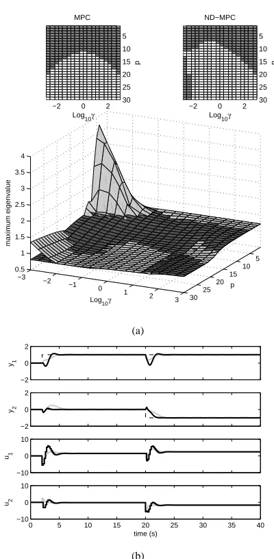
Fig. 1. Stability regions and maximum closed-loop

eigenvalues forα =0.1 (a) and control

perfor-mances withγ=0.01 and p=20 (b).

The corresponding discrete-time state-space realiza-tion is decomposed in two SISO subsystems.

Assum-ing that input u1controls output y1and input u2

con-trols output y2, the coefficientα represents a measure

of the interactions.

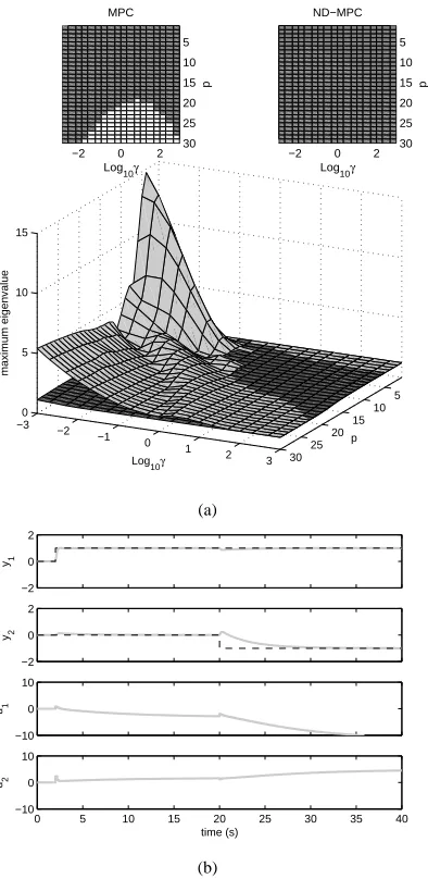
The maximum eigenvalues computed by the dynamic matrices obtained with the previous stated theorems are plotted in the three dimensional graphs of Figures 1(a), 2(a) and 3(a). The Z axis of these plots represents the maximum eigenvalue for the centralized MPC (dark gray surface) and the decentralized MPC with communication (light gray surface). The X and Y

axis represent the logarithm of the weightγ and the

prediction horizon p, respectively. The corresponding stable region (white surface) is represented in the upside part of these plots both for the centralized and the decentralized case. For each plant, the control performances of ND-MPC (black lines) are compared with the centralized MPC (gray lines) for a given combination of the parameters, as shown in Figures 1(b), 2(b) and 3(b).

−2 0 2 5 10 15 20 25 30

p

Log

10γ

MPC

−2 0 2 5 10 15 20 25 30

p

Log

10γ

ND−MPC

5 10 15 20 25 30

−3 ₋₂

−1 ₀

1

2 ₃

0.5 1 1.5 2 2.5 3 3.5 4

p

Log

10γ

maximum eigenvalue

(a)

−2 0 2

y1

−2 0 2

y2

−10 0 10

u1

0 5 10 15 20 25 30 35 40

−10 0 10

u2

time (s)

(b)

Fig. 2. Stability regions and maximum closed-loop

eigenvalues forα =0.5 (a) and control

perfor-mances withγ=0.01 and p=20 (b).

In the proposed examples, which are a set within the performed numerical tests, the stability performances

depend on the choice of the tuning parametersγ and

p. In particular the stability of the closed-loop system

is guaranteed for different combinations of the tun-ing parameters. A wider range of tuntun-ing parameters is available for weak interactions whereas a smaller stability region characterizes plants with strong actions. At the same time, more weak are the inter-actions, more ND-MPC shows control performances similar to centralized MPC. Often, when MPC is sta-ble, ND-MPC has the same maximum eigenvalues; in some cases ND-MPC seems to be even better.

−2 0 2 5 10 15 20 25 30

p

Log

10γ

MPC

−2 0 2 5 10 15 20 25 30

p

Log

10γ

ND−MPC

5 10 15 20 25 30

−3 ₋₂

−1 ₀

1

2 ₃

0 5 10 15

p

Log

10γ

maximum eigenvalue

(a)

−2 0 2

y1

−2 0 2

y2

−10 0 10

u1

0 5 10 15 20 25 30 35 40

−10 0 10

u2

time (s)

(b)

Fig. 3. Stability regions and maximum closed-loop

eigenvalues for α =2 (a) and control

perfor-mances withγ=0.01 and p=30 (b).

6. CONCLUSIONS AND FUTURE WORKS

In this paper a stability analysis tool for tuning ND-MPC architectures has been presented. The provided examples show that the proposed ND-MPC can often stabilize the process with a proper choice of the tuning parameters. In these regions the maximum eigenvalues approach that ones of the centralized case. However, in some cases, ND-MPC is not able to stabilize the process and other strategies must be considered.

In this work the unconstrained MPC for linear pro-cess with acpro-cessible state has been considered. Fu-ture works are needed for extending these conclu-sions in the more general case of constrained MPC. Techniques for obtaining explicit solutions in the con-strained case have already been investigated in litera-ture (Tøndel et al., 2003). Therefore, these techniques can potentially be used for extending the proposed approach to the constrained ND-MPC. Furthermore also robustness results (Bemporad and Morari, 1999) with respect to model uncertainties and disturbances

are needed. For instance, a study about the effect that perturbations on the model matrices produce on the closed-loop eigenvalues can be performed.

7. REFERENCES

Bemporad, A. and M. Morari (1999). Robust model predictive control: A survey. In: Robustness in

Identification and Control, Lecture Notes in Con-trol and Information Sciences (A. Garulli, A. Tesi

and A. Vicino, Eds.). Vol. 245. pp. 207–226. Springer. London.

Camponogara, E. (2000). Controlling networks with collaborative nets. PhD thesis. Carnegie Mellon. Camponogara, E., D. Jia, B. H. Krogh and S.

Taluk-dar (2002). Distributed model predictive control.

IEEE Control Syst. Mag. 22, 44–52.

Cheng, X. and B. H. Krogh (2001). Stability-constrained model predictive control. IEEE

Trans. on Aut. Cont. 46, 1816–1820.

El-Farra, N. H., A.Gani and P. D. Christofides (2004). Fault-tolerant control of multi-unit process sys-tems using communication networks. In: 7th

IFAC Symposium on Dynamics and Control of Proc. Syst.. Prague, CZ.

Gudi, Ravindra D., James B. Rawlings, Aswin Venkat and N. Jabbar (2004). Identification for decen-tralized mpc. In: DYCOPS. Boston, MA. Jia, D. (2003). Distributed coordination in multiagent

control systems through model predictive con-trol. PhD thesis. Carnegie Mellon.

Jia, D. and B. H. Krogh (2001). Distributed model predictive control. In: Proceedings of the A.C.C.. Vol. 4. pp. 2767–2772.

Katebi, M. R. and M. A. Johnson (1997). Predictive control design for large-scale systems..

Automat-ica 33, 421–425.

Longhi, S., R. Trillini and M. Vaccarini (2005). Appli-cation of a networked decentralized MPC to syn-gas process in oil industry. In: 16th IFAC World

Congress. Prague, CZ.

Motee, Nader and Bijan Sayyar-Rodsari (2003). Op-timal partitioning in distributed model predictive control. In: Proceedings of the American Control

Conference. Denver, Colorado. pp. 1866–1870.

Tøndel, P., T. A. Johansen and A. Bemporad (2003). An algorithm for multi-parametric quadratic pro-gramming and explicit mpc solutions.

Automat-ica 39(3), 489–497.

Vaccarini, M., S. Longhi and M.R. Katebi (2006). State space stability analysis of unconstrained decentralized model predictive control systems. In: Proceedings of the American Control

Confer-ence. Minneapolis, Minnesota. To be published.

Venkat, A. N., J. B. Rawlings and S. J. Wright (2005). Stability and optimality of distributed model pre-dictive control. CDC-ECC Joint Conference. ˇSiljak, D. D. (1996). Decentralized control and

com-putations: status and prospects. Annual Reviews