Int. J. Electrochem. Sci., 10 (2015) 6044 - 6056
International Journal of
ELECTROCHEMICAL
SCIENCE
www.electrochemsci.orgPrediction of Zeta Potential of Decomposed Peat via Machine
Learning: Comparative Study of Support Vector Machine and
Artificial Neural Networks
Hao Li1,2,#, Fudi Chen1,#, Kewei Cheng3, Zheze Zhao4 and Dazuo Yang1,5,* 1
Key Laboratory of Marine Bio-Resources Restoration and Habitat Reparation in Liaoning Province, Dalian Ocean University, Dalian, Liaoning, China
2
College of Chemistry, Sichuan University, Chengdu, Sichuan, China 3
School of Computing, Informatics, and Decision Systems Engineering (CIDSE), Ira A. Fulton Schools of Engineering, Arizona State University, Tempe, Arizona, USA
4
College of Agriculture, Health and Natural Resources, University of Connecticut, Farmington, Connecticut, USA
5
College of Life Science and Technology, Dalian University of Technology, Dalian, Liaoning, China # These authors contributed equally to this work.
*
E-mail: [email protected]
Received: 5 May 2015 / Accepted: 9 June 2015 / Published: 24 June 2015
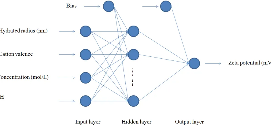
Zeta potential is crucial for practical applications in electrochemistry. However, the precise deterimination of zeta potential of decomposed peat is complex and has high requirements to related instructments. Previous study shows that zeta potential of decomposed peat can be predicted by back-propagation (BP) neural network. However, it lacks available comparisons and neglects the importance of the decomposed stages of peat and the required training times. Here, to extend this research, we propose a series of novel machine learning techniques including support vector machine (SVM) and artificial neural networks (ANNs) to predict the zeta potential of decomposed peat. Four indicators including hydrated radius (nm), cation valence, concentration (mol/L) and pH are set as independent variables while zeta potential (mV) is set as the dependent variable. The SVM, general regression neural network (GRNN) and multilayer feed-forward neural networks (MLFNs) are developed in different decomposed stages, including the slightly decomposed peat, the highly decomposed peat and all decomposed peat. Results show that separating the models based on the decomposed stages have better prediction results than taking all decomposed peat in one model. During our studies, the SVM is the best model for the prediction to the slightly decomposed peat (RMS error: 2.37, training time: 1s), while the GRNN is the best model for the prediction to the highly decomposed peat (RMS error: 2.20, training time: 1s).
1. INTRODUCTION
In the field of electrochemistry, zeta potential, the electric potential in the interfacial double layer at the location of the slipping plane, is the potential difference between the stationary layer of fluid attached to the dispersed particle and the dispersion medium [1-3]. Studies show that zeta potential is mainly caused by the net electrical charge contained in the region bounded by the slipping plane and influenced by the location of it [4-8]. With the development of electrochemical technology, there are currently several determination methods for zeta potentials, including electro-osmosis, electrophoresis, streaming potentiometry and ultrasonic method [1].
Zeta potential is a crucial indicator of the stability of colloidal dispersions [9-14]. For the decomposed peat, zeta potential also plays a crucial role in related studies. However, in practical applications, the exact determination of zeta potential of decomposed peat is complex and requires a series of operations and necessary electrochemical instruments, which wastes too much time and manpower. To reduce experimental works, previous studies used back-propagation (BP) neural network to predict the zeta potential of decomposed peat in the presence of different cations [15]. However, this study only discussed one possible model for the prediction, which neglected necessary comparisons with different artificial neural networks (ANNs) and other powerful machine learning techniques. Also, the decomposed stages and the effects of number of neurons to the required training time were also neglected. Therefore, to improve the prediction technique, it is necessary for us to find out a better model that takes all these neglected items into consideration, including i) prediction effects of different models; ii) errors of testing and required training times of the models and iii) numbers of neurons (numbers of nodes) in the hidden layers of ANNs. Here, to find out a better model for the prediction of zeta potential of decomposed peat, we use novel machine learning techniques including novel ANNs and support vector machine (SVM) to develop a series of prediction models for decomposed peat in the presence of different cations. Two stages of decomposed peats defined by the classification method [15] including the slightly and the highly decomposed peats are taken into different considerations. Selections of results are based on the comprehensive performances of different models, including the change regulation of results of ANNs with different nodes. Comparisons are made among different models according to the testing results, which contain the root mean square error (RMS error), training time and prediction accuracy.
2. MATERIALS AND METHODS
2.1 Introduction to Experiments
Statistical experimental results of the determination of zeta potential of decomposed peat are shown in Table 1.
Table 1. Statistical experimental results of the determination of zeta potential of decomposed peat (data extracted from Asadi's research [15] ).
Statistical item Hydrated radius (nm)
Cation valence Concentration (mol/L)
pH Zeta potential (mV)
Minimum 0.33 1 0.0001 2.790 -32.37
Maximum 0.48 3 0.0010 11.77 -1.500
Average 0.39 N/A 0.0034 7.260 -15.69
2.2 Support Vector Machine (SVM)
[image:3.596.45.552.164.225.2]SVM is a powerful machine learning technique mainly on the basis of statistical learning theory [16]. Based on the limited information of samples between the complexity and learning ability of models, this theory has an outstanding ability of global optimization for improving generalization. In terms of linear separable binary classification, finding the optimal hyperplane, a plane that separates all samples with the maximum margin, is the main principle of SVM [17, 18]. The plane not only helps improve the predictive ability of the model, but also helps reduce the error which occurs occasionally when classifying. Figure 1 [19] shows the optimal hyperplane, with “+” representing the samples of type 1 and “−” representing the samples of type −1.
[image:3.596.121.502.432.722.2]
Figure 2 illustrates the main structure of a typical SVM [19]. The letter “K” represents kernels [20]. As it can be seen from Figure 2, it is a small subset extracted from the training data by relevant algorithm that consists of the SVM. For applications, choosing suitable kernels and appropriate parameters is of great importance to get a good prediction accuracy. Nevertheless, there is still no existing international standard for users to choose these parameters. Under most circumstances, the comparison of experimental results, the experiences from copious calculating, and the use of cross validation that is available in software package are able to help us solve this problem in a relatively reliable way [19,21,22].
Figure 2. Main structure of a support vector machine [19].
2.3 Artificial Neural Networks (ANNs)
Figure 3. Schematic structure of an ANN for the prediction of zeta potential.
3. RESULTS AND DISCUSSION
3.1 Model Development
Here, we use novel machine learning techniques to analyze the experimental results provided by previous research [15]. 80% data group was set as the training set, while 20% data group was set as the testing set. The SVM was developed by the Matlab software. The ANNs were constructed by the NeuralTools® software (trial version, Palisade Corporation, NY, USA). General regression neural network (GRNN) [26-28] and multilayer feed-forward neural network (MLFN) [29-31] were chosen as the algorithms of ANNs.
[image:5.596.130.469.648.767.2]The RMS error, required training time and prediction accuracy (under the tolerance of 30%) were used as indicators to measure the performances of the SVM and ANNs. The number of nodes of MLFNs were set from 2 to 25, from which we could find out the change regulation of the MLFNs when dealing with the development processes. Three groups of models were developed respectively, including the slightly decomposed peat (Table 2), the highly decomposed peat (Table 3) and all decomposed peat (which contains both slightly and highly decomposed peats, Table 4).
Table 2. Machine learning models for the prediction of zeta potential of the slightly decomposed peat.
Model RMS Error
Training Time
Prediction Accuracy
SVM 2.37 0:00:01 100%
GRNN 3.23 0:00:01 84.6%
MLFN: 2 Nodes 2.64 0:00:39 92.3%
MLFN: 3 Nodes 2.40 0:00:44 100%
MLFN: 4 Nodes 3.14 0:00:46 84.6%
MLFN: 6 Nodes 3.09 0:01:04 84.6%
MLFN: 7 Nodes 2.83 0:01:09 92.3%
MLFN: 8 Nodes 3.43 0:01:22 84.6%
MLFN: 9 Nodes 5.16 0:01:39 69.2%
MLFN: 10 Nodes 4.61 0:01:55 76.9%
MLFN:11 Nodes 6.29 0:01:51 69.2%
MLFN: 12 Nodes 5.96 0:02:04 69.2%
MLFN:13 Nodes 5.81 0:02:27 69.2%
MLFN: 14 Nodes 2.93 0:02:40 84.6%
MLFN: 15 Nodes 3.45 0:03:03 84.6%
MLFN: 16 Nodes 8.72 0:03:26 61.5%
MLFN: 17 Nodes 5.03 0:03:35 76.9%
MLFN: 18 Nodes 4.33 0:03:34 76.9%
MLFN: 19 Nodes 3.15 0:03:56 84.6%
MLFN: 20 Nodes 6.33 0:04:09 69.2%
MLFN: 21 Nodes 4.21 0:04:54 76.9%
MLFN: 22 Nodes 3.54 0:05:19 84.6%
MLFN: 23 Nodes 4.43 0:05:34 76.9%
MLFN: 24 Nodes 3.95 0:06:10 76.9%
[image:6.596.130.468.71.370.2]MLFN: 25 Nodes 3.25 0:06:30 84.6%
Table 2 shows that the SVM and MLFN with 3 nodes have the lowest RMS errors (2.37 and 2.40 respectively) and the highest prediction accuracies (both 100%). The SVM and GRNN have the shortest training times (both 1s). In sum, the SVM is the most suitable model for the prediction of zeta potential of the slightly decomposed peat because of its low RMS error, high prediction accuracy and short required training time.
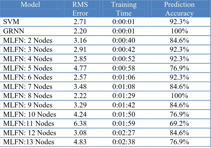
Table 3. Machine learning models for the prediction of zeta potential of the highly decomposed peat.
Model RMS Error
Training Time
Prediction Accuracy
SVM 2.71 0:00:01 92.3%
GRNN 2.20 0:00:01 100%
MLFN: 2 Nodes 3.16 0:00:40 84.6%
MLFN: 3 Nodes 2.91 0:00:42 92.3%
MLFN: 4 Nodes 2.85 0:00:52 92.3%
MLFN: 5 Nodes 4.77 0:00:58 76.9%
MLFN: 6 Nodes 2.57 0:01:06 92.3%
MLFN: 7 Nodes 3.48 0:01:08 84.6%
MLFN: 8 Nodes 2.22 0:01:29 100%
MLFN: 9 Nodes 3.29 0:01:42 84.6%
MLFN: 10 Nodes 4.24 0:01:50 76.9%
MLFN:11 Nodes 6.38 0:01:59 69.2%
MLFN: 12 Nodes 3.08 0:02:27 84.6%
[image:6.596.129.468.536.773.2]
MLFN: 14 Nodes 4.65 0:02:47 76.9%
MLFN: 15 Nodes 3.92 0:03:01 84.6%
MLFN: 16 Nodes 4.90 0:03:13 76.9%
MLFN: 17 Nodes 4.75 0:03:54 76.9%
MLFN: 18 Nodes 5.53 0:04:10 69.2%
MLFN: 19 Nodes 6.25 0:05:08 69.2%
MLFN: 20 Nodes 4.71 0:05:42 76.9%
MLFN: 21 Nodes 3.77 0:05:23 84.6%
MLFN: 22 Nodes 3.39 0:06:38 84.6%
MLFN: 23 Nodes 3.73 0:06:33 84.6%
MLFN: 24 Nodes 5.23 0:07:26 69.2%
MLFN: 25 Nodes 10.19 0:09:24 0.00%
[image:7.596.131.469.402.759.2]Table 3 shows that the GRNN and MLFN with 8 nodes have the lowest RMS errors (2.20 and 2.22 respectively) and the highest prediction accuracies (both 100%). However, the MLFN with 8 nodes required a much longer training time than that of the GRNN. Therefore, the GRNN is considered as the most suitable model for the prediction of zeta potential of the highly decomposed peat.
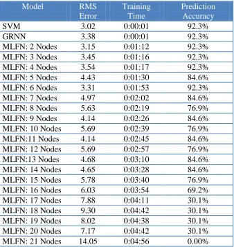
Table 4. Machine learning models for the prediction of zeta potential of all (both slightly and highly) decomposed peats.
Model RMS Error
Training Time
Prediction Accuracy
SVM 3.02 0:00:01 92.3%
GRNN 3.38 0:00:01 92.3%
MLFN: 2 Nodes 3.15 0:01:12 92.3%
MLFN: 3 Nodes 3.45 0:01:16 92.3%
MLFN: 4 Nodes 3.54 0:01:17 92.3%
MLFN: 5 Nodes 4.43 0:01:30 84.6%
MLFN: 6 Nodes 3.31 0:01:53 92.3%
MLFN: 7 Nodes 4.97 0:02:02 84.6%
MLFN: 8 Nodes 5.63 0:02:19 76.9%
MLFN: 9 Nodes 4.14 0:02:26 84.6%
MLFN: 10 Nodes 5.69 0:02:39 76.9%
MLFN:11 Nodes 4.14 0:02:45 84.6%
MLFN: 12 Nodes 5.69 0:02:57 76.9%
MLFN:13 Nodes 4.68 0:03:10 84.6%
MLFN: 14 Nodes 4.65 0:03:28 84.6%
MLFN: 15 Nodes 5.78 0:03:40 76.9%
MLFN: 16 Nodes 6.03 0:03:54 69.2%
MLFN: 17 Nodes 7.88 0:04:11 30.1%
MLFN: 18 Nodes 9.30 0:04:42 30.1%
MLFN: 19 Nodes 8.02 0:04:38 30.1%
MLFN: 20 Nodes 7.17 0:04:42 30.1%
MLFN: 22 Nodes 14.54 0:06:12 0.00%
MLFN: 23 Nodes 10.94 0:06:23 0.00%
MLFN: 24 Nodes 15.70 0:06:03 0.00%
[image:8.596.128.471.70.130.2]MLFN: 25 Nodes 20.99 0:05:41 0.00%
Table 4 shows that the SVM has the lowest RMS error (3.02) and the shortest required training time (1s). However, it can be apparently seen that results presented in Tables 2 and 3 are generally better than those in Table 4, with generally lower RMS errors and higher prediction accuracies. This phenomenon indicates that the best prediction results may appear when prediction models for the slightly and the highly decomposed peats are developed respectively. If the two stages of decomposed peats are used for making a united model (like the models presented in Table 4), the learning process may be confused because the zeta potentials of the two stages of decomposed peats may have different relationships with the independent variables we chose.
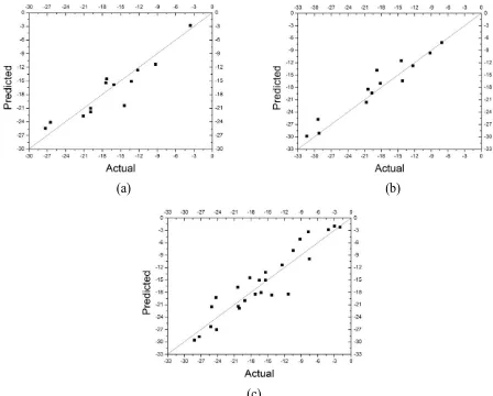
(a) (b)
(c)
[image:8.596.67.515.309.669.2]
(b)] are relatively closer to their actual values than those of the SVM for all decomposed peat [Figure 4 (c)]. Therefore, the SVM is shown as the best model for the prediction of zeta potential for the slightly decomposed peat, while the GRNN is shown as the best model for that of the highly decomposed peat.
3.2 Robustness Analysis for ANNs
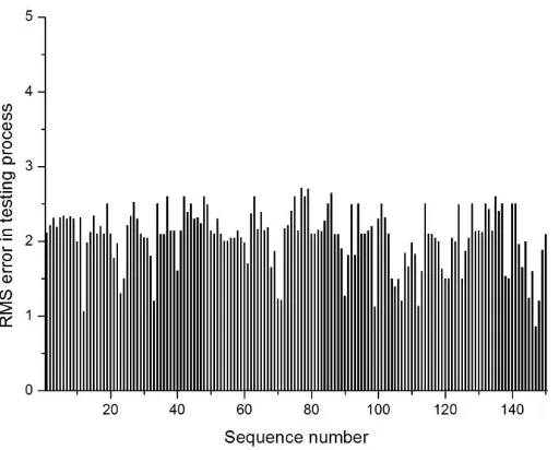
According to the principles of the SVM, it has an excellent robustness, which means that it has a good reproducibility. However, the randomness in the initial process is one of the characteristics of ANNs, which leads to different results in repeated experiments. Now that the results presented in this article has shown that the GRNN is the best for the highly decomposed peat, the reproducibility of the GRNN still cannot be neglected. To test the robustness of the GRNN in predicting the zeta potential of the highly decomposed peat, 150 repeated experiments were done (Figure 5). They show that although there exists fluctuations, the changes of RMS errors are stable, indicating that the GRNN is robust in predicting the zeta potential of the highly decomposed peat using the provided data. Therefore, the GRNN is proved to be available in practical applications.
Figure 5. Repeated experimental results of the GRNN in predicting the zeta potential of the highly decomposed peat.
[image:9.596.169.425.342.548.2]
(a)
(b)
(c)
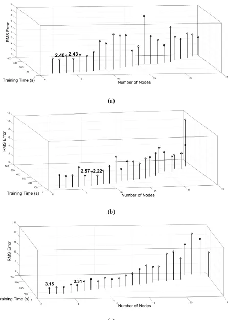
[image:10.596.80.526.81.707.2]
Figure 6 shows that in all the three prediction duties, RMS errors of the MLFNs are comparatively stable in low nodes and the required training times generally increase with the increase of the number of nodes. Meanwhile, the RMS errors in high number of nodes are not stable enough. Therefore, if we have to use an MLFN as an alternative, the MLFNs with low number of nodes can be considered.
3.3 Comparisons with Previous Studies
To make comprehensive comparisons between our models and previous approaches, the discussion should be divided into two parts. The first part is the comparisons between machine learning techniques and the conventional measurements for zeta potentials. The second part is the comparisons among different machine learning techniques for zeta potentials.
So far, there are various conventional approaches for measuring zeta potentials. In many different cases, some of these approaches have been widely-used in relevant fields, including the use of Smoluchowski equation [32], the use of the relationship between measured electrical signals and zeta potentials [33,34], the use of effects of ions to the zeta potentials [35] and electrophoresis technique [36]. However, all these approaches require a large number of experimental and calculation works, which have high requirements to experimental instruments and meanwhile, waste too much time and manpower. In contrast, based on the "learned" experimental data, machine learning techniques have comparatively better performances to predict the zeta potential in our cases due to its powerful capacity of finding out the relationship between independent and dependent variables. When the training process of a model is completed, users can only input the values of independent variables obtained by simple determination processes, and then the precise predicted results can be outputted automatically and quickly. Here, we use the decomposed peat as a typical example, showing that machine learning techniques have strong potentials for practical applications to measure zeta potentials. Also, with the development of computer science, machine learning models now can be developed using user-friendly softwares or packages [19,21,22,37,38]. Based on the reasons above, machine learning, our novel techniques for measuring zeta potentials, have significant advantages when being compared with other conventional popular approaches.
the required training times into consideration can help us obtain better machine learning models for the prediction of the zeta potential. In addition, the use of the SVM also shows that as a novel and strong machine learning tool, SVM has great potential applications in electrochemical field. Further related studies should not only discuss the availability of ANNs, but also introduce the results of SVM when predicting. Only by making comparisons among ANNs, SVM and other prediction models, can we define the most suitable models in related prediction studies.
4. CONCLUSION
Here, we successfully show that better machine learning prediction models of zeta potential of decomposed peat can be obtained by separating the decomposed peat into two stages, the slightly and the highly decomposed peats. Models are proposed respectively to find out the best prediction results for zeta potentials of the two stages. Results show that the SVM is the most suitable model for the prediction of zeta potential of the slightly decomposed peat while the GRNN is the most suitable model for the prediction of zeta potential of the highly decomposed peat due to their low RMS errors, high prediction accuracies and short training times.
ACKNOWLEDGEMENT
This work was funded by the National Marine Public Welfare Research Project (nos. 201305002 and 201305043), National Natural Science Foundation of China (no. 30901107), and the Project of Marine Ecological Restoration Technology Research to the Penglai 19-3 Oil Spill Accident (no. 19-3YJ09).
References
1. R. J. Hunter, Zeta potential in colloid science: principles and applications, Academic press (2013). 2. B. J. Kirby and E. F. Hasselbrink, Electrophoresis, 25 (2004) 187.
3. C. Schwer and E. Kenndler, Anal. Chem., 63 (1991) 1801. 4. J. A. Schellman and D. Stigter, Biopolymers, 16 (1977) 1415.
5. C. Schwer and E. Kenndler, Anal. Chem., 63 (1991) 1801.
6. R. Van Hal, J. Eijkel and P. Bergveld, Adv. Colloid. Interfac., 69 (1996) 31. 7. A. Revil, P. Pezard and P. Glover, J. Geophys. Res., 104 (1999) 20021. 8. P. Sennett, J. P. Olivier, Ind. Eng. Chem., 57 (1965) 32.
9. B. Heurtault, P. Saulnier, B. Pech, J. E. Proust and J. P. Benoit, Biomaterials, 24 (2003) 4283. 10. A. Morfesis, A. M. Jacobson, R. Frollini, M. Helgeson, J. Billica and K. R. Gertig, Ind. Eng. Chem.
Res.,48 (2008) 2305.
11. S. W. Lee, S. D. Park, S. Kang, I. C. Bang and J. H. Kim, Int. J. Heat. Mass Tran., 54 (2011) 433. 12. H. Moayedi, A. Asadi, F. Moayedi and B. B. Huat, Int. J. Electrochem. Sci., 6 (2011) 1294. 13. J. A. Brant, H. Lecoanet and M. R. Wiesner, J. Nanopart. Res., 7 (2005) 545.
14. E. F. de la Cruz, Y. Zheng, E. Torres, W. Li, W. Song and K. Burugapalli, Int. J. Electrochem. Sci., 7 (2012) 3577.
15. A. Asadi, H. Moayedi, B. B. Huat, F. Z. Boroujeni, A. Parsaie and S. Sojoudi, Int. J. Electrochem. Sci., 6 (2011) 1146.
16. N. Deng, Y. Tian and C. Zhang, Support vector machines: optimization based theory, algorithms, and extensions, CRC Press (2012)
18. Y. Shen, Z. He, Q. Wang and Y. Wang, IEEE Instrumentation and Measurement Technology Conference Proceedings 2012, (2012) 1977.
19. H. Li, W. Leng, Y. Zhou, F. Chen, Z. Xiu and D. Yang, The Scientific World Journal, 2014 (2014). 20. D. W. Kim, K. Lee, D. Lee and K. H. Lee, Pattern Recogn. Lett., 26 (2005) 879.
21. R. E. Fan, K. W. Chang, C. J. Hsieh, X. R. Wang and C. J. Lin. Mach. Learn. Res., 9 (2008) 1871. 22. Q. Guo, Y. Liu. Ecography, 33 (2010) 637.
23. J. J. Hopfield, IEEE Circuit Devic., 4 (1988) 3.
24. B. Yegnanarayana, Artificial neural networks, PHI Learning Pvt. Ltd. (2009). 25. J. E. Dayhoff. and J. M. DeLeo, Cancer, 91 (2001) 1615.
26. D. F. Specht, Neural Networks, IEEE Transactions on, 2 (1991) 568. 27. D. Tomandl and A. Schober; IEEE T. Neur. Net. Lear., 14 (2001) 1023. 28. D. F. Specht, IEEE T. Neur. Net. Lear., 6 (1993) 1033.
29. D. Svozil, K. Vladimir and P. Jiri, Chemometr. Intell. Lab., 39 (1997) 43.
30. J. Smits, W. Melssen, L. Buydens and G. Kateman. Chemometr. Intell. Lab., 22 (1994) 165. 31. J. Ilonen, J.-K. Kamarainen and J. Lampinen, Neural Process. Lett., 17 (2003) 93.
32. A. Sze, D. Erickson, L. Ren and D. Li, J. Colloid Interf. Sci., 261 (2003) 402.
33. Y. Song, K. Zhao, J. Wang, X. Wu, X. Pan, Y. Sun and D. Li, J. Colloid Interf. Sci., 416 (2014) 101.
34. Y. Song, K. Zhao, M. Li, X. Wu, X. Pan and D. Li, Anal. Chim. Acta, 863 (2015) 689. 35. P. Moulin and H. Roques, J. Colloid Interf. Sci., 261 (2003) 115.
36. C. Yang, T. Dabros, D. Li, J. Czarnecki and J. Masliyah, J. Colloid Interf. Sci., 243 (2001) 128. 37. C-C. Chang and C-J. Lin, ACM T. Intel. Syst. Tec., 2 (2011).
![Table 1. Statistical experimental results of the determination of zeta potential of decomposed peat (data extracted from Asadi's research [15] )](https://thumb-us.123doks.com/thumbv2/123dok_us/1888838.146412/3.596.45.552.164.225/statistical-experimental-results-determination-potential-decomposed-extracted-research.webp)
![Figure 2 illustrates the main structure of a typical SVM [19]. The letter “K[20]. As it can be seen from Figure 2, it is a small subset extracted from the training data by relevant algorithm that consists of the SVM](https://thumb-us.123doks.com/thumbv2/123dok_us/1888838.146412/4.596.178.453.227.395/figure-illustrates-structure-extracted-training-relevant-algorithm-consists.webp)