Development of a 2D boundary element method to model Schroeder acoustic diffusers

(1)

Development of a 2D

Boundary Element Method

to model Schroeder Acoustic Di

↵

users

Andrew Lock 098911

October 2014

Supervisor: Dr Damien Holloway

(2)

This Thesis to the best of my knowledge and belief contains no material published or unpublished that was written by another person, nor any material that infringes copy-right, nor any material that has been accepted for a degree or diploma by University of Tasmania or any other institution, except by way of background information and where due acknowledgement is made in the text of the thesis.

This Thesis is the result of my own investigation, except where otherwise stated.

Other sources are acknowledged in the text giving explicit references. A list of

ref-erences is appended.

Signed:

Date:

I hereby give consent for my Thesis to be available for photocopying, inter-library loan, electronic access to UTAS sta↵ and students via the UTAS Library, and for the title and summary to be made available to outside organisations.

Signed:

(3)

Abstract

(4)

Acknowledgements

Firstly, I would like to express my sincere thanks to Dr Damien Holloway, not only for his knowledge, enthusiasm, and generous time on this project, but also for his wider contribution to our undergraduate studies.

To my parents, Sally and Chris. Thank you for your constant support through-out my education, in particular during this final year.

(5)

List of Figures

2.1.1 Illustration of pressure waves at a snapshot in time (Everest & Pohlmann,

2009) [11] . . . 5

2.1.2 Superposition of multiple sine waves. . . 6

2.3.1 Sound wave reflection . . . 8

2.3.2 Incident wave spatially di↵used . . . 9

2.3.3 Cylindrical wave reflected from a Schroeder di↵user calculated using an FDTD model. . . 9

2.3.4 Comparison ofcd,cp and cn for an N = 23 QRD. . . 11

2.4.1 Example of energy lobe di↵raction pattern fromN = 7 QRD at 4 times f0. 15 2.4.2 Cross section of N=7 MLS di↵user. . . 16

2.4.3 Example ofN = 7 QRD in single and repeating periods. . . 17

2.4.4 An N = 7 QRD array of multiple repeating periods. . . 19

2.4.5 An N = 7 QRD design with two levels of fractals nested within each well. 21 2.4.6 QRD and di↵usion pattern for one-dimensional and two-dimensional QRDs. 22 2.5.1 A two-dimensional di↵user modelled using a three-dimensional BEM. . . . 25

3.2.1 Flowchart of current BEM code. . . 29

4.7.1 Absolute value of Hankel functions of constant kand increasingr. . . 36

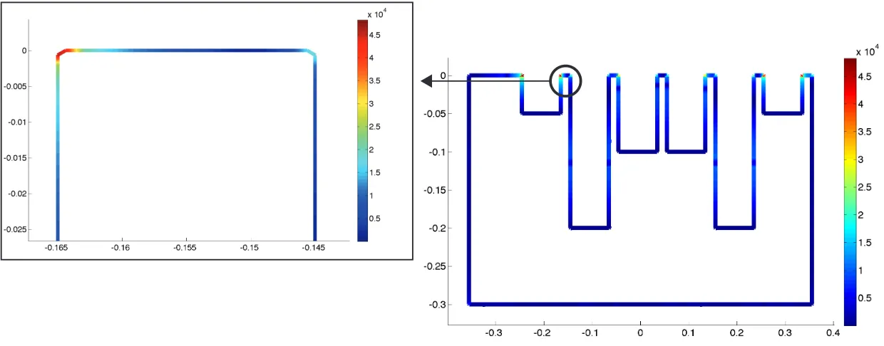
5.1.1 Surface pressures of an infinite square column in a point source acoustic field. . . 44

5.1.2 QRD surface pressure gradient magnitude . . . 45

5.1.3 Infinite square column discretisation with and without edge refinement. . 46

5.1.4 QRD model with hollow cavity to check for non-unique solutions. . . 47

5.2.1 Diagram of di↵usion model from an infinite cylinder. . . 49

5.2.2 Di↵usion from a cylinder due to a plane wave. . . 49

5.2.3 Comparison of di↵usion lobe positions (dB) for anN = 7 QRD. . . 51

(10)

5.2.5 Convergence of di↵usion coefficient at 2500 Hz for QRD as modelled in

Figure 5.2.4 . . . 52

5.2.6 Timing comparison between original and optimised code. . . 54

5.2.7 Comparison of solution time and convergence from 3 BEM code versions. 54

5.2.8 Example of convergence testing with varying panel width with forN = 7

QRD. . . 57

5.2.9 Maximum element size for which convergence errors are not dominated

by thin panel errors. . . 58

5.2.10Convergence study with normalised element lengthen. . . 60

7.1.1 Performance of QRD arrays of variableN in a plane wave incident field. . 68

7.1.2 Comparison of QRD performance in di↵erent acoustic fields. . . 69

7.1.3 Performance data for N = 7 QRD arrays with varying P. . . 70

7.1.4 Comparison of regular and phase shifted QRD performance. . . 71

7.2.1 Four fractal-type QRD designs tested for di↵usion frequency bandwidth. . 73

7.2.2 Comparison of three fractal designs and regular QRD performance. . . 73

7.3.1 E↵ect of thin panel width on di↵user performance . . . 75

A.1.1QRD di↵usion data. . . 86

A.2.1Comparison of di↵erent acoustic fields for QRDs of comparable wT and

(11)

List of Tables

2.4.1 Quadratic Residue Sequence calculation example for N = 7 . . . 16

2.4.2 Primitive root Sequence calculation example forN = 7,r = 3 . . . 20

2.4.3 Example of a regular and phase shifted Quadratic Residue Sequence . . . 21

3.2.1 BEM code subroutines . . . 28

5.1.1r threshold values and Gaussian Quadrature points. . . 42

5.2.1 Comparison of receiver pressure error when compared to an analytic solution 50 5.2.2 Solution time improvements breakdown . . . 55

5.2.3 QRD details for convergence testing, as shown in Figure 5.2.10 . . . 59

B.1.1BEM program steps . . . 89

B.3.1Table of QRD dimensions for test as shown in Figure 7.1.1 . . . 93

B.4.1Specifications of computer used in code timing . . . 93

(12)

Nomenclature

f Frequency (Hz)

f0 Design frequency (Hz)

fc Critical frequency (Hz)

Wavelength (m)

c Critical wavelength (m)

k Wavenumber (m 1₎

Acoustic potential p Pressure (Pa)

BEM Boundary Element Method QRD Quadratic Residue Di↵user PRD Primitive Root Di↵user

N Prime number used in QRD and PRD sequence r Primitive root of N

dmax Maximum well depth of QRD (m)

w Width of QRD well (m)

w_P Width of well dividing panel (m)

w_T Width of combined well and panel divider (m) N w_T Period width (m)

P Number of periods of sequential di↵user in array cd, Di↵usion coefficient for incident angle

cr, Reference di↵usion coefficient for incident angle

cn, Normalised di↵usion coefficient for incident angle

s Scattering coefficient

↵ Absorption coefficient

Angle of sound wave from normal to di↵user r Distance between two elements (m)

ka Dimensionless radius of cylindrical di↵user kr Dimensionless radius of o↵-surface receivers e Element size (m)

emax Maximum element size (m)

(13)

Part I

(14)

Chapter 1 Introduction

An acoustic di↵user is an object or surface profile designed to provide a di↵use reflection

from an incident sound wave. While nearly all reflective surfaces will o↵er some degree

of di↵usion, an acoustic di↵user is designed to produce high levels of di↵usion or specific

di↵usion characteristics, often for a design application or frequency range. Di↵usion can

be either temporal (time-related) or spatial, and is a useful tool in the in acoustic

treat-ment of spaces such as critical listening rooms and performance spaces, often to create

a more even sound field or to avoid strong reflections [7]. Where traditionally acoustic

absorbers have been used to avoid undesirable acoustic e↵ects, there is a growing trend

towards the use of di↵users instead [7], and this has increased the need to accurately

model their performance.

The di↵usion produced by an object in an incident acoustic field can be described by

the sound pressure levels at points around the object, either as done experimentally by

Wiener [31] (1947) or through theoretical analysis. Methods of analysis include

analyt-ical solutions for some simple common geometries such as that of a cylinder published

by Morse [21] (1986), Finite Element Analysis, Finite-Di↵erence Time Domain (FDTD)

method, and the Boundary Element Method (BEM). Theoretical predictions are used in

the design and optimisation of acoustic di↵users, as well as predicting the performance

of existing di↵user shapes and surfaces.

Two final year engineering students, Nicholas Smith [28] (2013) and Luca Rocchi [23]

(2013), developed a MATLAB1 _{implementation of the BEM to model the performance}

of acoustic di↵users. Their findings aligned with Cox & D’Antonio [7], showing that for

many applications, the BEM is a superior method for di↵user analysis when compared

to other methods, in particular, Finite Element Analysis.

(15)

1.1 Objective and scope

The initial aim of this work is to further develop and document the BEM program

written by Rocchi and Smith. Accuracy and timing improvements to the BEM code are

achieved through.

• correction of errors in the original BEM code;

• analytical integration of diagonal matrix terms (see Chapter 4.8.2);

• variation in the number of Gaussian Quadrature integration points used in matrix

term calculations (see Chapter 4.8.1);

• code restructuring and in some cases complete replacement, to increase speed and

make use of MATLAB’s built-in acceleration features (see Chapter 5.1.2); and

• element size refinement in critical locations such as edges (see Chapter 5.1.4).

Increased functionality was also added, including:

• a formula derived from a detailed convergence study to determine the required

element size for a given frequency, geometry and level of accuracy;

• MATLAB functions written to automatically create QRD geometry with variable

dimensions and features (see Chapter 2.4.3.2);

• the capability to model a point source incident sound field in addition to a plane

wave field (see Chapter 4.3);

• frequency band modelling and averaging; and

• the calculation of the di↵usion coefficient, reference plate di↵usion coefficient and normalised di↵usion coefficient (see Chapter 2.3.3.1);

A detailed validation and convergence analysis was completed, and documentation

ac-companies this code to increase its usability. The second aim of this work is to use the

the developed code to predict the performance of Schroeder di↵users, with a focus on

(16)

1.2 Structure

This study is divided into three distinct parts. Part I introduces the topic, and discusses

related concepts and past research. Part II outlines the development of a MATLAB

BEM code used to model the scattering from objects within an acoustic field. Part III is

an investigation into the di↵usive properties of Schroeder di↵users using the BEM code.

A brief description of each chapter is included below.

Chapter 2: This chapter contains a review of current literature relevant to the topic,

including fundamental acoustic principles, the BEM, and common di↵user designs and

theory. Particular detail is paid to QRDs including recent developments in QRD design.

Chapter 3: An introduction is given to the MATLAB implementation of the BEM,

including descriptions of the code structure and instructions on executing the code.

Chapter 4: A detailed derivation of the BEM is presented, and the steps used to

solve a discretised form of the BEM are described.

Chapter 5: The development of the BEM code during this work is documented,

including the methods used to increase efficiency and accuracy. The code is thoroughly

tested, and the improvements are quantified. From a study of error and convergence, an

empirical equation is derived for the estimated accuracy when using the code to model

Schroeder di↵users.

Chapter 6: The scope of the investigation into Schroeder di↵users is outlined, and

the details used during di↵usion modelling are listed.

Chapter 7: Results from Schroeder di↵user BEM models are presented and

dis-cussed. The results are compared to the traditional design equations that describe the

performance of these di↵users.

Chapter 8: Conclusions and key findings are summarised, and further research is

(17)

Chapter 2 Literature Review

From published literature, this chapter will explain some of the fundamental

acous-tic principles including basic wave theory, absorption, reflection and di↵usion. Some

common di↵user shapes will then be discussed, with particular attention to Schroeder

di↵users. Recent developments in Schroeder di↵user design such as repeating periods,

modulated periods and fractals are discussed, along with state-of-the-art in BEM

acous-tic modelling.

2.1 Acoustic waves

An acoustic wave is the movement of pressure waves through an elastic medium, which

for most cases, and the focus of this work, is air. Figure 2.1.1 shows an illustration of

pressure waves at a snapshot in time, with the corresponding graphical representation.

The speed of soundc in air at normal temperature is c⇡343 m/s [11].

Figure 2.1.1: Illustration of pressure waves at a snapshot in time (Ever-est & Pohlmann, 2009) [11]

(18)

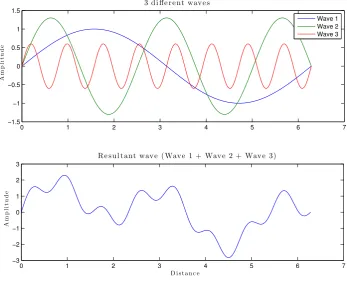
acoustic field is usually a superposition of pressure waves of di↵erent amplitudes and

frequencies, as shown in Figure 2.1.2. This concept also applies to the interaction

be-tween incident and di↵racted waves, and is the cause of comb filtering, as discussed in

Chapter 2.3.4.

0 1 2 3 4 5 6 7

−1.5

−1

−0.5 0 0.5 1 1.5

Am

p

li

tu

d

e

3 d iﬀe r e nt wav e s

0 1 2 3 4 5 6 7

−3

−2

−1 0 1 2 3

D i st an c e

Am

p

li

tu

d

e

Re su l t ant wav e ( Wav e 1 + Wav e 2 + Wav e 3)

[image:18.595.140.488.189.476.2]

Wave 1 Wave 2 Wave 3

Figure 2.1.2: Superposition of multiple sine waves.

2.2 Acoustic field types

The acoustic field in most environments consists of a mixture of incident sound from one

or more sources, and reflections from the ground, walls or objects within the acoustic

field. For the purposes of analysis during this investigation, the incident acoustic field is

simplified into two categories, a plane wave and point source, both of which ignore the

e↵ect of reflections.

2.2.1 Plane wave incident field

A plane wave incident field describes an acoustic field where, at any point in time,

(19)

is a reasonable approximation for a source at much larger distance from an object than

the object’s dimensions normal to the wave direction. On a two dimensional

applica-tion inx, y co-ordinates, a plane wave approaching from the positivey direction can be

assumed to have constant pressureP in the x direction at any point in time, @_@P_x = 0.

The rate at which pressure changes in the y direction is related to the amplitude and

frequency of the plane wave (see Chapter 4.3).

2.2.2 Point source incident field

For situations where the distance between an acoustic source is comparable to the

di-mensions of the object or receivers, the wavefront cannot be assumed to be planar.

A point source incident field represents an acoustic source originating from a singular

point within the sound field. For three dimensional applications, pressure waves radiate

spherically, whereas for two dimension applications, waves radiate cylindrically from the

source location. At any point in time, the pressure at a point is relative to the distance

from the source only, or @_@✓P = 0 where ✓ is the angle between receiver and source (see

Chapter 4.3). The representation of a source originating from a single point results in

a theoretical pressure approaching infinity at the source location. For this reason the

acoustic field cannot be defined at the source location (see Chapter 4.7).

2.3 Surface e

↵

ects

2.3.1 Absorption

Sound absorption is the reduction in energy of a sound wave due to the presence of

an object in the sound field. This process involves the transmission of sound energy

into the object, and the sound wave losing energy during the interaction with the fluid

boundary layer across the object [7]. An example of an environment with very little

sound absorption is an empty church, where most surfaces are highly efficient reflectors

and minimal energy transferred to the wall medium. Conversely, recording studios and

anechoic chambers are designed to have very high levels of absorptivity, where acoustic

energy is absorbed by acoustic absorbers such as ba✏es. A room with 100% absorption

would resemble an open outside environment, where none of an incident sound wave is

reflected [11]. Absorbers, often combined with di↵users, are useful tools in the acoustic

(20)

The absorption properties of a material or surface are described by the absorption

coefficient ↵, defined as the ratio of acoustic energy absorbed by a material to the

in-cident wave energy [11]. The absorption coefficient is a function of frequency, and is

usually represented as a value for the average of all incident angles, representing

ab-sorption from a di↵use sound field. An absorption coefficient of ↵ = 1 represents 100%

absorption of incident acoustic energy by the material or surface, and↵ = 0 represents

a perfect reflector with no absorption.

2.3.2 Reflection

A perfect reflector is one that reflects an entire incident sound wave at an angle equal

to that of incidence [7], as seen in Figure 2.3.1. Just as with light reflection, the virtual

position of reflected sound is a position behind the reflector [11]. Most surfaces o↵er

some absorption as well as reflection, with the reflected wave having a smaller amplitude

than the incident wave. It should be pointed out that considering sound as a ray as in

Figure 2.3.1 is a simplification; it is really a diverging wave with a spherical wavefront

and decreasing energy obeying an inverse square law (E _/1/r2_{) [11].}

Figure 2.3.1: Sound wave reflection

2.3.3 Di↵usion

Sound di↵usion is the process of ‘di↵using’ sound waves within a space to provide a

more even sound distribution [11]. Where a perfect reflector would reflect an incidence

wave in one direction only, a perfect di↵user would reflect an incident wave from any

angle evenly in all directions [? ], as shown in Figure 2.3.2. Note that the term ‘perfect’

(21)

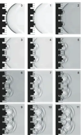
be di↵used temporally, or in respect to time as is shown for a transient wave in Figure

[image:21.595.221.419.122.233.2]

2.3.3. The rationale behind using acoustic di↵users to treat an acoustic space may be

Figure 2.3.2: Incident wave spatially di↵used

Figure 2.3.3: Cylindrical wave reflected from a Schroeder di↵user

cal-culated using an FDTD model. From Cox & D’Antonio p. 36 [7].

to reduce strong reflections, to reduce the e↵ect of comb filtering (discussed in Chapter

2.3.4), or provide a more even sound field [7]. Wenger Corporation [1] recommend

in-stalling acoustic di↵users in the front third of a performance space to help project sound

towards the audience, and Cox & D’Antonio [7] recommend sound di↵users on the rear

walls of performance spaces to avoid strong transient reflections. The di↵use properties

of a space can be assessed through a measurement of the sound field in di↵erent

loca-tions, and through measurement of the temporal response of a transient sound wave [7].

Two indicators of the performance of a di↵user are the scattering coefficient and the

[image:21.595.255.389.296.519.2]

(22)

to reduce the sound wave energy in the spatial reflection direction, whereas the di↵usion

coefficient is a measure of the uniformity of the spatial reflection across all directions [7].

2.3.3.1 Di↵usion coefficient

The di↵usion coefficient cdis a recent development in the characterisation of a surface’s

di↵usion properties, as published in the Audio Engineering Society (AES) standard

AES-4id-2001 (r2007) [3]. It is a single figure measure of the uniformity of scattering for a

surface at a particular frequency and incident angle. The AES standard states that the

di↵usion coefficient should be calculated as averaged one-third octave bandwidths to

smooth local variations [7]. The di↵usion coefficient is

cd, =

✓ _n

P i=1

10Li/10

◆2 _P_n

i=1

10Li/10 2

(n 1)Pn

i=1

10Li/10 2

(2.1)

wherenrepresents the number of receivers,Li the set of pressure levels in decibels from

the receivers and the source angle of incidence. The di↵usion coefficient can be

cal-culated in two or three dimensions and from experimental measurements or modelling,

provided each receiver position samples an area of the same size. [7]

While the di↵usion coefficientcn, provides a measure of the uniformity of scattering, it does not provide a measure of the increase in scattering when compared to a flat

surface. This is particularly important at low frequencies, where a flat surfaces can act

as a point source and provide high levels of di↵usion [7]. For this reason, the di↵usion

coefficient is normalised with reference to a flat surface of similar dimensions. The

normalised di↵usion coefficient cn, is defined as

cn, =

cd, cr,

1 cr,

(2.2)

where cd, is the di↵usion coefficient for the test sample, and cr, is the di↵usion

co-efficient for a reference flat surface of the same dimensions as the test sample, both

calculated using Equation (2.1).

The AES standard provides recommendations for the number of receivers, receiver

(23)

di↵usion modelling the standard recommends a source location of 5 m from the test

sample, and receivers at least every 5 around a 180 arc with radius 10 m from the test

sample. Unless otherwise stated, these AES recommendations will be followed in this

study for di↵usion modelling and calculation of the di↵usion coefficient, with the

excep-tion that receivers will be placed every 0.5 around the test sample. Negative values for

di↵usion coefficients are possible, in particular at low frequencies when a plane surface of

comparable size to wavelength exhibits high di↵usion properties. Cox & D’Antonio [7]

recommend displaying these as 0. However, they will be kept as negative values during

this work in the interest of data preservation and model comparisons.

0.8

0.6

0.4

0.2

0.0

100 2 3 4 5 6 7 8 91000 2 3 4 5

Frequency (Hz)

c_d - Diffusion coefficent

cn - Normalised diffusion coefficient

c_r - Reference diffusion coefficient

Figure 2.3.4: Comparison of cd,cp and cn for a N = 23 QRD. P = 2,

f0 = 500 Hz, N wT = 2.07 m, = 0 .

2.3.3.2 Scattering coefficient

Another coefficient used in the characterisation of di↵usion properties is the scattering

coefficient s. While the di↵usion coefficient is a measure of the uniformity of scattering,

the scattering coefficient is a measure of the ratio of energy reflected in the specular

reflection direction, to the total reflected energy. The scattering coefficient is published

in international standards number ISO 17497-1 [2], and can be represented as

s= 1 Espec

Etotal

, (2.3)

whereEspecis the energy di↵used in the specular direction, andEtotalis the total reflected

energy. The scattering coefficient value is averaged from all random incident angles and

(24)

noting that the total reflected energy does not include sound energy absorbed by the

material, expressed for an incident wave of unit energy as

Etotal= 1 ↵s,

and similarly, the specular reflected energy can be described as

Espec= (1 ↵s)(1 s),

where↵s is the absorption coefficient of the test sample.

The scattering coefficient is most commonly used when modelling reverberant fields

such as indoor acoustics through geometrical room modelling, and is therefore usually

calculated through experimentation at many incidence angles [11]. ISO 17497-1 describes

the method used for experimental calculating of the scattering coefficient.

The di↵usion coefficient is the most important parameter for di↵user design [11] and

is therefore the coefficient used in this work, but it is worth considering that both the

di↵usion coefficient and the scattering coefficient can be of use to describe the scattering

properties of a test sample.

2.3.4 Comb filtering

Comb filtering in acoustics is the e↵ect of certain frequencies becoming amplified, while

others are reduced, due to the interaction of a direct sound wave and its reflection from

a surface. The reflection causes a time delay of the direct sound due to the increased

distance it must travel, and when mixed with the direct sound can cause constructive

and destructive interference [11]. It is a feature of steady-state sources, and is generally

not considered for transient sound sources such as speech [11]. Occurring often due

to large flat reflective surfaces, it should be avoided in critical listening rooms such as

performance spaces and recording studios [7]. Treatment with absorbers and di↵users

can greatly reduce the e↵ect of comb filtering, where it may still occur but in a more

randomised manner [7]. Reducing the e↵ect of comb filtering can be a strong motive for

(25)

2.4 Acoustic di

↵

users

2.4.1 Development

There are many di↵erent of types of di↵users and di↵user purposes, including those

designed to scatter sound spatially or both spatially and temporally, as well as those

de-signed for three-dimensional di↵usion (commonly used on ceilings), and two-dimensional

di↵usion (commonly used on walls). The structural and architectural aspects of indoor

spaces will a↵ect their di↵usion characteristics, and certain features such as circular

pil-lars (see Chapter 2.4.2) can o↵er high di↵usion properties [11]. Di↵users can be installed

to further improve the di↵usion properties when needed. Di↵users are most commonly

rectangular panels with a surface profile designed to provide certain di↵usion

character-istics, but may also be convex shapes or other protruding geometries.

Manfred Schroeder is considered to have made the most substantial breakthrough

in di↵user design in 1975, when he presented his theory of reflection phase grating

dif-fusers [30],[25]. Schroeder di↵users o↵ered a key advantage in that their performance

could easily be predicted, and they are still considered amongst some of the the most

e↵ective di↵user designs used today. Schroeder di↵users are typically more efficient at

promoting di↵usion than many other protruding geometries such as rectangular, cubic,

triangular, polycylindrical and spherical shapes [11].

Recent advancements in computing power and the requirement for di↵users to fit

with modern architecture and interior design have led to surface profiles derived from

numerical optimisation. Numerically optimised di↵users may contain a hybrid of

ab-sorption and reflecting components, and surface profiles containing curved and square

edge components [7]. The pseudo-random profile of the di↵users is optimised through

computer modelling, and results may apply only to that particular size or application.

Unlike Schroeder di↵users which have known and repeatable di↵usion characteristics,

numerically optimised di↵users are designed for high performance only at the conditions

modelled during optimisation [6].

Di↵users with a surface profile described by two dimensions, such as an infinite

(26)

profile such as a sphere, are labelled two dimensional di↵users. Typically, one

dimen-sional di↵users scatter a sound wave two dimensions, and two dimensional di↵users

scatter a sound wave in three dimensions. The main focus of this work is one

dimen-sional Quadratic Residue Di↵users, though a background introduction will be given to

other common di↵user types.

2.4.2 Curved and cylindrical surfaces

A cylinder is an efficient two-dimensional di↵user [7]. With a simple design and shape

commonly found in architecture, the ability to model its behaviour is helpful to acoustic

space design. While sufficiently large cylinders have high quality di↵use properties,

their application as an acoustic treatment is limited by their size, as well as lack of

repeatability; a row of half cylinders along a wall do not have the same high standard

of di↵use properties [7]. Di↵raction from singular cylinders and spheres was modelled

analytically by Weiner [31], and the di↵raction from a set of half cylinders modelled using

the Boundary Element Method by Cox & D’Antonio [7]. The ability to analytically solve

di↵usion from a cylinder and sphere make them ideal test cases for BEM model validation

(see Chapter 5.2).

2.4.3 Schroeder di↵users

In two dimensions, Schroeder phase grating di↵users consist of wells of even width and

varying depth separated by thin panels. Di↵erent mathematical patterns govern the

depth of successive wells. Schroeder predicted that high levels of di↵usion could be

ob-tained through a surface profile of two di↵erent heights following the Maximum Length

Sequence (see Chapter 2.4.3.1) [25]. On top of this, Schroeder predicted that a phase

de-lay, or temporal di↵usion, could be obtained when the well depths follow certain patterns

such as the Quadratic Residue sequence (see Chapter 2.4.3.2) [26] and the Prime-Root

sequence (see Chapter 2.4.3.3) [11].

Schroeder di↵users are commonly used in repeating periods, where the di↵usion

ef-fects from a single period are enhanced by repetition. A period consists of N wells of

width w, separated by a thin panel of width w_P. The total width of a well and panel

is represented by wT, and consequently the period width is written as N wT, shown in

Figure 2.4.3a. One of the principles underpinning Schroeder di↵users is that the

(27)

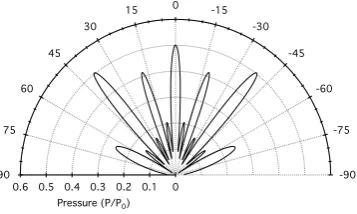
the polar di↵usion patterns, an example of which is shown in Figure 2.4.1. These lobes

are caused by the interference of delayed reflections from varying well depths, and give

Schroeder di↵users their high di↵usion properties. The number and strength of these

di↵usion lobes is governed by many factors including frequency and di↵user dimensions.

A design principle behind Schroeder’s theory of phase grating di↵users is that

longi-tudinal wave propagation within the wells dominates transverse waves. From this, the

upper frequency limit to the applicability of this theory can be stated as

min = 2w , (2.4)

where min is the minimum wavelength corresponding to the maximum frequency.

Be-yond this frequency, Schroeder di↵users may continue to display di↵usive properties but

they may be less e↵ective and consistent. The di↵usion performance of QRDs at

fre-quencies above this point is investigated in Part III of this work.

0 0.1 0.2 0.3 0.4 0.5

0.6 -90

-75 -60 -45 -30 -15 0 15 30 45

60

75

90

[image:27.595.227.406.395.502.2]

Pressure (P/P0)

Figure 2.4.1: Example of energy lobe di↵raction pattern fromN = 7

QRD at 4 timesf0. P = 3,N wT = 0.56 m,f0 = 500 Hz.

2.4.3.1 Maximum Length Sequence di↵users

Maximum Length Sequence (MLS) di↵users were the first type of reflection phase

grat-ing di↵user suggested by Schroeder in 1975 [25], and are the simplest form of Schroeder

di↵user. MLS di↵users are a one dimensional di↵user with even width sections of two

di↵erent heights. The height of each well is governed by the Maximum Length Sequence,

a pseudo-random binary sequence derived using maximal linear feedback shift registers.

Figure 2.4.2 shows an example of a MLS di↵user sequence. MLS di↵users are rarely used

because alternative Schroeder di↵users such as QRDs and PRDs o↵er superior di↵usion

(28)

Figure 2.4.2: Cross section of N=7 MLS di↵user. From Cox & D’Antonio p.296 [7].

2.4.3.2 Quadratic Residue Di↵users

The most popular Schroeder di↵user is the Quadratic Residue Di↵user (QRD). Similar

to MLS di↵users, QRDs consist of evenly spaced wells divided by thin panels. Well

depths are governed by the Quadratic Residue Sequence first studied by Gauss and

Legendre [26]. Thenth term in the sequence, sn, is defined as

sn=n2modulo(N), (2.5)

wheren= 0,1,2...(N 1), and modulo(N) represents the least non-negative remainder

when divided by a multiple ofN. The valueN is restricted to prime numbers, and also

represents the number of terms in each repeating sequence. In this way, the Quadratic

Residue Sequence is restricted to sequence lengths of 5, 7, 11... [25]. An exampleN = 7

quadratic residue sequence is calculated in Table 2.4.1, and a corresponding QRD is

pictured in Figure 2.4.3.

Table 2.4.1: Quadratic Residue Sequence calculation example forN =

7

n 0 1 2 3 4 5 6

n2 ₀ ₁ ₄ ₉ _{16 25 36}

n2_modulo(7) ₀ ₁ ₄ ₂ ₂ ₄ ₁

Schroeder used a Fourier transformation and representation of a QRD as a plane

surface with varying complex surface impedance (corresponding to well depths) to show

that QRD di↵usion patterns at design frequencies display lobes of even energy in di↵erent

angular directions [26]. The design frequency of a QRD,f0, is the lowest frequency at

(29)

scaling factor applied to all terms in the quadratic residue sequence when applied to a

QRD. Even energy lobes can be predicted at multiples of this design frequency. However,

between these frequencies QRDs can still display high di↵usion properties (see Part III).

The depth of welln,dn, in a quadratic residue di↵user for a design frequency of f0 and

prime numberN are determined from the equation

dn=

c

2N f0

sn, (2.6)

wherecis the speed of sound in air [25].

Another limiting factor of QRDs is the period widthN w_T. While even energy lobes

can be expected at the design frequency f0, if the period width is too small only one

energy lobe is present in the specular reflection direction, and the di↵user displays poor

di↵usion characteristics [7]. In Part III of this investigation, this e↵ect is reproduced

and the relationship between period width and lowest frequency of significant di↵usion

is investigated.

A feature of quadratic residue di↵users, and indeed of any Schroeder di↵user is their

ability to act as a plane surface at frequencies where all well depths are a multiple of

half the wavelength. The first frequency at which this will occur is termed the critical

frequency fc, and Schroeder di↵users can be expected to display very poor di↵usion

characteristics around this frequency [26]. For quadratic residue di↵users, the critical

-0.8 -0.6 -0.4 -0.2 0.0 0.2

(m)

-1.2 -1.0 -0.8 -0.6 -0.4 -0.2 0.0

(m)

w wP

dmax

Nw_T

(a)P = 1 (b)P = 3

(30)

frequency occurs where the first well depth is equal to half the critical frequency

wave-length c [7]. Using the relationship

c/2 =d1,

and combining with Equation (2.6),fccan be described in terms of the design frequency

as

fc =N f0. (2.7)

It can be seen from (2.7) that QRDs based on sequences with larger values ofN will have

a larger range between the design frequency and the critical frequency. It is suggested

by Cox & D’Antonio that the critical frequency should not be located within the desired

di↵usion bandwidth. [7]

Theoretically, the width of the well diving panels should be the minimum possible. It

is important however that they are thick enough to act as a rigid surface. An advantage

of modelling QRDs without using the thin panel method (see Chapter 2.5.2.1) is that

the e↵ect of varying well divider panel widths on di↵usion performance can be modelled,

and this is also investigated in Part III of this work.

The quadratic residue sequence as described by Equation (2.5) is naturally

asym-metrical. The first term s0 is 0, and the last term sN 1 is 1, independent of N. For

reasons of cost and desired symmetry, QRDs are often manufactured as a symmetrical

sequence, with the first well width halved, and an additional well of width w/2 and

depth 0 added at the end of the sequence. For installations of multiple QRD periods,

internal connections of well depth 0 have widthw, whereas the first and last wells of the

installation will have widthw/2.

The absorption of QRD panels is of interest to those designing acoustically critical

spaces. In many environments minimal absorption is desired, and QRDs are designed

accordingly. Three main variables a↵ect the absorption of QRDs: the relative width and

depth of wells; the build material; and the build quality. QRDs with long thin panels

can experience higher levels of absorption due to interaction of pressure waves and fluid

boundary layers along panels [7]. Wood is commonly used as a build material due to

(31)

Figure 2.4.4: N = 7 QRD array of multiple repeating periods. From

RPG Di↵usor Systems [10].

plastic, expanded polystyrene and sheet metal [7].

The build quality can have a large e↵ect on the absorption properties of a QRD.

Fujiwara & T. Miyajima [15] recorded absorption coefficients for QRDs between 0.3 and

1, in particular at frequencies below the design frequency. They later investigated these

high values of absorption and found that it was predominantly due to poor build

qual-ity and bonding of the QRDs tested [14]. Data from commercially available QRDs list

absorption coefficients between 0.2 and 0.3 [16].

2.4.3.3 Primitive Root Di↵users

Primitive Root Di↵users (PRDs) are very similar in design to QRDs in that they consist

of a series of wells of similar widths and varying depths. Well depths follow the Primitive

Root Sequence, defined as

sn=rnmodulo(N) (2.8)

forn= 1,2, ... N. sn is the nth term in the sequence,N is a chosen prime number and

r is the corresponding primitive root of N. The sequence has N 1 terms, and the

primitive rootr of any given prime number is one that allsnin the sequence are unique.

Primitive root values for their respective prime numbers can be found through trial and

error or are tabulated in Reference [12]. An example calculation of a Primitive Root

(32)

Table 2.4.2: Primitive root Sequence calculation example for N = 7,

r = 3.

Sequence number 1 2 3 4 5 6

rn ₃ ₉ _{27 81 243 729}

rn_modulo(_N₎ ₃ ₂ ₆ ₄ ₅ ₁

PRDs are designed to display the same even energy lobes as QRDs, as well as have

reduced di↵usion in the specular reflection direction. It is found that in the order

of 20 to 30 wells are needed to produce a noticeable reduction of reflected energy in

the specular reflection direction [7], and the frequency range in which it is occurs is

minimal [13]. PRDs generally have poorer di↵usion characteristics [7] and are also

inherently asymmetric, which is perhaps why QRDs are largely more popular than PRDs.

2.4.4 State-of-the-art on QRD design

2.4.4.1 Fractal di↵users

In an e↵ort to increase the optimum di↵usion frequency range for QRDs, panels at the

bottom of wells can be replaced by a smaller QRD with period width (N w_T)frac equal

to the larger QRD well width w. This is an e↵ective method for increasing di↵usion

at frequencies for which the larger QRD would otherwise become less e↵ective due to

transverse wave propagation within wells. Additionally, repeating periods of QRDs can

be installed with a varying datum following the quadratic residue sequence, which

as-sists in increased low frequency di↵usion, as well as reducing the e↵ect of undesirable

strong lobe concentrations [7]. An example of a commercially available fractal is the

QRD Di↵ractal, developed by D’Antonio & Konnert [9]. The Di↵ractal incorporates

three levels of fractals within its design and produces high di↵usion performance across

a wider bandwidth than standard QRDs. Fractals were shown to be an e↵ective way at

(33)

[image:33.595.252.389.77.343.2]

Figure 2.4.5: AnN = 7 QRD design with two levels of fractals. (Ever-est & Pohlmann p. 269 [11]).

2.4.4.2 Modulated QRDs

The quadratic residue sequence can be modulated so that thenth term, sn, is described

as

sn= (n2+k) modulo(N), (2.9)

where k is an integer constant. This introduces a constant phase shift to all terms in

the sequence. Table 2.4.3 shows the tabulated series for a regular Quadratic Residue

Sequence and modulated Quadratic Residue Sequence. In this example, the maximum

term number of the regular sequence is 12, and the maximum term for the phase shifted

sequence is 8. It follows from Equation (2.6) that the maximum depth of a QRD following

the phase shifted sequence will be 2/3 that of the regular sequence for a similar design

frequency. This can be useful in lowering the design frequency when depth constraints

are present, or in reducing losses in QRDs with narrow wells.

Table 2.4.3: Example of regular and phase shifted N = 13 Quadratic

Residue Sequence with value k= 4.

n 0 1 2 3 4 5 6 7 8 9 10 11 12

n2_modulo(_N₎ _{0 1 4 9 3 12 10 10 12 3 9} ₄ ₁

(34)

2.4.4.3 Three-dimensional Schroeder Di↵users

The application of the Quadratic Residue Sequence in di↵user design is not limited

to one-dimensional di↵users. The sequence can be e↵ectively layered on top of itself

in two di↵erent dimensions to produce a surface profile consisting of square wells of

di↵erent depths [11]. Two-dimensional Schroeder di↵users are capable of efficient

three-dimensional di↵usion often utilised to provide improved di↵usion from ceiling

reflec-tions [26].

(a) One-dimensional QRD _{(b) Two-dimensional QRD}

Figure 2.4.6: QRD and di↵usion pattern for one-dimensional and

two-dimensional QRDs. Adapted from Everest & Pohlmann p. 271 [11].

2.5 BEM

The Boundary Element Method (BEM) is a numerical method for solving the partial

dif-ferential equations that govern physical systems. It is used in the fields of stress analysis,

potential flow and acoustics [17]. In acoustic applications such as this work, the BEM

can be used to solve the Helmholtz equation for interactions between an incident acoustic

field and one or more surfaces within the field, and can be used to model acoustic fields

in both two and three dimensions. The BEM replaces the partial di↵erential equation

governing the domain solution with an equation governing the solution at the domain

boundary, and through surface discretisation and knowledge of the surface boundary

conditions, calculates a solution for the boundary acoustic potential (see Chapter 4.2).

From this solution the acoustic potential at any chosen point within the domain can

be calculated individually. The large advantage therefore with the BEM as compared

to Finite Element Analysis is a surface only requires discretisation, and a solution at

any point within any sized domain can be calculated without adverse implications for

(35)

domain of interest to be discretised, which reduces its practical application for large

domains or high frequencies that require small elements. The theory behind an acoustic

di↵usion implementation of the BEM is included in Chapter 4.

2.5.1 Conditions and Limitations

2.5.1.1 Continuous surface geometry

Using Green’s Second Identity (Eq. 4.5), the BEM computes a closed surface integral

around the object within the acoustic field [17]. Tests for this study encountered errors

when attempts were made to model an open surface with the BEM. Using the

regu-lar BEM, thin panels must be represented with a finite width, and errors can also be

encountered when thin panels are modelled without appropriately small elements (see

Chapter 5.2.5.1). A method called the thin panel solution exists for the representation of

thin panels as having infinitely small width, while still satisfying Greens Second Identity,

and avoids thin panel errors (see Chapter 2.5.2.1).

2.5.1.2 Non-unique solutions

When solving the simultaneous equations for surface pressures as part of the BEM, it

is possible to get non-unique solutions at certain frequencies which correspond to the

eigensolutions of the interior of the geometry being modelled. [7][17]. One of multiple

solutions to this problem is the CHIEF method. The CHIEF method adds an additional

constraint to the solution by requiring the pressure at one or more receivers within the

geometry surface to equal 0, which is satisfied only for correct solutions. The exception

to this is that internal receivers may be unknowingly placed at nodes of the incorrect

internal eigensolution where the pressure is 0. Seybert & Rengarajan [27] showed it is

generally a very e↵ective method at avoiding the problem of non-unique BEM solutions.

Cox & D’Antonio however state that it is rarely encountered when modelling acoustic

di↵users.

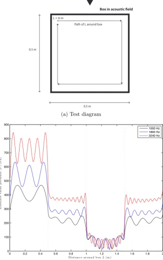
A simple but less efficient method of checking whether a BEM solution is a result

of non-unique solutions error was developed in the BEM code during this work, and is

(36)

2.5.2 State-of-the-art on BEM modelling

2.5.2.1 Thin panel solution to BEM modelling

When using the BEM to model geometry that contains thin panels or surfaces, errors are

sometimes encountered due to the proximity of front and back elements [7]. Terai [29]

published a solution to this in which a thin panel is represented as having infinitesimal

thickness and modelled as a surface instead of a closed boundary, and results in a

solu-tion for pressure on the front and back of these surface elements. Wu [32] took this thin

panel solution further, and developed a method to integrate it with the regular BEM

method so that a combination of the regular BEM and thin panel solution BEM can be

used together. While o↵ering a solution to the errors caused by thin panels in geometry

such as QRDs, it also reduces the number of elements needed and decreases computation

times.

The need for the thin panel solution has arguably decreased as computation power

has increased. In 1994, Cox & Lam [8] noted a running time of 10 hours for a BEM model

of a QRD consisting of 768 elements at one frequency. Element sizes small enough to

model thin panels without errors were not possible, so the alternative to the thin panel

solution was a ‘box model’ with varying complex surface impedance to represent the

phase delay of QRD wells, thereby neglecting the e↵ects of any non-longitudinal wave

propagation within wells. The thin panel solution therefore provided a strong advantage

over other methods at the time. With the increase in computer storage and computing

power today, as well as methods to increase efficiency of meshing and computation (see

Chapter 5.2) BEM models are much faster.

The BEM program developed in this work takes approximately 13 seconds for a

similar QRD model of 768 elements (see Chapter 5.2.6). The element length needed to

avoid thin panel errors was also investigated in Chapter 5.2.5.1, and it is shown that

element sizes needed to avoid thin panel errors are achievable with reasonable running

times. Using this, the BEM model accurately represents a QRD including thin panel

(37)

2.5.2.2 Three dimensional modelling with the BEM

While the focus of this study is the application of the BEM in two-dimensions, it is

also an e↵ective method of modelling in three dimensions. Three-dimensional modelling

requires particular attention to the geometry discretisation, where elements must be

represented by small flat panels, instead of straight lines for the two-dimensional case,

and this is where human error will most likely occur [7].

The BEM in three-dimensions is useful tool to model surface profiles that vary in

three dimensions, such as a sphere or two-dimensional QRD. However, Cox & Lam [8]

showed the two-dimensional BEM is accurate in predicting the di↵usion patterns of

one-dimensional di↵users, and the additional computation time necessary for

[image:37.595.227.409.340.454.2]

three-dimensional modelling is not necessary.

Figure 2.5.1: A two-dimensional di↵user modelled using a

(38)

Part II

BEM Code Development and

(39)

Chapter 3 MATLAB BEM Overview

Part I of this work is the further development and optimisation of a MATLAB

imple-mentation of the BEM. The theory used in gaining a solution using the BEM is derived

in detail (Chapter 4). Significant changes and developments to the code are documented

(Chapter 5), including methods to increase the solution speed and accuracy. The BEM

code is then tested in comparison to an analytical solution (Chapter 5.2.2), published

results (Chapter 5.2.3) and the original BEM code (Chapter 5.2.6). A detailed accuracy

study is also conducted with reference to model geometry, frequency and element size,

from which recommendations are made for the appropriate use of the code when

mod-elling Schroeder di↵users (Chapter 5.2.5).

A brief description of executing the BEM code, and major MATLAB functions within

the code is given (Chapter 3.2). A tabulated breakdown of the program steps used in the

BEM is described in Appendix B.1. A flowchart shows the MATLAB functions used in

the calculation of di↵erent variables, including acoustic field types and frequency bands

(Chapter 3.2.1).

3.1 Acknowledgements

This work is a continuation of the works of Luca Rocchi [23] and Nick Smith [28], who in

2013 implemented the BEM into a MATLAB function and validated its accuracy against

both published literature and Finite Element Analysis models. Some sections of code

are completely re-written while others are largely untouched. A guide to the author of

sections is given in the individual function comments. Credit should be given to Rocchi

(40)

3.2 Executing the BEM code

The BEM code can be executed from the MATLAB function run_BEM . All test

pa-rameters can be assigned values within this function, and it includes geometry creation

functions for most common QRD designs and modifications. run_BEM can be modified

to return output results as necessary.

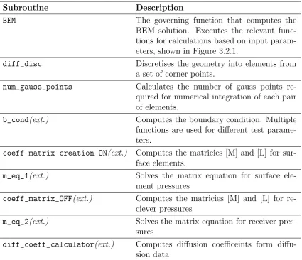
run_BEM executes multiple subroutines as part of obtaining a solution. A summary

of major subroutines is included in Table 3.2.1. (ext.) indicates multiple version of the

code exist with di↵erent names for di↵erent input parameters, such as frequency band

averages and incident acoustic source types. Many other subroutines are involved in

geometry creation and minor calculations, and are described in the relevant function

[image:40.595.110.536.365.731.2]

comments.

Table 3.2.1: BEM code subroutines

Subroutine Description

BEM The governing function that computes the

BEM solution. Executes the relevant func-tions for calculafunc-tions based on input param-eters, shown in Figure 3.2.1.

diff_disc Discretises the geometry into elements from

a set of corner points.

num_gauss_points Calculates the number of gauss points re-quired for numerical integration of each pair of elements.

b_cond(ext.) Computes the boundary condition. Multiple functions are used for di↵erent test parame-ters.

coeff_matrix_creation_ON(ext.) Computes the matricies [M] and [L] for sur-face elements.

m_eq_1(ext.) Solves the matrix equation for surface ele-ment pressures

coeff_matrix_OFF(ext.) Computes the matricies [M] and [L] for re-ciever pressures

m_eq_2(ext.) Solves the matrix equation for receiver pres-sures

(41)

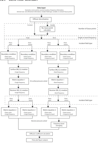
3.2.1 BEM code flowchart

Data input

Geometry corner points, receiver locations, frequency information,

element size and refinement information, incident field type, variable or constant Gauss points.

Diffuser discretisation

No. Gauss point

calculator Number of Gauss points

Variable Constant

Single or band frequency

Incident field type

Single Band

Plane

wave PointSource Planewave Point source

Boundary condition Boundary condition Boundary condition Boundary condition

t1MBOFXBWF

t4JOHMFGSFRVFODZ t1PJOUTPVSDFt4JOHMFGSFRVFODZ t1MBOFXBWFt'SFRVFODZCBOE t1PJOUTPVSDFt'SFRVFODZCBOE

Surface [M], [L] creation

t4JOHMFGSFRVFODZ t#BOEGSFRVFODZ

Matrix equation 1

t4JOHMFGSFRVFODZ

Matrix equation 1

t#BOEGSFRVFODZ

Receiver [M], [L] creation Receiver [M], [L] creation

On surface pressures solved

t4JOHMFGSFRVFODZ t#BOEGSFRVFODZ

Plane

wave PointSource Planewave Point source

Matrix equation 2

t1MBOFXBWF t4JOHMFGSFRVFODZ

Incident field type

Matrix equation 2

t1PJOUTPVSDF t'SFRVFODZCBOE

Matrix equation 2

t1MBOFXBWF t'SFRVFODZCBOE

Matrix equation 2

t1PJOUTPVSDF t4JOHMFGSFRVFODZ

Reciever pressures solved

'SFRVFODZCBOE

averaging

Diffusion coefficient calculation

Polar plot figure outputs

[image:41.595.112.520.112.706.2]

Surface [M], [L] creation

(42)

Chapter 4 BEM Theory

4.1 BEM assumptions

During this implementation of the BEM for acoustic modelling, the following

assump-tions are made:

1. The surface is rigid and acts as a perfect reflector, with no sound absorption

or transmission through the geometry medium. It is possible to apply a surface

impedance to simulate absorption. However, the e↵ectiveness of this for Schroeder

di↵users may be questioned, in particular at lower frequencies, as research shows

factors such as build quality and panel bonding techniques can a↵ect absorption

as much as the build material (see Chapter 2.4.3.2).

2. The acoustic field is a combination of the incident field and modelled surface

reflections only. The domain is considered infinite or as having a boundary with

an absorption coefficient ↵= 1.

3. The domain is an isotropic homogeneous fluid. Pressure wave energy losses due

to viscous e↵ects are negligible, and may be ignored.

The above assumptions are reasonable for acoustic modelling of di↵user geometries in

room temperature air within the approximate range of 100 - 7000 Hz. Assumption 1

holds well for most rigid di↵users, particularly as most commercial products are designed

for minimal absorption (see Chapter 2.4.3.2). Assumption 2 is a simplification made for

the purpose of modelling and performance characterisation. While incident waves may

be dominant for many di↵user applications, the sound field will consist of an incident

wave together with reflections from other surfaces including walls and floors. A transient

wave can accurately replicate an infinite boundary within the time taken for first order

reflections from other surfaces to reach a receiver, as done by Cox & D’Antonio [7].

(43)

distances, or in media with high viscosity, where attenuation from viscous energy losses

must be taken into account.

4.2 Wave theory

A sound field of periodic waves can be represented by a potential function (p), where

pis an arbitrary point within the domain1, and (p) satisfies the Helmholtz equation

r2 +k2 = 0, (4.1)

wherekis the wavenumber, representing the number of cycles per unit distancek= 2⇡f ,

f represents frequency (Hz), and represents the wave phase velocity (m/s). The wave

potential function (p) describes the pressureP at any pointp, as:

P = ⇢@

@t =i⇢! , (4.2)

V =r . (4.3)

BothP and are assumed to be sinusoidal, and are represented as complex variables, in

which absolute value represents magnitude and argument represents relative phase. For

an open sound field, we can write the sound field as the superposition of the incident

and di↵racted sound fields

total = incident+ di↵racted. (4.4)

From here onwards, the subscripts T, I and D represent total, incident and di↵racted

respectively. From (Eq. 4.3) we can extend this to superposition of the incident and

di↵racted acoustic wave velocity

VT =VI+VD. (4.5)

4.3 Incident sound field

When modelling di↵usion in two dimensions, there are two obvious choices for an incident

sound field: that of a incident plane wave, and that of a point source located at some

(44)

point in the external domain. For the purpose of a BEM analysis, the incident sound

field must be modelled at a snapshot in time, in which time is constant and pressure is

a function of position only. For the case of an incident plane wave, takes the form

= oe ikx, (4.6)

where

@

@x = ik 0e

ikx_,

@

@y =

@

@z = 0.

A point source incident sound field can be represented by the Hankel function as

=H₀(1)(kr), (4.7)

and from Chapter 4.7,

d drH

(1)

0 (kr) = kH

(1) 1 (kr),

where r is the magnitude of the vector between the point source and receiver. The

Hankel function is undefined at a value ofkr= 0 (see Chapter 4.7). However, it can be

scaled by a constant as needed to interpret results.

4.4 Rigid body boundary condition

The implementation of the Boundary Element Method requires knowledge of the

bound-ary conditions along a surface. During this investigation, it is assumed that the surface

is perfect reflector, expressed mathematically asVT·nˆ = 0, wherenˆ is the unit outward

normal vector from any point on the boundary. Using this result we can reduce equation

(Eq. 4.5) to

VD ·nˆ = VI ·nˆ,

and combined with (Eq. 4.3), this becomes

@ D

@nˆ = VI ·nˆ. (4.8)

(45)

4.5 Green’s second identity

Green’s Second Identity, derived from the divergence theorem, can be written as

‹ ✓

(q)@G(p,q)

@nq

G(p,q) @

@nq

◆

dSq = C (p), (4.9)

whereG(p,q) represents the e↵ect of a unit source atqon a pointp. From the definition

ofG given in (Eq. B.10), the coefficient C has values of:

• 0 for points not within the domain;

• 0.5 for points that lie on the boundary; and

• 1 for points within the boundary.

Substituting in the Rigid Body Boundary Condition (Eq. 4.8) gives

‹ ✓

(q)@G(p,q)

@nq

( VI ·nˆq)G(p,q) ◆

dSq= C (p), (4.10)

This is an important result, and is the basis of the Boundary Element method. It

allows the sound potential at any point on the surface (p) to be written in terms of the

surface geometry and the incident sound field. A derivation of Green’s second identity

from the divergence theorem is shown in Appendix B.2.

4.6 Discretisation of the boundary

To apply the Boundary Element Method to any arbitrary surface, it must first be

dis-cretised into a number of small segments, with the assumption that is constant across

that section.

This assumption enables us to describe Green’s Second Identity (Eq. 4.9) for any

element i in a discretised form as

C i= n X

j=1 j

ˆ qj

qj 1

(_rG_·nˆj) dS+ (V ·nˆj) ˆ qj

qj 1 GdS

(46)

or using simplified notation

C i= n X

j=1

( jMij+ (V ·nˆj)Lij) , (4.11)

where

Mij =

ˆ qj

qj 1

rG(pi, qj)·nˆdS , (4.12)

Lij = ˆ qj

qj 1

G(pi, qj) dS . (4.13)

Substituting in C = 1₂, (Eq. 4.11) can be written in terms of a vector of all surface

potential values{ } as

1

2[I]{ }= [M]{ }+ [L]{VI ·nˆ} (4.14)

and combining the two{ } terms,

[L]_{VI ·nˆ}= ✓

[M] + 1

2[I] ◆

{ }. (4.15)

(Eq. 4.15) can be used to solve for the vector of surface potential values _{ surf}. O↵

surface potential can be solved through substituting this into the right hand side of

(Eq. 4.14), and replacing the left hand side with_{ o↵-surf}.

4.7 The Hankel functions

So far, the sound field intensity at each point on a surface has been described using a

function that relates the e↵ect of a unit source at pointq has on pointp;G(p,q). This function must satisfy the Helmholtz equation (Eq. 4.1). For two-dimensional waves, this

function can be represented by the Hankel functions of the first kind and order zero as

published by Abramowitz and Stegun [4]:

H_⌫(1)(z) =J⌫(z) +iY⌫(z), (4.16)

and

(47)

whereJ⌫(z) and Y⌫ the Bessel functions of the first and second kind respectively, both

of order⌫,r is the magnitude of the distance betweenpandq, and↵ is a constant. The

Hankel functions are chosen because they satisfy the Helmholtz equation in cylindrical

coordinates.

To calculate the coefficient ↵, we recall that in the derivation of Green’s Second

Theorem (Appex. B.2), the functionG(p,q) was scaled so that

@G

@r =

1

2⇡r as r!0. (4.17)

From Abramowitz and Stegun [4],

iH₀(1)(z)_⇠ 2

⇡ln(z) as z!0,

hence

d dzH

(1)

0 (z)⇠

2i

⇡z as z!0. (4.18)

Combining (Eq. 4.17) and (Eq. 4.18) to solve for↵,

dG(kr)

dr =k

dG(kr)

d(kr) !kC 2i

⇡kr =

1

2⇡r asr !0,

and

↵= i

4. (4.19)

Abramowitz and Stegun [4](Ch. 9.1.28) also state the relationship

Y_o0(z) = Y1(z), J00(z) = J1(z) as z!0

and from (Eq. 4.16) it follows that

d d(kr)H

(1)

0 (kr) = H

(1)

1 (kr), (4.20)

and

d drH

(1)

0 (kr) = kH

(1)

1 (kr). (4.21)

(48)

10−2 10−1 100 101 0 5 10 15 20 25 30

Dis t anc er

f(r)

H anke l f unc t ions of t he fir s t k ind, z e r ot h andfir s t or de r .

H0( 1 )

[image:48.595.138.489.79.317.2]

H1( 1 )

Figure 4.7.1: Absolute value of Hankel functions of constant k and

increasing r.

equations used to model the e↵ect of a unit source on a point:

G(p,q) = i

4H

(1)

0 (kr), (4.22)

@G(p,q)

@nˆ =

ik

4H

(1)

1 (kr). (4.23)

For any given wavenumber, these functions decrease with an increase inr as shown in

Figure 4.7.1.

From equation (Eq. 4.23),

rG(p,q)·nˆq =

ik

4H

(1)

1 (kr)(ˆr·nˆq), (4.24)

and using this result, the coefficient matrices [L] and [M] become

Lij = ˆ qj

qj 1 i

4H

(1)

0 (kr) dS (4.25)

Mij = ˆ qj

qj 1 ik

4H

(1)

1 (kr)(ˆr·nˆj) dS . (4.26)

It will be seen in Chapter 4.8 that these integrals can be computed numerically and in

(49)

can be solved to find the surface potential for a given incident sound wave.

4.8 Integration methods

4.8.1 Numerical integration

The values of the coefficient matrices [L] (Eq. 4.13) and [M] (Eq. 4.12) can be

com-puted by any number of numerical integration techniques. Due to the free choice of

sample points available, the Gaussian Quadrature Integration technique was chosen as

it provides the highest order of accuracy for a given number of points, and is easily

im-plemented. Numerical results from the Hankel functions (Eq. 4.22) and (Eq. 4.23) can

be computed easily by numerical programs such as MATLAB using in-built functions.

The general form of Gaussian Quadrature integration is (from Kreyszig [18])

ˆ b

1

f(x)dx_⇡ ✓

a+b

2

◆_Xn

j=1

wjf(xj) +Rn,

where xj is a set of sample point locations, each with a corresponding weighting wj.

Sample locations and weights used have been published by Abramowitz and Stegun [4]

and are listed in Appendix B.5. For a number of gaussian points n, the coefficient

matrices [L] and [M] are calculated as

Lij =

(qj qj 1) 2 i 4 n X m=1

wmH0(1)(krm) (4.27)

Mij =

(qj qj 1) 2 ik 4 n X m=1

wmH1(1)(krm)(ˆr·nˆj). (4.28)

A notable property of the Hankel functions (Eq. 4.22) and (Eq. 4.23) is

lim z!0H

(1)

0 (z) =1, and

lim z!0H

(1)

1 (z) =1,

as shown in Figure 4.7.1. Due to this result, evaluating the Hankel function at the source

location (r = 0) must be avoided. Rocchi [23] and Smith [28] avoided this problem

through using an even number number of quadrature points across the element in order

Development of a 2D boundary element method to model Schroeder acoustic diffusers