City, University of London Institutional Repository
Citation
:
Valani, Y.P. (2011). On the partition function for the three-dimensional Ising
model. (Unpublished Doctoral thesis, City University London)
This is the accepted version of the paper.
This version of the publication may differ from the final published
version.
Permanent repository link: http://openaccess.city.ac.uk/7793/
Link to published version
:
Copyright and reuse:
City Research Online aims to make research
outputs of City, University of London available to a wider audience.
Copyright and Moral Rights remain with the author(s) and/or copyright
holders. URLs from City Research Online may be freely distributed and
linked to.
City Research Online:
http://openaccess.city.ac.uk/
[email protected]
On the partition function for the three-dimensional Ising
model
Yogendra P. Valani
A thesis submitted for the degree of
Doctor of Philosophy of City University London
City University London,
School of Engineering and Mathematical Sciences,
Northampton Square,
London EC1V 0HB,
United Kingdom
August 2011
The candidate confirms that the work submitted is his own and that appropriate credit has been
given where reference has been made to the work of others. This copy has been supplied on the
understanding that it is copyright material and that no quotation from the thesis may be
Contents
Table of Contents . . . ii
List of Figures . . . v
List of Tables . . . viii
Dedication . . . ix
Dedication . . . x
Acknowledgements . . . xi
Abstract . . . xii
1 Introduction 1 1.1 Physics background . . . 1
1.1.1 Statistical Mechanics . . . 2
1.1.2 Partition functions . . . 2
1.1.3 Observables . . . 3
1.1.4 Potts models . . . 5
1.2 Known results . . . 6
1.2.1 Two-dimensional Ising model . . . 6
1.2.2 Perturbation expansions . . . 7
1.2.3 Duality . . . 10
1.2.4 Monte-Carlo methods . . . 14
1.2.5 Existing exact finite lattice results . . . 16
1.3 Physical interpretation of results . . . 16
1.4 Universality . . . 17
2 Computational Method 18 2.1 Potts models on graphs . . . 18
2.2 Partition vectors and transfer matrices . . . 20
2.2.1 Transfer matrices . . . 23
2.2.2 Geometry and Crystal lattices . . . 25
2.2.3 Eigenvalues of the transfer matrix . . . 26
2.3 Zeros of the partition function . . . 28
2.3.2 Eigenvalues and the zeros distribution . . . 29
2.4 Correlation functions . . . 31
3 Potts model partition functions: Exact Results 34 3.1 On phase transitions in 3d Ising model . . . 37
3.2 Validating our interpretation of results . . . 42
3.2.1 Checking dependence on boundary conditions . . . 45
3.2.2 Checking dependence on size . . . 52
3.3 Further analysis: Specific heat . . . 54
3.4 Eigenvalue analysis . . . 60
3.5 Q-state: 2d Potts models (Q >2) . . . 62
3.6 Q-state: 3d Potts models (Q >2) . . . 64
4 Discussion 68 A Onsager’s Exact Solution proof 70 A.1 Notations and background maths . . . 70
A.1.1 Matrix algebra . . . 70
A.1.2 Clifford algebra . . . 71
A.2 Rotational matrices . . . 73
A.2.1 Rotations in 2n-dimensions . . . 73
A.2.2 Rotational matrices and Clifford algebra . . . 73
A.2.3 Product of rotational matrices . . . 75
A.2.4 Eigenvalues of W . . . 77
A.3 Formulation . . . 78
A.3.1 Local transfer matrices . . . 78
A.3.2 Local transfer matrices and gamma matrices . . . 81
A.3.3 Rotational and transfer matrices . . . 82
A.3.4 Eigenvalues ofS(W) . . . 85
A.3.5 The indeterminate solution . . . 85
A.3.6 Thermodynamic limit solution . . . 86
B Code 87 B.1 Hamiltonian symmetries . . . 87
B.2 Transfer matrix symmetries . . . 89
B.2.1 Spin configurations . . . 91
B.3 Large numbers, memory . . . 91
C Checking results 93
E Example of exact partition function 97
List of Figures
1.1 Specific heat of the two dimensional Ising model . . . 7
1.2 Showing the low temperature expansion for part of a 2d lattice. Full circles denote spins pointing up, and open circles are spins pointing down. . . 8
1.3 Showing the high temperature expansion for part of a 2d lattice. Full circles denote spins pointing up, and open circles are spins pointing down. . . 9
1.4 Dual triangular and honeycomb lattice . . . 11
1.5 A graphG (black vertices and solid lines) representing a 4×4 lattice, and its dual lattice (white vertices and dashed lines). . . 11
1.6 An example of a mapping between graphG′⊂ G(black vertices and solid lines) and a dual ofG,D′ ⊂ D(white vertices and dashed lines). . . 13
1.7 Various zeros of a 2d Potts model withQ= 2 fixed on graphsGandDfrom Figure 1.5. The solid cross represents the unit axis of the complex temperature plane. . . 15
2.1 A planar realisation of an undirected graphG. . . 19
2.2 Shows setV ⊆VG. . . 20
2.3 GraphsG andG′ . . . . 22
2.4 The resultant graphGG′, obtained by combining G andG′ (from Figure 2.3) overV. 22 2.5 A graphical example of Lemma 2.2.4 . . . 22
2.6 Representing incoming and outgoing spins usingI andE respectively . . . 23
2.7 Binding graphs, and spin categories . . . 24
2.8 Showing d-dimensional lattices. The grey spin in each figure, represents a typical bulk spin and its nearest neighbour interactions (red edges). . . 25
2.9 Examples ofd-dimensional transfer matrix lattice layers. Incoming (outgoing) spins are modelled by grey (white) vertices . . . 26
2.10 The zeros of Tr(T100) (red dots) and the zeros ofB(x) (blue crosses). . . . 31
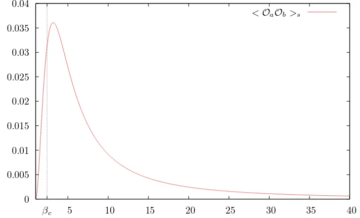
2.11 A 2×3 lattice, with sites labelledaandb. The white site is a fixed spin. . . 33
2.12 A plot of <OaOb>s againstβ for the Ising model on a 2×3 lattice. . . 33
3.1 Evidence of a critical point in 3d Ising model? . . . 35
3.2 The zero distribution for a 10×10 (self dual) lattice. . . 36
3.4 With reference to Figure 3.3: (a) overlays the zeros distributions close toF in the
first quadrant; (b) overlays the corresponding specific heat curves. . . 39
3.5 With reference to Figure 3.1: (a) overlays the zeros distributions close toF in the first quadrant; (b) overlays the corresponding specific heat curves. . . 41
3.6 Graphs of tanh(βNi), where N1< N2< N3 . . . 42
3.7 Boundary interactions . . . 43
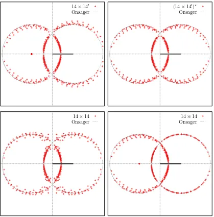
3.8 Zeros of the partition function Z in x for the 14×14 Ising model with various boundary conditions. . . 45
3.9 Zeros of Z in x for the Nx×Ny′ Ising model with fixed open/periodic boundary conditions. . . 46
3.10 Zeros of Z in xfor the 5×5×N′ z Ising model. . . 47
3.11 A configuration of the Ising model on a 3×4 lattice. . . 48
3.12 Control boundary conditions I . . . 49
3.13 Control boundary conditions II . . . 50
3.14 Control boundary conditions III . . . 51
3.15 Showing the zeros ofZ =xN + 1, for variousN . . . . 52
3.16 Control:lattice size I . . . 53
3.17 Control lattice size II. . . 54
3.18 With reference to Figure 3.8: (a) overlays the zeros distributions close to F in the first quadrant; (b) overlays the corresponding specific heat curves. . . 55
3.19 Overlay and specific heat of Figure 3.12 . . . 56
3.20 Overlay and specific heat of Figure 3.16 . . . 56
3.21 Overlay and specific heat of Figure 3.14 . . . 57
3.22 Overlay and specific heat of Figure 3.17 . . . 57
3.23 An overlay of zero distributions of large lattices close toF, along with their corre-sponding specific heat curves. . . 58
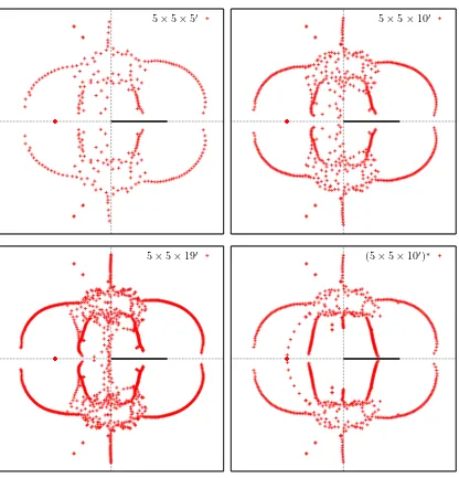
3.24 A look at the 5×5×Nz on various axis. . . 59
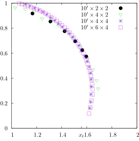
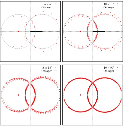
3.25 Zeros of the partition functionZ for the 10×Ny Ising model,Ny={10′,20′,50′,99′}. 60 3.26 Zeros of the partition functionZ inx=eβ. . . . 61
3.27 The zeros of the partition functions inZ inx=eβ for variousQ= 3-state 2d Potts models . . . 62
3.28 The zeros of the partition functions inZ in x = eβ for various (Q > 2)-state 2d Potts model . . . 63
3.29 The zeros of the partition functions in Z in x =eβ for (Q = 3)-state models on various 3d lattices. . . 65
3.30 The zeros of the partition functions in Z in x=eβ for (Q= 3)-state models on a 3×4×10′ lattice with various boundary conditions. . . . . 66
A.1 Adding a sequence of horizontal and vertical bonds to a lattice . . . 79
B.1 Showing two possible routes that an extra layer is added to the 4×4×Llattice (1). The resultant is a 4×4×(L+ 1) lattice (2). . . 88
B.2 The spins on a layer of 4×4×L lattice are organised into columns and the sets labelledV1, . . . , V4 . . . 90
B.3 Examples of local transfer matrices . . . 90
B.4 A transfer matrix used in the code . . . 90
List of Tables
3.1 Table of Potts model partition functions, for exact finite lattice presented in this
chapter. . . 37
4.1 Extrapolating the critical point, using various curve fitting techniques. . . 68
Acknowledgement
I would like to express immense thanks to my primary supervisor, Prof. Paul Martin. This research
and thesis would not be possible without him. I am very grateful to have had such a friendly and
helpful supervisor. Thank you for all your advice, support, patience and encouragement. For all
supervisions (in person, on the phone, via email, skype, and the web forum, etc...), and for the
day long supervisions. I would also like to extend my thanks to Paul’s family, Paula, Laura and
Hannah Martin, for their hospitality during my visits to Leeds.
To my wife Selina, who I met in the first year of my research, I would like to thank for all her
support and encouragement throughout. For the endless hours you have spent listening to me. For
picking me up, every time I want to give up, and for never letting me give up. I don’t know how
I would have come this far without you. I am eternally grateful for all the sacrifices you have had
to make, especially over the last 6 months.
To all my wonderful family and friends who have supported and believed in me, thank you for
being there. I am very fortunate to have a close network of friends who have always been there.
For the times when I have had enough and needed some time out, my friends have always been
there.
Thank you to my examiners Prof. Uwe Grimm and Prof. Joe Chuang for many useful comments
and corrections. I also like to extend my thanks to staff at City University for all their help.
Thanks to Dr. Anton Cox my second supervisor. A big thank you to Dr. Maud De Visscher for
proofreading and organising funding for my supervisions in Leeds. Also thanks to the IT dept. at
City University, in particular Chris Marshall, Jim Hooker, and Ferdie Carty. I would like to thank
course officers Sujatha Alexandra and Choy Man, for sorting out countless problems.
There have been a few times during the research, that due to financial difficulties I would not
have been able to complete my research. I am indebted to my parents; my wife; siblings Ramnik
Valani and Khyati Savani; Jeegar Jagani; Nimesh Depala; Manish and Diptiben Depala, for making
it possible for me to continue.
Thanks to Zoe Gumm for proofreading and organising a write-up plan. For many useful physics
discussions I am grateful to E. Levi, A. Cavaglia, C. Zhang, E. Banjo. Thanks to M. Patel and J.
Jagani for the insightful discussion on statistics and Monte–Carlo techniques.
Finally, a very special thanks to my parents, Pravin and Vasanti Valani, for all their support
Abstract
Our aim is to investigate the critical behaviour of lattice spin models such as the three-dimensional
Ising model in the thermodynamic limit. The exact partition functions (typically summed over
the order of 1075 states) for finite simple cubic Ising lattices are computed using a transfer matrix
approach. Q-state Potts model partition functions on two- and three-dimensional lattices are
also computed and analysed. Our results are analysed as distributions of zeros of the partition
function in the complex-temperature plane. We then look at sequences of such distributions for
sequences of lattices approaching the thermodynamic limit. For a controlled comparison, we show
how a sequence of zero distributions for finite 2d Ising lattices tends to Onsager’s thermodynamic
solution. Via such comparisons, we find evidence to suggest, for example, a thermodynamic limit
Chapter 1
Introduction
1.1
Physics background
This thesis is a study of the analytic properties of certain models of co-operative phenomena
(cf. [102, 89, 57]). A physical system exhibits a co-operative phenomenon if there is a coherent
relationship between its microscopic constituents leading to macroscopic properties.
A ferromagnet [79, §7.3] is an example of such a system, as there is a coherent relationship
between its magnetic dipoles leading to a bulk magnetisation [49].
[1.1] To compare macroscopic properties of a physical system we categorise the system state into phases [7]. For example, at low (high) temperature a ferromagnet is said to be in a ferromagnetic
(paramagnetic) phase, if it has (does not have) a bulk magnetisation. We can move from one phase
to another by adjusting its temperature T (the mechanism for this will be discussed later). We
shall only focus on systems (such as the ferromagnet) where phase changes only occur at a definite
point. The point at which the phases co-exist is known as thecritical point. At the critical point
the system is said to be undergoing a phase transition [89, 27].
Physical experiments on a system can tell us what its critical point is. For example, a well
known critical point is the Curie temperatureTc (whereTc= 1043K for iron [11,§1.1]), at which
spontaneous magnetisation [5] vanishes (cf. Baxter (1982) [9, §1.1]). See Binney et al (1992) [11,
§1.6] and references therein for several other examples.
[1.2]The Curie temperature categorises a ferromagnet as being in: the disordered (paramagnetic) phase whenT > Tc; the ordered (ferromagnetic) phase whenT < Tc; and a phase transition when
T =Tc.
We describe this transition (known as the order/disorder transition) as follows [37]. In the
ferromagnetic phase, magnetic dipoles are not randomly orientated but are aligned parallel (even
in the absence of an external field) to give a net magnetisation. This is known as spontaneous
magnetisation. Here we denote the net magnetisation byM. AsT is increased1(ie. by adding heat
energy to the system) the orientation of one or more dipoles may fluctuate and become unaligned
1
from the ordered state. As a result M will decrease. Then at T = Tc we see that M suddenly
drops to zero, and remains zero for all T > Tc. The magnet has changed to the paramagnetic
phase.
We usestatistical mechanicsto investigate phenomena such as the Curie point phase transition.
1.1.1
Statistical Mechanics
Classic mechanical theory does well in following a particle through a force field [7]. It even extends
to a many-body system [53, §11]. However, there are typically 6×10
23 (Avogadro’s number)
particles [13] in a real world system. Using Newtonian mechanics on this scale would be impossible
computationally. On the other hand, thermodynamics [16, 40] is a theory used to observe data for
systems on a macroscopic scale. This theory gives results on a macroscopic level, and yet fails to
answer how transitions occur between phases [91].
[1.3]Statistical mechanics[9, 40, 44, 67, 69] is a theory that attempts to “bridge” the gap between microscopic entities and macroscopic observables. It attempts to predict the macroscopic behaviour
of a physical system (or process), by analysing its microscopic components.
In this thesis, we focus onequilibrium statistical mechanics [44]. When the state of the system
is independent of time we say the system is in equilibrium [20]. As an example, consider a hot
cup of coffee in a room. As the coffee cools it is not in equilibrium. However when it is at room
temperature, the coffee will have the same temperature regardless of whether we observe it over a
few minutes or over a few hours. Here we say the system is in equilibrium.
As real world systems/phenomena are far too complex to accurately investigate mathematically,
a simplistic model that extracts only the essential features is employed [50]. The aim of this model
is to predict the results of an unobserved (but suitably nearby) regime. In this thesis, we shall use
a Potts model [83] (Section 1.1.4). See Baxter (1982) [9] for examples of other statistical mechanics
models.
In the next section we introduce a function that relates macroscopic observables and microscopic
states.
1.1.2
Partition functions
In statistical mechanics, the partition function Z, is a function that relates the temperature (a
thermodynamic quantity) of a system to its microscopic states. There are several types of partition
functions, each associated with a type of statistical ensemble (or a type of free energy) [13]. Here
we study the canonical ensemble, a system in which heat is exchanged in an environment where
temperature, volume and the number of particles is fixed.
At time instancet, the energy of a system will depend on the position and velocity of all atoms
in the system. Instead of trying to determine each individual molecule’s position and velocity at
any t, all possible instances are calculated. These are known as microscopic states. Further, we
Definition 1.1.1. The partition function is then defined as
Z(T) =X
σ∈Ω
e−H(σ)/kBT (1.1.1)
where T is the absolute temperature and kB is Boltzmann’s constant (kB ≈1.3807×10⁻²³J/K).
Note it is convenient to let
β= 1/kBT. (1.1.2)
The energy function H, is tailored to fit the desired phenomenon, where
H: Ω→R (1.1.3)
associates a real energy value to each state. This function is generally referred to as the
Hamilto-nian.
The Hamiltonian is explicitly defined in Sections 1.1.4 and 1.2.1, for the Potts model and Ising
model respectively. For these models, we assume that only the orientation of magnetic dipole
pairs contribute to the energy of the system, whist all other dynamic components of the system
are fixed. Quite simplyH depends on nearest neighbour interactions and the relative orientation
of the atoms. Any kinetic energy due to orientation variation is enclosed in β and considered
negligible.
In the next section, we see that the partition function is merely a normalising constant (cf. [44,
§1.3]). However, it contains all the information we need to work out particular thermodynamical
properties of a system. That is, thermodynamic quantities such as internal energy, specific heat,
and spontaneous magnetisation can be calculated from the log derivatives of the partition function.
1.1.3
Observables
An observable, denoted O, is a measurable property of a physical system. The general idea is
to observe the value of the property over repeated experiments, identify certain regularities and
then express the observable as a theoretical law. The law is then used to predict future (nearby)
observable events.
At any time instance, the probability of finding the system in stateσ, at temperatureβ is
P(σ) =exp(βH(σ))
Z ; (1.1.4)
recall Definition 1.1.1 for the definition of the variables β, H and Z. An expectation value is a
thermal average
hOi :=
X
σ∈Ω
O(σ)eβH(σ)
Z . (1.1.5)
Thevarianceis a measure of how volatile the system is around the expectation, and is given by
hO2
The Helmholtz free energy F (c.f [16]) of a system, which may be obtained from the partition
function, is of the form
F =−kBTlnZ. (1.1.7)
Many thermodynamic quantities (such as the internal energy, specific heat, and spontaneous
mag-netisation [52]) can then be calculated from suitable derivatives of Equation (1.1.7). Note, we shall
use partial derivatives asF will depend on several variables.
The specific heat CV is defined in terms of the heatQrequired to change the temperature by
δT of a massm. It is simply expressed asQ=mCVδT, whereCV depends on the material being
heated. For an infinitesimal temperature changedT and a corresponding quantity of heatdQ, we
then have
dQ=mCVdT. (1.1.8)
The specific heat can now be written as
CV =
1
m dQ
dT. (1.1.9)
For our studies on phase transitions, we are not concerned with the specific heat of any material
in particular, but with the changes inCV, at certain changes inT.
The internal energyhHiof a system can now be derived from the log derivative of the partition
function. That is
∂ln(Z)
∂β = ∂ ∂βln à X Ω eβH ! = P
ΩHeβH
P
ΩeβH
=hHi. (1.1.10)
The specific heatCV is given by the second log differential of the partition function as follows:
CV =
∂2ln(Z)
∂β2
= ∂
∂β
µ
∂ln(Z)
∂β
¶
= ∂
∂β
µ P
ΩHeβH
P
ΩeβH
¶
=
¡P
ΩeβH
¢
.¡PΩH2eβH¢−¡P
ΩHeβH
¢2
(PΩeβH)2
=
µ P
ΩH2eβH
P
ΩeβH
¶
−
µ P
ΩHeβH
P
ΩeβH
¶2
=hH2i − hHi2 (1.1.11)
We refer the reader to Huang (1987) [40], for the further derivations of observables such as
1.1.4
Potts models
[1.4] In this thesis, we shall only model the atomic structure of crystalline ferromagnets [71]. A crystalline solid is essentially a solid in which atoms are physically spaced in a regular three
dimensional array. That is, we may think of a magnet as a set of magnetic dipoles residing on the
sites of acrystal lattice [33], that are able to exchange energy between themselves.
Our objective is to study interacting systems such as a ferromagnet and investigate its critical
behaviour. A “lattice spin system” is used to model specific aspects of a magnet’s behaviour under
certain conditions [50] (ie. it may aid our understanding of certain co-operate phenomena such as
the Curie point phase transitions).
The orientation of a magnetic dipole can be modelled by a variable known as a “spin”. We
place a spin on each site of the lattice. The set of interacting spins on a lattice is known as alattice
spin system [50]. Note that interactions tend only to be significant for nearest neighbour spins;
anything further away and the interaction energy tends to be negligible.
[1.5] The Potts model [83] is regarded as a model of a lattice spin system. Consider a lattice L withN sites. Associate a spin variable to each site on L, where each spin can takeQvalues, say
1,2, . . . , Q. Physically this could represent the orientation of a magnetic dipole sitting on a crystal
lattice. As dipole interactions tend to be short range, we restrict the model’s HamiltonianH to
include only spin-to-spin nearest neighbour interactions.
Define Ω as the set of all possible spin states. Each element of Ω assigns a state (from Q
possibilities) to each spin. Specifically, if there are N spins, then there are QN possible states of the system in total (ie. QN =
|Ω|).
The Hamiltonian (see (1.1.3)) is now explicitly defined as
H(σ) =−ǫ X
<ij>
δσiσj, (1.1.12)
where: σ∈Ω is the state of the system;σi is the value of the spin on site iof the lattice;ǫis the
interaction energy between nearest neighbour spins; the summation is over all nearest neighbour
spins (denoted< ij >); and
δσiσj =
1, ifσi =σj
0, ifσi 6=σj
(1.1.13)
The partition function for theQ-state Potts model is then defined as
Z =X
σ∈Ω
e−βH(σ), (1.1.14)
where Ω is the set of all possible spin configurations and β = 1/kBT. Specifically T is the
temperature, andkB is Boltzmann’s constant.
The Potts model has helped enhance our understanding of the general theory of critical
phe-nomena [29, 99, 100], and it can be applied to model a wide range of physical systems (cf. [49]).
1.2
Known results
1.2.1
Two-dimensional Ising model
The Potts model is a generalisation of a simple model of ferromagnetism called the Ising model
[55]. The Ising model is the Q= 2-state Potts Model. One of the most important discoveries in
the field of statistical mechanics is Onsager’s solution [78] of the 2d Ising model in a zero magnetic
field. Onsager’s solution is too complex to interpret for the context of this thesis. Instead we use
a simplification of his result, as derived by Martin [61,§2]. The proof of the solution is presented
in Appendix A.
Many models in statistical mechanics can be regarded as a special case of the general Ising
model (cf. [9]). The Ising model is a mathematical model of a physical ferromagnetic substance.
The Hamiltonian for the Ising model is
H(σ) =−ǫ X
<ij>
σiσj−µ N
X
i=1
σi, (1.2.1)
where: constants ǫand µare the interaction energy and external magnetic fields respectively;σi
is a spin on a site i of a lattice withN sites; and the sum is over all nearest neighbours< ij >.
Note eachσi only takes values±1, which are usually referred to as “up”, “down” states.
In his PhD Thesis [41] Ernest Ising solved the one dimensional Ising model and found that it is
not capable of modelling a phase transition. He also assumed that this was true in the case of higher
dimensions [42]. In 1936, Peierls [82] put forward a simple argument that the two dimensional Ising
model is indeed capable of exhibiting a phase transition. This led to an influx of further study in
the field [15],
[1.6] Peierls considered the two dimensional Ising model [70] at zero temperature in thermal equilibrium. At low temperature the majority of spins are aligned, that is they hold the same
value, and the model is said to be in an ordered phase. At high temperature the majority of spins
are not aligned, and the model is said to be in a disordered phase. Suppose we increase (decrease)
the temperature of the model in the ordered (disordered) phase. Then a few spins may gain (lose)
energy and flip (align). However, overall, we would still consider the model to be in an ordered
(disordered) state.
Now as we continue to increase (decrease) the temperature, so many spins will have flipped
(aligned) that the model is now be considered to have changed phase and is considered mostly
disordered (ordered). However, there must exist some temperature at which the model is considered
to be both states. This point is known the critical temperatureTc of the Ising model.
With appropriate boundary conditions the solution of the 2d Ising model in a zero magnetic
field on an×msquare lattice may be written in the terms of the product
Zmn= m
Y
r=1
n
Y
s=1
½
1−12K
µ
cos2πr
m + cos
2πs n
¶¾
, (1.2.2)
where
K=exp(−2β){1−exp(−4β)}
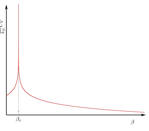
The specific heat CV, for Onsager’s exact solution near the critical temperature βc =√2 + 1 is
[40].
1
kBCV ≈
8β 2
c
π
·
−log
¯ ¯ ¯ ¯1−
β βc
¯ ¯ ¯ ¯+ log
¯ ¯ ¯ ¯
1 2βc
¯ ¯ ¯ ¯−
³
1 + π 4
´¸
(1.2.4)
A plot of Equation (1.2.4) is shown in Figure 1.1.
βc
1 kB
CV
[image:20.612.198.457.97.326.2]β
Figure 1.1: Specific heat of the two dimensional Ising model
1.2.2
Perturbation expansions
Perturbation expansion is a mathematical method used to approximate the solution of a problem
that cannot be solved exactly [50, 9]. In the absence of exact solutions to problems such as the
Potts model, we can find certain terms of the partition function and estimate certain expectation
values. For instance, Guttman and Enting [35] found a series for the free energy of theQ= 3-state
Potts model to around 40 terms.
Kramers and Wannier [51] used duality (discussed in detail in the next section) and perturbation
expansion to find the exact critical temperature of the 2d Ising model. Here we use their method
to explain perturbation expansions. We focus on the 2d square lattice, but the method can be
applied to any multi-dimensional lattice.
Recall, the partition function Z(T) (1.1.1), and the Ising model Hamiltonian H (1.2.1). Note,
with reference to Equation (1.2.1), we fixM = 0,ǫ= 1 and then expand the R.H.S..
Consider the model at low temperature K, on a 2d lattice withN sites. Suppose all spins are
pointing in the same direction. That is, either all up or all down (see Figure 1.2(a) for example).
Then, with periodic boundary conditions, we haveH =−2N, and the largest term in the series is
2e2N K (cf. Appendix C for further details).
Now if we flip any spin on the lattice (see Figure 1.2(b) for example), then four of the interactions
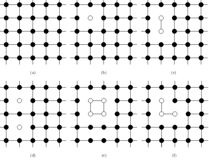
(a) (b) (c)
[image:21.612.115.539.12.345.2](d) (e) (f)
Figure 1.2: Showing the low temperature expansion for part of a 2d lattice. Full circles denote spins
pointing up, and open circles are spins pointing down.
up (or vice versa). Thus the next term is 2N e(2N−8)K.
The next term has 4N states when two adjacent spins are down and the rest are up (or vice
versa), see Figure 1.2(c). The change in the Hamiltonian from all up (or all down) is−12.
Figures 1.2(d)-(f), all have the same Hamiltonian value. This is a combination of: two
non-adjacent spins (Figure 1.2(d)); four non-adjacent spins forming a square (Figure 1.2(e)); or any three
adjacent spins (Figure 1.2(f)).
The partition function for the Kexpansion is
Z(K) = 2e2N K+ 2N e(2N−8)K+ 4N e(2N−12)K+N(N−5)e(2N−16)K+. . . (1.2.5) = 2e2N K(1 +N e−8K+ 2N e−12K+1
2N(N−5)e
−16K+. . .) (1.2.6)
= 2e2N KP(e−2K). (1.2.7)
whereP is a polynomial.
In a similar manner, we now consider the expansion at high temperature K∗. This time every
spin is pointing in the opposite direction to its nearest neighbours, see Figure 1.3(a). The leading
term in this case is 2e−2N K∗
. Then in a similar manner to the low temperature expansion, by
(a) (b) (c)
(d) (e) (f)
Figure 1.3: Showing the high temperature expansion for part of a 2d lattice. Full circles denote spins
pointing up, and open circles are spins pointing down.
The partition function for the K∗ expansion is
Z(K∗) = 2e−2N K∗(1 +N e8K∗ + 2N e12K∗ +12N(N−5)e16K∗ +. . .) (1.2.8) Note this series does not converge. However, we can write Z(K∗) in terms of tanh. That is, as
σiσj =±1, then we can use the identity
exp(βσiσj) = cosh(β) +σiσjsinh(β) = cosh(β)(1 +σiσjtanh(β)), (1.2.9)
to writeZ(K∗) as
Z(K∗) = 2Ncosh(K∗)2N(1 +Ntanh(K∗)4+ 2Ntanh(K∗)6+. . .) (1.2.10)
= 2Ncosh(K∗)2NP(tanh(K∗)). (1.2.11)
Note, the derivation of this expansion is explained in the next section (specifically, Equation
(1.2.24)). But for now, the graphical explanation of the low-temperature and high-temperature
expansions should make the correspondence between the two clear, ie. P(e−2K) = P(tanhK∗)
[50]. To justify this relationship, suppose we let
Then, we write Equation (1.2.7) as
Z(K) = 2 tanh(K∗)−NP(tanh(K∗)) (using (1.2.12))
= 2 tanh(K∗)−N£2−Ncosh(K∗)−2NZ(K∗)¤ (by Equation (1.2.11)) = 2 (2 sinh(K∗) cosh(K∗))−N
Z(K∗)
= 2 sinh(2K∗)−N Z(K∗) (1.2.13)
[1.7] Thefree energy density f (cf. [64]), is
f =−kBT lim N→∞
1
Nln(Z),
whereN is the number of spins. By Peierls argument (paragraph[1.6]) there exists a temperature
βc, whereK=K∗=βc and
−kBT lim N→∞
µ
1
N lnZ(K)
¶
=−kBT lim N→∞
µ
1
N lnZ(K
∗)
¶
+kTln(sinh(2βc)).
Thus, the critical temperature of the 2d Ising model is when
sinh(2βc) = 1,
thus
βc =
1 2ln(1 +
√ 2).
1.2.3
Duality
We can use duality to pass information we know about one model to its “dual” model (as we shall
see later). This is quite a powerful tool, as we show that certain properties of a model, that may
not manifest too easily on one may do so on its dual [9, 74]. For example, Figure 1.4 is a planar
representation of a triangular lattice and its dual honeycomb lattice. (See Baxter [9,§6,§12] for a
detailed example of this duality transformation.)
Duality transformations can be generalised to d-dimensional simple hypercubic lattices [36].
For example, Savit [86] shows that the 3d Ising model is dual to a lattice gauge model. See Martin
[60] for an example of this duality transformation.
Kramers and Wannier [51] showed that the 2d Ising model is self-dual. That is, the 2d Ising
model can be expressed as another 2d Ising model. They used duality to determine the critical
temperature for the 2d Ising model in a zero magnetic field (detailed in Section 1.2.2).
2d Ising model duality
Here we demonstrate how duality works for the 2dQ= 2 (Ising) Potts model. To begin, we recall
some graph notation [25]. Let G be a planar graph. We define a dual graph D(G), of a
plane-embedded graph G. We can then rewrite the partition function Z, on a lattice L, from Equation
(1.1.14) in a form that allows us to write a duality transformation between the partition functions
Figure 1.4: A section of a triangular lattice (black vertices and solid lines) and its dual honeycomb lattice
(white vertices and dashed lines).
Figure 1.5: A graphG (black vertices and solid lines) representing a 4×4 lattice, and its dual lattice
(white vertices and dashed lines).
Recall a graph G = G(VG, EG), with VG the set of vertices of G, EG the set of edges of G.
SupposeG is plane-embedded, and letFG be the set of faces ofG in this embedding. A face is a
region bounded by edges, and the set includes the outer infinite region. Note by Euler’s formula
that
|VG| − |EG|+|FG|= 2. (1.2.14)
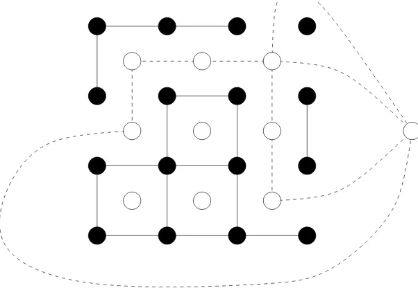
LetDbe the dual graph ofG (for example, see Figure 1.5). That is, in the centre of each face
ofG, we place a vertex ofD. And for each edge inG that separates two faces we draw an edge of
D, whose vertices are the vertices ofD that lie in the faces it separates. Also add a vertex ofD outsideG, that connect all edges on the boundary ofG. Note,GandDare not isomorphic to each
other in general, thus implying thatZD6=ZG. Also note
We now show how the partition function described in Equation (1.1.1) can be formulated in
terms ofGand its sub-graphs. LetG′be anedge sub-graphofG, writtenG′ ⊆ G. That is: V
G =VG′,
andEG′ ⊆EG.
Letx=eβ andv=x
−1, then
exp(βδσi,σj) = 1 +vδσi,σj (1.2.16)
so theQ-state Potts partition functionZG (Equation (1.1.14)), is rewritten as
ZG =
X
σ∈Ω
Y
<ij>∈EG
(1 +vδσi,σj), (1.2.17)
where < ij > represent the nearest neighbour interactions. Note each factor of the product
corresponds to an interaction (bond).
If we multiply out the product of Equation (1.2.17), then the terms of this expansion can be
represented by the edge sub-graphsG′
⊆ G. The edge sets ofG′ correspond to thevfactors in the
terms. After carrying out spin configuration summation, we can write the partition function in
the ‘dichromatic polynomial’ [97] form (see e.g. [8])
ZG =
X
G′⊆G
v|EG′|Q|CG′|, (1.2.18)
where|CG′|is the number of connected clusters inG′, including isolated vertices.
Now we fixQ= 2. Suppose we rewrite the factor exp(βδσi,σj) from the partition function, not
as in Equation (1.2.17) but as
(1 + (x−1)δσi,σj) =
µx+ 1
2 +
(x−1)
2 (2δσi,σj−1)
¶
. (1.2.19)
Then Equation (1.2.17) can be written as
ZG =
X
σ∈Ω
Y
<ij>∈EG
µ
x+ 1
2 +
(x−1)
2 (2δσi,σj−1)
¶
. (1.2.20)
By factoring out the largest term of the product we have
ZG=
µ
x+ 1 2
¶|EG|
X
σ∈Ω
Y
<ij>∈EG
µ
1 + (x−1)
x+ 1 (2δσi,σj −1)
¶
, (1.2.21)
=
µ
x+ 1 2
¶|EG|
X
σ∈Ω
X
G′⊂G
Y
<ij>∈EG′
µ
x−1
x+ 1
¶
(2δσi,σj −1), (1.2.22)
=
µ
x+ 1 2
¶|EG|
X
σ∈Ω
X
G′⊂G
µ
x−1
x+ 1
¶EG′ Y
<ij>∈EG′
(2δσi,σj−1). (1.2.23)
As an example consider the lattice consisting of a single square, andG′, a single edge. Here we
have
X
σ∈Ω
Y
<ij>∈EG′
(2δσi,σj −1) =
X
σ∈Ω
(2δσ1,σ2−1) =
X
σ∈Ω
2δσ1,σ2−
X
σ∈Ω
1
= 2X
σ∈Ω
δσ1,σ2−
X
σ∈Ω
Figure 1.6: An example of a mapping between graphG′
⊂ G (black vertices and solid lines) and a dual
ofG,D′
⊂ D(white vertices and dashed lines).
In fact, the sum is zero whenever the graph G′ describes a ‘non-even covering’ of
G. An even coveringis a sub-graphG′ such that every vertex has an even number of edges.
One sees that if G′ describes an even covering of
G, then the sum is always 2N. Thus we have:
ZG = 2N
µ
x+ 1 2
¶|EG|
X
even coveringsG′
µ
x−1
x+ 1
¶|EG′|
(1.2.24)
We now show a formulation of duality for the Q= 2 (Ising) Potts model in two dimensions.
LetDbe the dual graph ofG. Suppose for anyG′
⊆ G, we introduce an edge sub-graphD′
⊆ D such that ED′ is the complement set of EG′ (see Figure 1.6 for example). By construction the
connected components ofD′ form “islands” around clusters of
G′.
For theQ= 2 model, we can write the partition function explicitly in terms of the islands
ZD = 2xE
X
IslandsH
³
x−l(H)´, (1.2.25)
wherel(H) is the length of an island H andE=|ED|.
There is a bijection between the islands ofDand the coverings ofGthat takes sub-graphs onto
identical, but shifted sub-graphs.
Note that if G is self-dual, then the partition function is ‘almost’ invariant under the
transfor-mations [64]
x−1↔ x−1
x+ 1. (1.2.26)
(cf. (1.2.12) and (1.2.26).) Further, for theQ-state Potts model the duality relation is (see Martin
[62])
x→ x+ (Q−1)
The square lattice is almost self-dual, in the sense that in the square lattice is taken to another
square lattice up to boundary effects. (cf. Figure 1.5 with the self-dual lattice in Chen et al. (1996)
[19], Figure 1).
The invariance property of the model is then called self-duality. In this sense, self-duality for
the square lattice model holds true ‘up to boundary effects’.
[1.8] More generally, and more precisely, letP be a polynomial in 1
x, such that Equation (1.2.25)
is written as
ZD= 2xEP
µ
1
x
¶
(1.2.28)
Then
2N
µ
x+ 1 2
¶E
P
µ
x−1
x+ 1
¶
=ZG. (1.2.29)
(Compare with Equation (1.2.13)).
Example 1.1. FixQ= 2, usingG andDfrom Figure 1.5, then by Equation(1.2.24)we have
ZG = 2 + 8x2+ 32x3+ 72x4+ 224x5+ 584x6+ 1216x7+ 2638x8+ 4928x9+
+ 7344x10+ 9984x11+ 11472x12+ 9984x13+ 7344x14+ 4928x15+
+ 2638x16+ 1216x17+ 584x18+ 224x19+ 72x20+ 32x21+ 8x22+ 2x24, (1.2.30) and by Equation(1.2.25)
ZD = 2x4+ 8x6+ 138x8+ 232x10+ 316x12+ 184x14+ 100x16+ 24x18+ 18x20+ 2x24. (1.2.31)
The zeros of Equations(1.2.30)and(1.2.31)are plotted in Figures 1.7(a) and 1.7(b) respectively.
The zeros are invariant in the dashed grey circle shown. Plotting the zeros in the same plane (Figure
1.7(c)), highlights the invariance property. Figure 1.7(d), displays the distribution of zeros forP(x−1)+
P(x+1
x−1).
We shall use this duality relation to validate our results in Chapter 3, and discuss the importance
of the dashed grey circle.
1.2.4
Monte-Carlo methods
One of the most popular methods used in approximating observables is using aMonte-Carlo method
[52]. There are quite a few different types of Monte-Carlo algorithms, but the overall concept is
the same. Here we describe a Monte-Carlo algorithm known as the Metropolis algorithm [72]. We
shall discuss some of the advantages and disadvantages of Monte-Carlo methods.
In general, the Metropolis algorithm uses a manageable sized sample of configurations. From
this sample, we can approximate observable data. The algorithm works by considering suitable
changes in energyδE between states. The algorithm is as follows [52]:
1. Choose an initial state.
(a) Zeros ofZGfrom Equation (1.2.30). (b) Zeros ofZDfrom Equation (1.2.31).
(c) Overlay of Figures (a) and (b). (d) Zeros of the sum of P from
Equa-tion (1.2.28) and (1.2.29)
Figure 1.7: Various zeros of a 2d Potts model withQ= 2 fixed on graphsGandDfrom Figure 1.5. The solid cross represents the unit axis of the complex temperature plane.
3. Calculate the change in energyδE, if the spin at siteiis changed/flipped.
4. Generate a random numberr, in the interval [0,1].
5. Ifr <exp(−δE/kBT), change/flip the spin.
6. Iterate from step 2.
Thermal averages from this sample can then be calculated.
An estimate of the critical pointβcfor the 3d Ising model, on a simple cubic lattice (by Talapov
and Bl¨ote (1996) [92]) is
βc=J/kBTc= 0.2216544, (1.2.32)
with a claimed standard deviation of 3×10⁻⁷. A Monte-Carlo algorithm was used to compute
this result. It was checked against the exact solution of the 2d Ising model.
The advantages of using the Monte-Carlo method, lie within the advantages of sampling
tech-niques. When analytic techniques fail, the Monte-Carlo method can be used to give an insight
into the behaviour of the system. Due to the limitations of computer speed and memory, for large
systems with an extremely large number of configurations, approximating may be the only way to
How true or fair are all possible configurations being represented by our sample of
configura-tions? The results obtained using Monte-Carlo methods are exposed to statistical error. That is
because we are looking at a sample of the population (ie. all possible states/configurations of the
system). However, the accuracy of the system (reducing the magnitude of the statistical errors)
may be increased simply by increasing the sample size (including more states). This does require
further processor time. Also questions arise on how many computations are carried out for the
sample to be accurate and in thermodynamic equilibrium (for example, how many iterations should
we carry out; what the size of the sample should be; etc...).
1.2.5
Existing exact finite lattice results
In this section, we discuss some publishedQ-state Potts model results on finite 2d and 3d lattices.
In 1982, Pearson [81], found the exact partition function for the 3d Ising model on 4×4×4
simple cubic lattice. He obtained his result by identifying symmetries that significantly reduced
the number of configurations to be enumerated from 264 to 232.
In 1990, Bhanot and Sastry [10] calculated the partition function for a 4×5×5 lattice. To
compute this result they used the Connection Machine, a “massively” parallel computer. Using
the Connection machine, they were able to enumerate the states of the partition function using
220processors.
For the Q >2 state Potts model on 2d and 3d lattice see Martin [61, 66, 63, 64]. Martin has
used a transfer matrix approach (§2.2.1) to obtain his results . In his paper we also find some
interesting anisotropic [64] 2d Potts model results, such as the 5 and 6-state models on a 6×7
lattice.
1.3
Physical interpretation of results
Our focus of study is on phase transitions, and what happens to a material as the critical
temper-ature is approached. Phase transitions manifest as singularities in our results [64, §1.4.2]. Phase
transitions are classified by where the lowest derivative of the free energy is discontinuous (cf.
[39]). For example, we say it is a first order phase transition if the first derivative is discontinuous.
Divergence in the specific heat (§1.1.3) is a signal of a second-order phase transition.
In statistical mechanics, we use correlation functions to measure how spins at various points
on the lattice interact. In our systems, correlation functions contain important information about
physical phase transitions [40]. Close to the critical temperature thespin-spin correlation length
diverges [50,§II.A], and this can be interpreted as a signal for a second-order phase transition.
The zeros of the partition function are a powerful tool used for studying phase transitions and
critical phenomena in finite-size systems [32]. In 1965 Fisher [30] considered the Ising model as
a polynomial (in the variablee2β), and studied the behaviour of its zero distribution. He showed
that, in the thermodynamic limit (cf. Blundell [13, §1.2]), phase transitions occur where the
such stabilising features that may occur can be interpreted as an indication of what may happen
in the thermodynamic limit.
1.4
Universality
Recall, a critical point of a system is a time-independent property of where phase transition occur.
It separates the system into phases. Order parameters [49, 64] describe the phase a system is in.
The average magnetisation of a ferromagnet and the density of a liquid-gas material are examples
of order parameters [69]. Critical exponents describe the behaviour of order parameters near a
transition2.
According to theuniversality hypothesis, the critical behaviour of a system depends on
prop-erties such as the dimension of space and the symmetries of the system [9, 34, 69]. That is
“If we could solve a model with the same dimensionality and symmetry as a real
sys-tem, universality asserts that we should obtain the exact critical components of the real
system.” – Baxter (1982) [9].
Each system is assigned to a universality class [52]. Systems that have the same set of critical
exponents belong to the same universality class. For example, universality puts a liquid-gas
tran-sition and Ising magnet trantran-sition into the same class [69,§8.1.3]. Also according to universality
the gas-liquid phase transition of carbon dioxide, the gas-solid phase transition of xenon and the
phase transition of the 3d Ising model should be in the same class [9].
In the following chapter, we present a method for finding the critical temperature of the 3d
Ising model. First we describe a method to compute partition functions for the Q-state Potts
model, and then study the specific heat order parameter. We present our results in the form of
zeros distributions and specific heat plots in Chapter 3.
2
Chapter 2
Computational Method
For Potts models on lattices of any significant size, to calculate the partition function by a
brute-force enumeration of states is not feasible. For this reason, technical tools such astransfer matrices
are now introduced [9,§7.2].
In order to introduce transfer matrix formalism we start by recalling the necessary mathematical
machinery and notations in a slightly more general setting. We have in part followed the analysis
by Martin (1991) [64] in this chapter.
2.1
Potts models on graphs
Basic notations for spin configurations
ForQa natural number, define the setQ={1,2, . . . Q}. For us, then,Q-state Potts spin variables
can be considered to take values fromQ.
ForS, T sets we write hom(S, T) for the set of all maps fromS toT [45,§1.6].
If a set S indexes the spins in a given Potts model (for example, the set of physical locations
might serve this purpose) we shall write ΣS for the set of spins.
The set of all spin configurations of some set ΣS ofQ-state Potts spins is thus
ΩS := hom(ΣS, Q)
Note that mathematically this is the same as hom(S, Q).
LetAbe some finite set of symbols [28]. A string overAis a finite sequence of symbols drawn
from that set. LetAk denote the set of all strings over Aof lengthk.
Example 2.1. FixQ= 2, thenQ3={111,211,121,221,112,212,122,222}.
Apply a total order Ron set S, and writeσi for theith spin in this order. We can then write
ΩS as a set of strings. That is, for eachf ∈ΩS we may encode it as an element of Q|ΣS|by
f(σi) =xi (2.1.1)
G
c a
b
Figure 2.1: A planar realisation of an undirected graphG.
Similarly we can think of each f ∈ΩS as a|ΣS|-tuple vector: theith element of f isf(σi).
Example 2.2. For Q= 2 fixed, we have the set Q3. Let S ={1, a,3}. Assume that a total order relationR, orders the elements ofS as a <1 <3. Also let ΣS ={σ1, σa, σ3}. Then for 712∈Q3,
the corresponding functionf ∈ΩS is
f(σ1) = 1, f(σa) = 7 and f(σ3) = 2. (2.1.2)
This is also written as vector(f(σa), f(σ1), f(σ3)), which evaluates to(7,1,2).
Graphs as Potts model ‘lattices’
Recall [25,§1.1] that a simple undirected graphG=G(VG, EG) is a set of verticesVGtogether with
a set of edgesEG, which are unordered pairs fromVG.
Example 2.3. Figure 2.1 encodes a graphG, with three arbitrarily labelled verticesa,b andc. That is
VG={a, b, c},EG ={{a, b},{a, c},{b, c}}.
A lattice spin system [50] is modelled here as a Potts model on a simple undirected graph
G(VG, EG) [101]. A vertexi∈VG represents a physical site on the lattice, on which resides a spin
σi; and the set of edgesEG represents the bond or nearest neighbour interactions between spins.
For each choice of graph G and natural number Q we have the Potts model Hamiltonian (cf.
Section 1.1.4):
HG: ΩVG →R
HG(f) =
X
{i,j}∈EG
δf(σi),f(σj). (2.1.3)
Where δa,b is theKronecker delta, that returns a value of 1 if a=b, and 0 otherwise. We shall
writeHG as justH, when the dependence onGis clear.
Example 2.4. UsingG from Example 2.3 withVG totally ordered in the natural way and configuration
(1,2,2)∈ΩVG, the Hamiltonian value is
G
c a
b
V
Figure 2.2: Shows setV ⊆VG.
The notion of Potts partition function Z [40] can then be regarded as a map from the set of
graphsG to the set of polynomials ZG in exp(β). That is (cf. Equation (1.1.1)):
ZG =
X
σ∈ΩVG
expβHG(σ). (2.1.5)
Here physicallyβ =−1/kBT (kB is Boltzmann’s constant,T the temperature). For the remainder
of this section letx= exp(β).
Example 2.5. Using Gfrom Example 2.3, and fixing Q= 2, thenZG= 2e3β+ 6eβ.
2.2
Partition vectors and transfer matrices
In this section. Partition vectors [64,§2.1] will be explained. A specialisation to transfer matrix
formulation is then made in Section 2.2.1.
Let V ⊆VG for any graphG. ForQ-state Potts model configuration c∈ΩV, we define ΩVVG|c
as the set of spin configurations where the spins associated toV are fixed toc. Note ΩV
VG|c⊂ΩVG.
Example 2.6. LetVG ={a, b, c} andV ={a, c} (see Figure 2.2). FixQ= 2. Take the natural order
onVG, and the natural order by restriction of this order onV, then
ΩVG ={(1,1,1),(2,1,1),(1,2,1),(2,2,1),(1,1,2),(2,1,2),(1,2,2),(2,2,2)}, (2.2.1)
andΩV ={(1,1),(2,1),(1,2),(2,2)}. Then for configuration (1,1)∈ΩV, we have
ΩVVG|(1,1)={(1,1,1),(1,2,1)}. (2.2.2)
The partition function with the configuration of spins in subset V fixed to configuration c
(c∈ΩV) is
ZGV|c:=
X
σ∈ΩV VG|c
exp(βH(σ)). (2.2.3)
Definition 2.2.1. The partition vectorZV
G is a vector indexed byΩV.
Thec-th component ofZV
G (c∈ΩV) isZGV|c. Note
ZG =
X
c∈ΩV
Example 2.7. Consider graph G in Figure 2.2, where the subset of vertices V ={a, c} is indicated.
FixQ= 2. We haveΣV ={σa, σc}, and
ZGV =
¡
ZGV|(1,1), ZGV|(1,2), ZGV|(2,1), ZGV|(2,2)
¢
(2.2.5)
=¡x3+x, 2x, 2x, x3+x¢. (2.2.6)
Note, summing up the entries ofZV
G giveZG from Example 2.5.
[2.1] We now formulate a method for combining the partition vectors for two Potts models on graphs to make a Potts model partition function for a larger graph. We refer to this asbinding.
To do this, first we must define the union operator of two graphs (cf. [94] for several variations on
combining graphs).
Definition 2.2.2. For the unionG ∪ G′ of graphsG andG′, we have:
VG∪G′ =VG∪VG′ and EG∪G′ =EG∪EG′.
Theorem 2.2.3 (Chapman-Kolmogorov [80]). Let G and G′ be graphs such that E
G∩EG′ =∅.
Let GG′ denote
G ∪ G′ andV =V
G∩VG′. Then
ZGG′ =
X
c∈ΩV
(ZGV|c)(ZGV′|c) =ZGV ·ZGV′ (2.2.7)
Proof. Recall Equation (2.1.5). For graphGG′ =G ∪ G′, we have
ZGG′ =
X
σ∈ΩVGG′
eβHGG′(σ) (2.2.8)
ProvidingEG∩EG′ =∅, then
HGG′(σ) =HG(σ) +HG′(σ). (2.2.9)
for every configurationσ∈ΩVGG′. Thus
ZGG′ =
X
σ∈ΩV
GG′
³
eβHG(σ)´ ³eβHG′(σ)
´
(2.2.10)
Now ifV =VG∩VG′ then
ZGG′=
X
c∈ΩV
X
σ∈ΩVG |c
eβHG(σ)
X
σ′∈ΩV G′|c
eβHG′(σ′)
(2.2.11)
= X
c∈ΩV
¡
ZGV|c¢ ¡ZGV′|c¢ (2.2.12)
The second identity in Equation (2.2.7) is an equivalent statement by Definition 2.2.1.
Example 2.8. FixQ= 2. For graphsG andG′, see Figure 2.3. The partition vectorZV
G is
(ZGV|(1), ZGV|(2)) = (x3+ 3x, x3+ 3x). (2.2.13)
Also
c a
b
G
V
V c
G′
a′
b′
Figure 2.3: GraphsG andG′
c a
b
V
a′
b′
GG′
Figure 2.4: The resultant graphGG′
, obtained by combiningG andG′
(from Figure 2.3) overV.
Then for graphGG′=G ∪ G′ (Figure 2.4),V
GG′ ={a, a′, b, b′, c},V ={c}, and
ZGG′ =¡ZGV|1·ZGV′|1
¢
+¡ZGV|2·ZGV′|2
¢
= (x3+ 3x)(x2+ 2x+ 1) + (x3+ 3x)(x2+ 2x+ 1)
= 2x5+ 4x4+ 8x3+ 12x2+ 6x (2.2.15)
A mild generalisation of Theorem 2.2.3 is as follows.
Notation: For setsV andV′ letV
\V′ denote the set of all elements inV that are not inV′.
Lemma 2.2.4. LetGandG′ be graphs such thatE
G∩EG′ =∅. LetGG′=G ∪G′ andV =VG∩VG′
andV′
⊆VGG′. Then
ZGGV′′|c′ =
X
c∈ΩV\V′
(ZGV|c′c)(ZGV′|c′c). (2.2.16)
Here c′c is the configuration associated to V′ and then toV.
The proof of Lemma 2.2.4 is similar to the proof of Theorem 2.2.3 (cf. Chapman-kolmogorov
G G′ GG′
V V
VG′∩V′
V′
VG∩V′
I E
Figure 2.6: Representing incoming and outgoing spins usingI andE respectively
equation [80]). Figure 2.5 is a graphical representation of Lemma 2.2.4. The next section shows
how Lemma 2.2.4 implies matrix multiplication can be used to combine partition vectors.
2.2.1
Transfer matrices
In this section we show that the partition function (Equation (2.1.5)) is for certain very regular
graphs Gthe trace of the Nth power of a certain matrix. We call this matrix thetransfer matrix
[88, 12, 9, 6, 65, 85, 23]. A computational feature of using transfer matrices is that we may compute
ZG by repeatedly binding smaller systems together.
Recall the partition vector ZV
G. LetE ⊂V. We call ΣE the set ofoutgoing spins. LetI ⊂V
such that V = E ∪ I. Call ΣI the set ofincoming spins. ZGV is now trivially reorganised as a
matrix, denoted T. The rows and columns of T are indexed by ΩI and ΩE respectively. The
element in thei-th row,j-th column is
Tij =ZGI,E|i,j, (2.2.17)
where i ∈ ΩI and j ∈ ΩE. Indeed for any collection of subsets Vi ⊂ V such that V =∪iVi we
define ZV1,V2,...
G |c1,c2,... in the obvious way — leading to what might be called apartition tensor
[64, 46].
Example 2.9. FixQ= 2. Let the graph in Figure 2.6 model a spin system. The incoming and outgoing
vertex (spin) sets have been labelledI andE respectively. Then
T =
x3 x x x
x2 x2 1 x2
x2 1 x2 x2
x x x x3
(2.2.18)
LetTGandTG′ be transfer matrices associated to graphsGandG′respectively, withIG,EG and IG′ andEG′ being the index sets to the incoming and outgoing spins for TG andTG′ respectively.
IfEG =IG′, andEG∩EG′ =∅ then by Lemma 2.2.4, we have the matrix product
TGG′ =TGTG′. (2.2.19)
G G′ GG′
Figure 2.7: Spin systems modelled by graphsG andG′
andGG′
, whereG andG′
are connected to form
GG′
. The red, white, and black vertices model incoming, outgoing, and internal spins respectively.
After matrix multiplication, any further binding with TGG′ is restricted to incoming and
out-going spins of GG′. The set E
G∩ IG′ becomes the set ofinternal vertices of GG′. That is, the
spin configuration information of these vertices is summed over, such that no further binding from
these vertices is possible. We shall often refer to these spins as internal spins.
For an example of such graphs see Figure 2.7. Here we model incoming, outgoing, and internal
spins in each graph using red, white and black vertices respectively.
The partition function for a suitable large regular graph (such as a crystal structure cf. §2.2.2)
can then be calculated by iteratively multiplying suitably smaller manageable transfer matrices.
To do this, we introduceisomorphisms between graphs.
Definition 2.2.5. Two graphs G and G′ are said to be isomorphic [18] if there is a one-to-one
mappingφ:VG →VG′ such that if and only if{a, b} ∈EG then{φ(a), φ(b)} ∈EG′.
For instance, supposeGis isomorphic (in the strong sense) toG′, and|E
G|=|IG|=|EG′|=|IG′|
then we can takeTG =TG′. It then follows that
TGG′ =TGTG′ = (TG)2. (2.2.20)
LetG(L) be the graph union ofL isomorphic graphsG. The partition function is given by
ZG(L)=
X
s∈ΩIG(L)
X
t∈ΩEG(L)
¡
TGL|st
¢
(2.2.21)
where IG(L) is the incoming spin set for G(L) (ie. IG for the first G in G(L)); and EG(L) is the
outgoing spin set forG(L) (ie. EG for the lastGinG(L)). Note that ifDis the column vector with
Di= 1 for all configurations in ΩIG then
ZG(L)=DTTLD. (2.2.22)
To obtain periodic boundary condition (Section 2.2.2) we identify the incoming and outgoing spins
of (TG)L. To do this, we sum over the states where incoming and outgoing configurations are equal.
Specifically
2.2.2
Geometry and Crystal lattices
This section is on graphs as regular crystal lattices [71] embedded in Euclidean space [31, 36].
Potts Model in d-dimension
We ‘place’ spins inRdso as to form ad-dimensionallatticemodelling a physical crystal lattice. Let
Ld denote thed-dimensional hypercubic lattice. Here, we define
L=Ld as a finite set of regularly
spaced sites embedded in the Euclidean spaceRd of the form {{1, . . . , N1} × {1, . . . , N2} ×. . .×
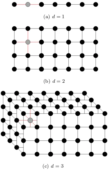
{1, . . . , Nd}|Ni ∈N}. On each site resides a spin. Figure 2.8, the sub-figures depict examples of
d-dimensional lattices. We draw lines between nearest-neighbour sites to represent corresponding
interactions between spins.
(a) d= 1
(b)d= 2
[image:38.612.240.412.197.473.2](c)d= 3
Figure 2.8: Showingd-dimensional lattices. The grey spin in each figure, represents a typical bulk spin and its nearest neighbour interactions (red edges).
Layer transfer matrix
Our d-dimensional lattice can be built up by a set of (d−1)-dimensional sub-lattices. We shall
call theselayers of a lattice. Note, in the case ofd= 1, a layer is just a single point.
In d= 3 we shall use the notation Nx×Ny×Nz, (Nx, Ny, Nz ∈N) to represent L with Nz
layers. Each layer hasNycolumns each containingNxsites. The total number of sites isNxNyNz.
For the Q-state Potts model on L, the ith layer interacts only with the i−1th andi+ 1th
layers.
Now suppose we wanted to calculate a Q-state Potts model partition function on a lattice
d= 3
d= 2
d= 1
Figure 2.9: Examples of d-dimensional transfer matrix lattice layers. Incoming (outgoing) spins are modelled by grey (white) vertices
layers. We shall refer to this as the “layer transfer matrix”. NoteT is aQNxNy×QNxNy matrix.
Figure 2.9 are examplesd-dimensional transfer matrix lattice layers.
For the remainder of this Thesis we shall only be concerned with the given regular crystal lattice
structure, and graphG(Section 2.1) shall be regarded as a lattice in the obvious way. Further, we
shall refer to the partition function as justZ.
As we have seen, where it can be applied, the transfer matrix formalism speeds up partition
function calculations. If in addition, as in crystal lattices, the layer has symmetry, then some
further speed-ups can be achieved. In Appendix B, we show how to use such symmetries ofT to
findTL for relatively large
T.
Boundary Conditions
In dimensiond, the numbernof nearest neighbours to each spin isn= 2dup to boundary effects
[21]. A finite-sized lattice (as defined so far) has spins on the boundary of the lattice that have
n <2d. We refer to this as the lattice having open boundary conditions. The lattices in Figure
2.8, are examples of lattices with open boundary conditions.
An alternative is to introduce an extra interaction between spins on opposite sides of the
boundary. In this case all spins on a lattice have the same number of nearest neighbours, and
there are exact translation symmetries. We refer to this as applyingperiodicboundary conditions.
2.2.3
Eigenvalues of the transfer matrix
Recall the layer transfer matrixT, Section 2.2.1, such as in Example 2.9.
For thisT, all entries are monomials inx=eβ. In particular all entries are positive for realβ.
SupposeT binds layersiand i+ 1. Then by Theorem 2.2.3, we may write T as a product of
morelocal transfer matrices, sayTi+1,Ti,i+1. SpecificallyTi+1is restricted to only the interactions
Example 2.10. ForT in given in Example 2.9 (page 23)
T =Ti,i+1Ti+1=
x2 x x 1
x x2 1 x x 1 x2 x
1 x x x2
x 1 1 x
[2.2] By symmetry of the Hamiltonian, Ti,i+1 and Ti+1 are Hermitian matrices for realβ. Note,
they both are real symmetric andTi+1 is also a diagonal matrix. One can then show that T is
similar (in the technical sense) to a real symmetric matrix (and hence Hermitian).
Let {λi} be the set of eigenvalues ofT. Also, for each λi, let v′i and vi be the corresponding
row and column eigenvectors respectively. That is
Tvi=λivi (2.2.24)
and
vi′T =λiv′i. (2.2.25)
For us let r andw be suitable boundary vectors (such as DT and
Dfrom Equation (2.2.22)) such that
Z=rTNw.
Define coefficientsai andbi by
r=X
i
aiv′i and w=
X
i
bivi (2.2.26)
Note thatai andbi are constants, depending only on the fixed boundary conditionsrandw.
Then
rTN w=
à X
i
aiv′i
! TN X j
bjvj
(2.2.27) = Ã X i ai ¡
λNi vi′
¢ !
X
j
bjvj
(2.2.28)
By the similarity of T to a real symmetric matrix, eigenvectorsv′
i andvj can be chosen to be
orthonormal. Thus, bycompleteness of the set of eigenvectors [73], we have
λNi v′ivj=
λN
i , j=i
0, otherwise , (2.2.29)
for alli, j.
Thus Equation (2.2.28) simplifies to
rTN w=X
i
(aibiλNi ) (2.2.30)
so
Z=rTN w=X i
KiλNi , (2.2.31)