Rochester Institute of Technology
RIT Scholar Works
Theses Thesis/Dissertation Collections
2010
A PCA based method for image and video pose
sequencing
James Massaro
Follow this and additional works at:http://scholarworks.rit.edu/theses
This Thesis is brought to you for free and open access by the Thesis/Dissertation Collections at RIT Scholar Works. It has been accepted for inclusion in Theses by an authorized administrator of RIT Scholar Works. For more information, please [email protected].
Recommended Citation
A PCA Based Method for Image and Video Pose Sequencing
by
James Massaro
A Thesis Submitted
in
Partial Fulfillment
of the
Requirements for the Degree of MASTER OF SCIENCE
in
Electrical Engineering
Approved By:
PROF.
Thesis Advisor- Dr. Raghuveer Rao
PROF.
Thesis Committee Member- Dr. Sohail Dianat
PROF.
Thesis Committee Member- Dr. Ferat Sahin
PROF.
Electrical Engineering Department Head- Dr. Sohail Dianat
DEPARTMENT OF ELECTRICAL AND MICROELECTRICAL ENGINEERING
COLLEGE OF ENGINEERING
ROCHESTER INSTITUTE OF TECHNOLOGY
ROCHESTER, NEW YORK
THESIS RELEASE PERMISSION
ROCHESTER INSTITUTE OF TECHNOLOGY
DEPARTMENT OF ELECTRICAL AND MICROELECTRICAL ENGINEERING
Title of Thesis:
A PCA Based Method for Image and Video Pose Sequencing
I, James Massaro, hereby grant permission to Wallace Memorial Library of R.I.T. to
reproduce my thesis in whole or in part. Any reproduction will not be for commercial use
or profit.
Signature
Date
Dedication
I would like to dedicate this thesis to my fianc´e Stephanie and my parents because of all
Acknowledgments
First, I would like to thank my advisor, Dr. Raguhveer Rao for his instruction and
assistance. I would also like to thank my committee members Dr. Ferat Sahin and the
Department Head, Dr. Sohail Dianat for finding time to listen and make recommendations
for a better thesis. A special thanks to Dr. Ferat Sahin for encouraging me to do my best
with writing to make this thesis something I will be proud of for the rest of my career and
Abstract
Problems exist in image sequence processing that require an ordered set of object views.
In some cases, multiple angled images are acquired in random order and the angle of view
information is not available. When this occurs, the poses have to be put into proper order.
For example, in databases containing images of an object or scene taken over a period of
time, each image pose or angled-view with respect to the camera or scene is unknown.
This is important to achieve a complete or partial three-dimensional reconstruction. Other
applications exist in photogrammetry, machine vision, computer-aided design, and
mili-tary intelligence. The main contribution of this thesis is an automated method for ordering
images of random object views. This method uses Principal Component Analysis (PCA)
and a confidence metric in eigenspace. The confidence measure is based on local
curva-ture and correlation of the estimated pose trajectory in a multidimensional manifold. The
use of the confidence metric is for detecting areas in the manifold where poses appear
similar and ordering becomes difficult. It has been extended for use with synchronized
double and multiple camera system by providing a basis for camera selection, choosing
the most salient camera view for pose ordering. By adding multiple cameras, a high
pose estimation accuracy can be achieved. This thesis compares other classification and
recognition methods such as the Scale Invariant Feature Transform (SIFT) and Laplacian
Eigenmaps. The SIFT algorithm struggles with pose sequencing because it computes
lo-cal feature spaces for each image and does not consider the entire set of images. Laplacian
eigenmaps show better results for ordering, but close analysis show it is better suited for
clustering poses than sequencing. Results for ordering many set of objects, theoretical
Chapter 1
Introduction
1.1
Overview
Digital image processing (DIP) is a field that utilizes mathematical theories and models
with various applications. DIP is a broad term that includes several more specific areas of
research. A few areas of research in DIP include but are not limited to pattern recognition,
computer vision,artificial intelligence, surveillance, automation, and 3D modeling. These
areas of research utilize motion estimation, and image segmentation to perform a
recog-nition task. For example, law enforcement uses facial recogrecog-nition software to identify
criminals [1].
The ultimate goal for most advanced DIP systems is to control machines to perform
a specific task or to notify the user of a specific event. Recognition tasks notify the user
when a specific object has been identified. One problem inherent to performing these
tasks is recognition at varying pose or view-angle. An object that is not perfectly aligned
shape and illumination differences. One proposed solution for solving this problem is
to construct a training database that encompasses the entire 360◦ rotation of the object.
However, a continuous sampling of an objects rotation cannot be achieved. This is called
pose resolution, and it leads to another possible source of error. To fix this problem, a
method for pose recognition must be developed.
The most common way to perform pose recognition is by constructing a database of
angled-views. This can be done in two ways, either by manually taking images or videos
of an object in a laboratory, or through an unsupervised method of actively acquiring data
through a strategically placed camera(s). The unsupervised method has two drawbacks:
1. It is difficult and time consuming to place labels on the information that is being
acquired, and
2. the pose database is unordered and needs to be reordered to verify that there is
enough data for proper pose recognition. The amount of data needed for object
pose recognition is determined by its pose resolution.
Other supervised methods capable of recognizing an object in a scene at different
scales and poses have been developed by [2, 3]. These types of algorithms can recognize
the object up to certain pose angle until features become occluded or unrecognizable from
illumination changes.
This thesis proposes an unsupervised object pose ordering algorithm seen briefly in
the research by Massaroet al.[4]. It uses a confidence metric to find possible pose errors
because of indistinguishing views. This method is extended to a multiple camera
frame-work for improved sequencing. The proposed method could also be used in other
These topics will be discussed in more detail within the following chapter.
1.2
Random Object Poses
This section discusses the definition of an ordered set of object poses and an unordered
set of random object poses. Proceeding this is the motivation for pose ordering. This
includes database sequencing and 3D model construction, unsupervised learning for facial
databases, and path planning for unmanned aerial vehicles (UAVs). These are all possible
applications for ordered sets of object poses seen as an improvement to current algorithms.
1.2.1
What are random object poses?
Figure 1.1: Example of a video sequence (top) and a randomized video sequence
(bot-tom).
The pose of an object is the view-angle at which an object is observed. Each angled-view
or pose induces illumination changes and 2D shape variation creating different observable
poses. Monotonically changing angled-views of an object can be captured by a by a
stationary video camera and a turntable. The motion video captures an ordered set of
object poses. Contrarily, an unordered set of object poses are non-monotonically changing
angled-views of an object. The non-monotonicity of the view-angle is a random set of
object poses. This can be seen in Figure 1.1 where the top figure is an ordered set of
poses, and the bottom sequence is a random set of poses.
1.2.2
Image Databases
The initial motivation for pose ordering was to create a way to automatically find stereo
matching images in a series of random, unordered images. Stereo matching pairs can be
used to create a rough 3D model of the scene or object. The disorderedness of image
poses in the same scene occurs when images are taken at different times under varying
perspective. These types of images are required for capturing perspectives of a scene for
constructing a 3D model.
Random views of objects or scenes can be found in many real-world applications.
Some of these situations are found in remote sensing, and aerial surveillance. The
sit-uation of randomness occurs frequently in these sitsit-uations because of the variability in
viewing angle of air-born vehicles. The need for an alternative image-perspective based
algorithm arises because GPS and geo-referencing is not enough or may not have been
available to reorder images. The research by O’Dwyer et al. [5] use old imagery from
1953-1972 when the technology was not available for image geo-referencing.
Further-more, these types of images are taken over a period of time under varying circumstances
for the type of mission. For this reason, the perspectives of the same area result in different
Further research has indicated the necessity of ordered images for
photogrammet-ric methods [6]. It has been stated in this research that automated ordering of random
image databases would reduce the effort of ordering manually, which is costly and time
consuming. Moreover, this research states that these processes struggle with making
mea-surements from images with unordered data sets.
1.2.3
Machine Learning
Another motivation for object pose ordering is for supervised pose recognition of objects.
These methods refer to the design of a training databases from random views of an object.
The research in [7] outlines a system for the unsupervised acquisition of human faces for
a humanoid robot. The method explains that this can be achieved when objects and faces
are presented randomly to a camera. Each object or face is grouped into a pose database.
The database requires a method for unsupervised ordering to develop accurate training
data. Human interaction is optional for acquiring labels to faces. The human interaction
is involved in this method is known as inductive learning, while the faces are acquired and
ordered in an unsupervised fashion. Chapter 2 discusses how knowledge of the relative
1.3
Thesis Organization
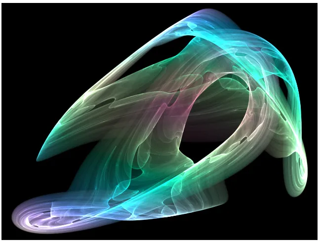
Figure 1.2: A visual example of a manifold. This image was obtained under the GNU
Free Document License
The following chapters will explain the research path for object pose ordering. Chapter 2
discusses the previous work conducted that relates to this thesis. This includes 3D model
construction methods, image matching, object recognition, image manifolds, and object
pose recognition methods. An example of a manifold can be seen in Figure 1.2. The
research in this section leads to the development of the methodology that will be used
for object pose ordering. Chapter 2 introduces the problem of pose ordering in terms
of Principal Component Analysis (PCA) space. Furthermore, this chapter describes the
detailed explanation of the method, including mathematical derivations and explanations
of hardware configuration and metrics used for object pose ordering. Chapter 4 contains
results obtained for single and two camera pose ordering, as well as results for a pose
clustering method. Chapter 5 contains the summary, possible future work and testing for
Chapter 2
Related Research and Problem
Formulation
This chapter focuses on research relating to computer vision and pose estimation problems
with emphasis on research related to pose ordering or image sequencing. This includes
image matching, object and face pose recognition, and object manifold analysis.
Fur-thermore, methods that combine pose information from 2D images for constructing 3D
image models is of interest in this section. Researching the relation between combining
2D information for stereo matching and computer recognition was a priority. It is thought
that the ability to link these methods is required for pose sequencing tasks because most
2.1
3D Image Reconstruction and Modeling
The purpose of this section is to document some of the methods used in 3D model
re-construction from 2D images. The methods for 3D object rere-construction from 2D images
requires knowledge of the object’s pose relative to the camera. Examples of reconstruction
algorithms can be found in [8–10]. The methods have trouble matching object geometry
with motion, unless a prioriknowledge of the sequence of poses is available. This
indi-cates reordering the image sequence to monotonically changing angled views is necessary
for accurate 3D reconstruction.
2.1.1
Structure and Motion Estimation
Joshi et al. [11] describe a method that recovers the shape of an object using three
cal-ibrated cameras. Epipolar geometry is used to find matching frontier points between
cameras in an attempt to recover the structure of the object. The motion can be predicted
and tracked from the silhouette profiles once the structure is known. This method is useful
when the object has very little or no surface features to distinguish between perspective
views. The method would not work well for pose sequencing and struggles with objects
that have similar silhouette shapes. Moreover, using motion estimation to order object
poses is impossible when then the image sequence is random.
2.2
Scale Invariant Feature Transform
The scale-invariant feature transform (SIFT) will be the described in this section. SIFT
image mosaicking [12]. In [13], Brown et al. describe a method using SIFT to find
point correspondences between multiple cameras using epipolar geometry. The
corre-sponding points between images were run through a random sample consensus algorithm
(RANSAC) to eliminate outliers. The maximum number of corresponding points
be-tween images represents an image match. A sparse 3D model is constructed from the
point correspondences using epipolar geometry. This is just one example of a method that
has appeared using SIFT. Other research includes [14] which uses PCA as a local image
descriptor.
The first research was presented by Lowe [15] and has been referenced by many and
has been the foundation for many other image matching algorithms. Results for the SIFT
implementation can be seen in Chapter 4. The main steps for computing SIFT is outlined
below. The steps include:
1. Computation of scale-space
2. Detection of scale-space extrema
3. Accurate keypoint localization
4. Eliminating edge responses
5. Orientation assignment
6. Local image descriptor
7. Image descriptor representation
For brevity, not all steps will be described in detail, but only the most important steps
from Lowe’s first paper [15].
2.2.1
Computation of Scale Space
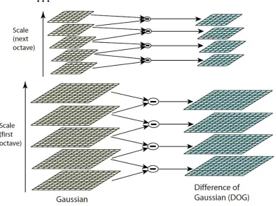
The scale space of an image is defined as:
L(x, y, σ) =G(x, y, σ)∗I(x, y) (2.1)
WhereGis a Gaussian filter andIis the input image. The difference of Gaussians (DoG)
is then calculated by:
Figure 2.1: This figure shows the difference of Gaussian method used to find scale space
extrema. This image was taken from [15]
Wherekis a multiplicative factor. After a sufficient number of scales has been found,
the scale that corresponds to 2σ is downsampled by 2 and the DoG calculation is
com-puted for that image. An example of an efficient method for calculating DoG of scale
2.2.2
Local Image Descriptor
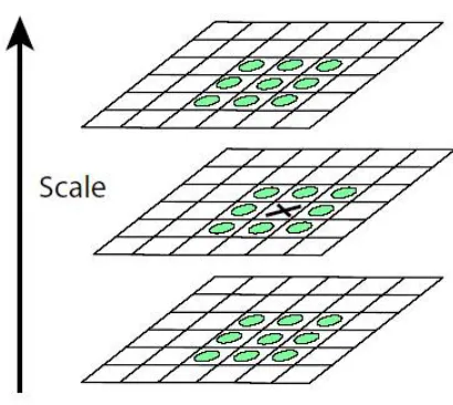
Figure 2.2: Illustation of computing local extrema
At each frame in scale-space, each point is compared to the eight nearest neighbors and
then compared to the nine nearest neighbors in the scales above and below. A graphical
example of this can be seen in Figure 2.2. If any of these are greater than or less than that
of the point in question then that point is not a local extrema.
Removal of edge dependent image descriptors is necessary for accurate local
descrip-tors at different scales because of shadow illumination differences. This is accomplished
by first evaluating the eigenvalues of the Hessian matrix H from computing Trace(H)
and Det(H)seen in equation 2.3 of the DoG images.
H=
Dxx Dxy
Dxy Dyy
Trace(H)2
Det(H) <
(r+ 1)2
r (2.4)
From equation 2.4, ifr is below a certain threshold, eliminate the local extrema,
corre-sponding to the point calculated from equation 2.3.
The remaining image pixel locations are scale invariant keypoints, used for image
matching and point correspondences between images. A nearest neighbor algorithm is
generally used to find point correspondences between images for recognition and
match-ing. The SIFT method was implemented for sequencing by finding the greatest number
of matched keypoints. The results can be seen in Section 4.4.
2.3
Object Recognition
This section discusses recognition methods used for computer vision that take into
ac-count varying pose angle views. These methods concentrate on proper feature space
rep-resentation to include the randomness of an object view angle presented in an image. The
methods of [16–18] propose dimensionality reduction to approximate the image data by
creating a database for matching. The research of are a couple of the first applications
of PCA to computer vision. The methods of [17–19], use a PCA reduced space
mani-fold for matching image sequences. Laplacian eigenmaps is a more recently developed
method used for transforming a reduced space manifold into clusters for classification.
2.3.1
Recognition and Varying Pose
The method of Murase et al. [17] uses PCA to find image features and to reduce the
amount of image data for storage. This is a supervised learning method that attempts to
classify objects with varying pose. To achieve this two feature spaces are needed. One
is the universal object eigenspace and the other is the object pose eigenspace. The image
data used for the object pose space contains many objects at monotonically changing
view angles. The illumination angle is controlled by a machine, but varies with object
pose. The data used for the universal eigenspace is composed of all objects and pose data.
Classification starts by finding the object in universal object eigenspace using minimum
distance. The pose is found in a similar manner using the pose space. This method is
similar to the proposed method for this thesis. The main difference is this thesis uses a
pose manifold in eigenspace for unsupervised object pose sequencing. The sequencing is
used to find the position of the current camera view to that of the next view.
Moghaddam and Pentland [18] describe a search method using a large facial image
database in reduced feature space to find the closest match to the input face. Preprocessing
is done to the facial image in order to obtain consistency throughout the datasets for
comparison. The preprocessing consists of face flattening and centering. The principal
component projections are computed for dimensionality reduction and feature extraction
of the facial images. The search is conducted by minimizing the distance from feature
space metric (DFFS), which is the euclidean distance in the eigenface space. The pose
angle is identified using a training set of faces at varying poses, then the face is matched to
the face of that pose similar to the method of [17]. The differences are the preprocessing
recognition. It is important to note that this thesis does not use templates for key feature
selection for tracking. More recent research [2, 13, 14], addresses object recognition at
various poses using SIFT rather than PCA or a combination seen in [3]. These algorithms
do not address the issue of sequencing the pose order of multiple images.
2.3.2
Laplacian Eigenmaps
Laplacian eigenmaps is a new field of research in machine learning, computer vision and
recognition. It is an unsupervised method used for clustering. Laplacian eigenmaps are
applied to a higher dimensional manifold to reduce the space for clustering in a lower
dimensional space.
Wij =exp
−kxj −xik t
(2.5)
The process begins with manifoldX = [xi. . .xk]withk being the number of vectorized
images in X. A weight matrixWij is computed using the heat kernel given in equation
2.5. Wij is computed from when xi and xj, is an edge, or nearest neighbor, otherwise
a zero is placed in Wij in the corresponding matrix location. The process is repeated
until all points in the manifold have been visited. Two parameters must be chosen for the
weight map:
1. The value oft.
2. The number of edges to be used in the computation.
Ly=λDy (2.6)
The Laplacian is defined as,L=D−W whereDis a diagonal weight matrix calculated
from equation 2.5, such that Dii =
P
j
Wij. The eigenmap is computed by solving the
From equation 2.6, the eigenvalue with the lowest value corresponding to the matrix
of eigenvectorsyis the solution to the Laplacian matrix. The rank of the Laplacian matrix
indicates the number of eigenvectors yielding a trivial solution. For this reason, care must
be taken when selecting the eigenmaps.
2.3.3
Manifold Learning
Constrained manifold learning has been used to estimate camera pose, generate matched
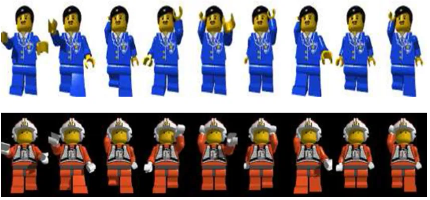
animations, and to match human lip movements. An example for manifold matching
[image:23.612.110.539.364.564.2]from [19] can be seen in Figure 2.3.
Figure 2.3: This figure shows an example of matching animations of a toy figure
This is a non-iterative method using the concept of diffeomorphism to generate a
map between two manifolds x ∈ X and y ∈ Y. In mathematics, diffeomorphism is
manifolds are generated in PCA space from images xandy, such that X andY are the
manifold spaces. Learning manifold maps in [19] is based on computing a local manifold
smoothness. Manifold smoothness in PCA space is used in this thesis as well. Chapter 3
will discuss this in more detail.
2.3.4
Image Feature Distributions
One method described in [14, 20] uses the earth movers distance (EMD) to match images
from a database. The EMD operates on image feature distributions and is described as the
amount of work needed to match one histogram of image featuresxi to anotheryj. This
method is useful for matching overall image content, such as matching similar background
scenes and characters. However it does not discriminate fine spatial features to capture
and order the motion in the images. This is due to the loss of spacial information when
binning pixels into a histogram. Furthermore, histogram matching needs high variability
in the pixel distributions not considering the variation of an entire data set.
2.4
PCA Solution for Pose Ordering
This section is intended to explain the problem of pose ordering using PCA. A problem
description has been formulated to explain why PCA is chosen as a feature space and the
benefits that PCA can offer. The benefits provided will expose it’s drawbacks for certain
2.4.1
PCA Description
The problem for ordering random object poses is viewed as a problem in pose recognition.
This problem is primarily solved using principal component analysis (PCA) because of
it’s simplicity. Moreover, computing PCA on sequences of object poses produces distinct
geometry in eigenspace. This occurs because of the properties and assumptions of PCA:
1. Dimensionality reduction
2. Linear combination of feature components
3. Gaussian distributed feature components
4. Orthogonality of feature components
5. Linear transformation
PCA offers dimensionality reduction for developing large databases of training data
for recognition. Dimensionality is reduced by minimizing the mean square error over the
dataset. Feature selection is performed by choosing a linear combination from the data
containing the maximum variance. The maximum variance across the data set satisfies the
minimum mean square error criteria for embedding the data in a reduced space. This is an
important aspect to any pattern recognition problem. The eigenvectors and eigenvalues
of the autocorrelation matrix of the data correspond to the orthogonal basis function and
the decorrelated variance,respectively. The features are a result from the minimization
of the error of the projection space to the data known as the eigenspace. The number of
The criteria for dimensionality reduction using PCA assumes the data is Gaussian
distributed with an unbiased mean and variance. PCA is an optimal embedding technique
for Gaussian distributed data, because it captures the mean and variance as defined by a
Gaussian probability distribution. Multimodal data does not follow the know equations
for the mean and variance. This breaks the assumption of an optimal embedding space
for minimizing the mean square error with maximum variance. Important data is now lost
making it impossible for correct classification. However, for image processing purposes
used in this thesis, the manifold from the assumed Gaussian distribution is of interest.
This implies that PCA is optimal for data embedding and comparison.
The optimal embedding space, as stated previously, are the eigenvectors of the
auto-correlation matrix of the image data set. Eigenvectors are known for the property of being
orthogonal to each other. Having an orthogonal space means that each basis dimension is
uncorrelated to the another. This is characteristic of the diagonalization of the
autocorre-lation matrix. This is another source of data loss because linear mixtures may exist within
a single principal component. However, the property is desirable when the objective is to
indiscriminately extract all spatial variant features across the image data set. It comes to
be a problem when specific image features are desired other than the maximum variance.
This thesis shows that neither classification nor clustering is a desired technique for image
pose ordering. Rather the pose ordering method is seen as a process of sequencing images
by the arrangement of the PCA representation of the unordered image set. This offers a
solution to ordering under the condition that it is a scatter of points producing a structured
manifold in eigenspace.
The linearity of PCA is a highly desired characteristic for ordering random object
of each pixel over an entire set of images, is independent of the order of the images.
This implies the input order of the image sequence does not dictate the structure of the
manifold and the multidimensional eigenspace is the same regardless of the random order
of images.
2.4.2
PCA for Pose Recognition
The idea of using PCA for pose ordering comes from the previous work done in
super-vised pose recognition (see Section 2). This work [17] shows results of multidimensional
manifolds in eigenspace for each object at different poses and different illumination. Each
point in eigenspace represents an object pose. As the manifold trajectory is traced to each
image the pose angle changes. The minimum distance to the object space and the
min-imum distance to the pose space is the solution for recognition of the object and pose
view respectively. The shape and the resolution of the manifold will dictate the ordering
results. Increasing the number of image views with varying illumination would achieve a
more accurate pose sequencing. If not, a more sophisticated algorithm will be needed for
Chapter 3
Theoretical Development of the Pose
Ordering Algorithm
3.1
Principal Component Analysis
The rational for using Principal Component Analysis (PCA) has already been provided in
Section 2.4.1. The next section will help to explain the how PCA is applied to a sequence
of images for the purpose of ordering view-angles. Furthermore, this section will show
image examples and explain eigenposes. These are the basis functions used for computing
the geometrical configuration of a set of random object poses. A treatment of PCA can be
found in [21].
3.1.1
Mathematical Description of Proposed Method
Each image xi of size M × N in the randomly captured sequence is formed into an
X = [x1, . . . ,xK] of random object poses. Normalization is not done across the image
set. This way, illumination and shadows are preserved as these are seen as features for
ordering poses. The next step is to calculate the eigenspace of the random set. The
eigenspace basis matrix E is composed of the L largest corresponding eigenvalues for
someL. The square matrixQ = XXT is computed and singular value decomposition is
done such that:
Q=ETΛE (3.1)
WhereΛis the diagonal matrix of eigenvalues.
g(xi) =xTi E (3.2)
The projectiong(xi), of sizeL×1, of the image onto the eigenspace is then calculated
and used as the feature space.
3.1.2
“Eigenpose” Analysis
The eigenvectors were plotted to visualize the dominant features for some test objects.
These plots can be seen in Figures 3.1 and 3.2. The term “eigenposes” was taken from
the term “eigenfaces” in [18]. The first ten principal components eigenvector images are
Figure 3.1: Eigenvectors for an object with less details
Figure 3.2: Eigenvectors for an object with more details
Whereeiis the unit eigenvector found in theithcolumn ofEandλiis theithdiagonal
component of Λ seen in equation 3.1. After this is done, the vector must be rearranged
into an image given width and height dimensions.
Eigenposei =pλiei (3.3)
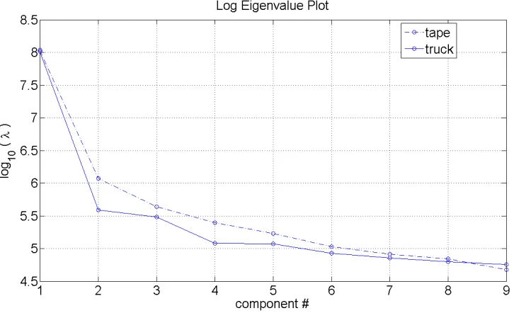
truck images can be seen in Figure 3.3 plotted on a logarithmic scale. It can be noted that
[image:31.612.138.501.198.419.2]the eigenvalues drop off faster in the truck images than in the tape images.
Figure 3.3: Base ten logarithm of the eigenvalues associated with the first nine
eigenvec-tors seen in Figures 3.1 and 3.2
The number of principal components utilized can be determined from equation 3.4
seen in [17].
I = PL
i λi
PM N
i λi
(3.4)
The output,I, is the fractional amount of information that is explained by the variance in
the image set. The information measure should be close to one. For each object tested,I
was computed to represent 99% of the information from the variance and can be seen in
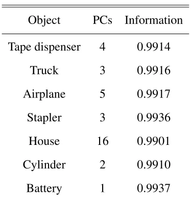
Object PCs Information
Tape dispenser 4 0.9914
Truck 3 0.9916
Airplane 5 0.9917
Stapler 3 0.9936
House 16 0.9901
Cylinder 2 0.9910
[image:32.612.230.417.121.320.2]Battery 1 0.9937
Table 3.1: Information measurement for each object tested
Table 3.1 shows the number of principal components needed to represent 99% of
the information from the variance. Section 4.2.3 will show experimental results for the
amount of information needed.
3.2
Object Pose Ordering
The proposed approach for ordering images is an iterative process. LetSj andΘj be the
set of unordered and ordered images at iterationj, respectively. To begin,S0is the entire
set of unordered images andΘ0 is the empty set of ordered images. At iterationj = 1, a
randomly chosen image is labeledx1 and moved fromS0 toΘ0, yieldingS1andΘ1. For
j ≥2an imagexj is moved fromSj−1toΘj−1such that:
xj =argmin
x∈Sj−1
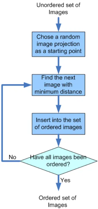
Figure 3.4: Block diagram of the single camera ordering algorithm implemented
Thus, the ordering algorithm picks from the unordered set, the image closest to the last
ordered image in eigenspace. The diagram in Figure 3.4 shows the algorithm for single
camera ordering. Once the images have been ordered using the minimum separation,
a confidence measure is computed using local curvature along the trajectory (called the
Letdsj be the vector:
dsj =g(xj)−g(xj−1) (3.6)
The cosine of the angle between the vectors is the correlation coefficient:
cos(θj) =
dsTjdsj−1
kdsjk kdsj−1k
(3.7)
The difference between vectors is then computed by subtracting the two vectors. The
difference equation is an approximation to the second order derivative for curvature:
κj =
q
(dsj−1 −dsj) T
(dsj−1−dsj) (3.8)
The confidence in ordering metric is given by:
cj =κj(1−cos (θj)) (3.9)
3.2.1
PCA Based Distance Metrics
Other PCA based distance metrics were tested for the use with pose ordering [22]. For
these equations gi(x)represents each principal element of the projection transformation
from equation 3.2.
• Euclidean distance:
d(g(xj−1),g(x)) = s
X
i
(gi(xj−1)−gi(x))
2
(3.10)
• Angle based distance:
d(g(xj−1),g(x)) =−cos(g(xj−1),g(x)) (3.11)
= P
i
gi(xj−1)gi(x)
P
i
gi(xj−1)2P
i
• Mahalanobis distance:
d(g(xj−1),g(x)) = X
i
zigi(xj−1)gi(x) (3.13)
wherezi = 1/λi
• Manhattan distance:
d(g(xj−1),g(x)) = X
i
zi|gi(xj−1)−gi(x)| (3.14)
wherezi = 1/λi
The distance metric that produced the best results was the eucleadian distance. This
is because it takes into account the geometrical separation and preserves the significance
of the principal component transformation. The other metric either normalize the
signif-icance of each component or normalize the distance, which makes it difficult to compare
3.2.2
Confidence Metric
Figure 3.5: The vector representation of the confidence measure
The confidence metriccjattempts to use a combination of three local image projections to
measure the alignment and the curvature. The alignment is equivalent to the congruence
coefficient across three images and is equal to zero when they are in a straight line. The
curvature acts as a weight across the combination of the three images. A low confidence
measure indicates the images are changing slowly and pose classification is more accurate
in this region and a high measure of confidence means the images are changing erratically.
For this confidence measure, a low value is desirable to indicate correct ordering. The
3.2.3
Development of the Confidence Metric
(a) Correct pose manifold trajectory
(b) Incorrect pose manifold trajectory
Figure 3.6: Comparison of the correct manifold and the incorrect manifold
The development of the confidence metric was motivated by the problem of detecting
errors in ordering. A geometrical feature was chosen as a metric because of the
produced by direct computation of PCA on the order image sequence. Figure 3.6(b) was
produced using the ordering algorithm seen in Figure 3.4. Differential geometry defines
the trajectory of a moving particle in space to be γ(t). This is the representation of the
object manifold. Therefore, the formal definition of curvature is given as:
κ(t) = γ
00
(t)
(3.15)
For the purposes of this thesis, the difference equation of this measure is used and was
(a) Images 1-10 corresponding to the first two errors
(b) Images 21-30 corresponding to the third error
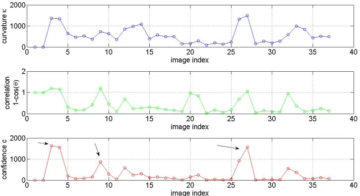
Figure 3.8: Top: Curvature,Middle: one minus correlation,Bottom:confidence. These
were calculated after pose ordering. The arrows point out the errors observed in pose
ordering
The two types of metrics chosen for ordering are curvature,κj, and correlation, cos(θj),
as described in the previous section. Plots of these metrics for a test object are shown in
Figure 3.8. The single camera algorithm used to produce the results is seen in Figure 3.4.
The figure is intended to show how the combination of the two metrics perform the task of
recognizing errors within the single camera ordering algorithm. The errors are referenced
by the arrows in Figure 3.8. The images that correspond to these errors can be seen in
Figure 3.7(a) and 3.7(b). It is important to note that the confidence is calculated using
three images, therefore each point represents images indicesj−2,j−1, andj.
It is difficult to observe, by an untrained eye, the errors in pose ordering of Figures
the front and back views of the object.
3.3
Two Camera Ordering with Confidence
This section is intended to explain, in detail, the confidence metric utility integrated into
the two camera architecture. The main idea is to use the confidence metric to correct the
errors found when ordering using the minimum distance. To achieve this, a second camera
has been included in the experiment. This second camera creates additional information
used for the pose ordering algorithm.
3.3.1
Two Camera Configuration
Figure 3.9: Two camera configuration used in the experiment
The two camera configuration can be seen in Figure 3.9. The two cameras are placed90◦
apart in viewing angle in an attempt to gain more salient object features and eliminate the
180◦errors seen in Figure 3.7, images 9 and 10. These errors are because the pose space
of the object is dominated by side views. Physically the side view is larger containing
variance maximization feature extraction. Some eigenvectors were seen in Figures 3.1
and 3.2.
3.3.2
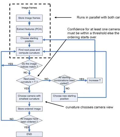
Implementation of the Confidence Metric
The single camera method is extended to the case where two synchronized cameras are
available. Since the cameras are synchronized, we can compare the time indices of each
camera. By independently ordering each camera’s images, it can be said that if the time
indices do not match, then an error in ordering has occurred. The difficulty lies in
deter-mining automatically which camera view is more likely to have incorrectly ordered the
images. This is done by comparing the confidence cj developed in the previous section
and time indices of each camera to determined if an error has occurred and which camera
has the lower confidence of error. Ifccamera1
j > ccameraj 2 then camera two is chosen for
the next view and vice versa. A block diagram for the algorithm described can be seen in
3.3.3
Confidence Thresholding
A large confidence metric is intended to exploit problem areas for pose ordering in the
ob-ject manifold. What happens when both confidence values are significantly large?
Con-sider a value T as a threshold to detect outliers in the confidence values. Any
confi-dence value greater than T is an outlier. The ordering method is designed such that: if
ccamera1
j > c camera2
j andc camera2
j > T, then reject the hypothesis that camera two is the
correct next pose. This is because the confidence in ordering is not high.
µ= 1
N
X
j
ccamerak
j (3.16)
and the standard deviation by:
σ = 1
N −1 X
j
ccamerak
j −µ
2 !1/2
(3.17)
andN is the number of confidence values (number of images−2). This can be seen in
Figure 3.11.
T =µ+σ (3.18)
To initialize the confidence metric threshold, all confidence values are computed for a
single image. Next, a threshold is chosen from the statistics of the confidence distribution.
Figure 3.11: Histogram of the confidence values for the two cameras. The threshold and
mean are shown as dotted lines.
If the camera hypothesis for the confidence values is rejected, then the threshold is
increased by a factor (10%is used in the results). By increasing the threshold, the method
will eventually converge to a pose ordering solution. This step can be seen in the block
Chapter 4
Results
4.1
Procedure
The results were obtained from videos taken of many objects on a turntable. The first test
was pose sequencing with a single camera, and the second test was pose sequencing with
two synchronized cameras. Please refer to Section 3.3.1 for two camera configuration.
The video sequence was scrambled in MATLAB using a uniform random number
gen-erator. The known video sequence is used to help with assessing the results of ordering.
The random number set is used to produce an equal distribution for the full rotation of
the object. This means that no views are repeated and if a histogram of pose angle was
created, then there would be only one count per bin. A set of images that includes a full
rotation of the object ensures that the first and last images are connected in eigenspace. It
also makes error counting and validation of the ordering simpler. The video frame rate is
16 frames/sec and the number of poses in a set varies from 30 to 37 depending on the
This is done to accommodate the large size of the covariance matrix. The formulation
of the covariance matrix for PCA is not normalized by illumination. It is thought that
illumination is a feature for recognition of objects and scenes used by human vision.
The error rate for object ordering is calculated manually by visual inspection of the
images and counting the number of incorrectly sequenced images. By definition, an error
occurs if the next pose does not correspond to the current pose for the set of images. Error
rate is calculated for the entire set by summing the total number of errors and dividing by
the number of images in the set.
Object Single Camera Two Cameras Gain
Tape dispenser 17.0% 0.9% 16.1%
Stapler 9.1% 0.3% 8.8%
Truck 6.7% 0.3% 6.4%
House 3.0% 0.9% 2.1%
Airplane 1.5% 0.3% 1.2%
Cylinder 0.6% 0.0% 0.6%
Battery 0.3% 0.0% 0.3%
Table 4.1: Error Rate of Ordering Various Objects
Objects without distinct features have failed to order properly in the single camera
case because of the similarity of views. These objects without saliency are referred to in
Table 4.1 as the tape dispenser and the truck. For these types of objects, the recognition
Figure 4.1: Example of errors in the pose manifold reconstruction
Most of the errors occur where the manifold begins to wrap around itself and become
tangled. This can be shown in Figure 4.1, where the circled region represents the problem
area when the next angle-view is not the minimum distance. The dotted line shows the
errors for ordering with a single camera. The solid line in Figure 4.1 shows the correct
Figure 4.2: This figure plots both manifolds from camera 1 and camera 2, and shows the
errors in dotted lines and correctly ordered in the solid lines. The confidence value is also
printed for the last manifold connection made
A depiction of how the confidence measure helps to select the correct camera for
viewing can be seen in Figure 4.2. The figure shows the camera whose manifold is chosen
contains the section that is the most flat and is the minimum distance across images. In
the example in Figure 4.2, camera one has made an error and camera two is chosen as the
Figure 4.3: Results for two camera ordering
Figure 4.3 shows an example of the confidence selecting between camera one and
camera two for front and side views of the tape dispenser. The images displayed in Figure
4.3 are seen from the perspective of camera one. As the front view appears, camera one
4.2
Pose Ordering Error Analysis
Trial # Single Camera Two Cameras
1 5 2
2 4 0
3 7 0
4 5 0
5 6 0
6 7 0
7 5 1
8 7 0
9 5 0
10 5 0
Avg 5.6 0.3
Var 1.04 0.41
[image:51.612.213.434.183.521.2]Avg error 17.0% 0.9%
Table 4.2: Number of errors for the tape dispenser
In trial seven the single error can be classified as a depth perception error, and can be seen
Trial # Single Camera Two Cameras
1 2 0
2 5 1
3 2 0
4 0 0
5 2 0
6 3 0
7 2 1
8 2 0
9 3 0
10 2 0
Avg 2.3 0.1
Var 2.33 0.11
Avg error 6.7% 0.3%
Trial # Single Camera Two Cameras
1 2 0
2 2 1
3 4 0
4 2 0
5 3 0
6 3 0
7 4 1
8 3 0
9 4 0
10 3 0
Avg 3.0 0.1
Var 0.6 0.09
Avg error 9.1% 0.3%
Trial # Single Camera Two Cameras
1 0 0
2 0 0
3 0 0
4 3 1
5 0 0
6 0 1
7 3 0
8 0 1
9 1 0
10 3 0
Avg 1.0 0.3
Var 1.8 0.21
Avg error 3.0% 0.9%
Trial # Single Camera Two Cameras
1 1 0
2 0 0
3 0 0
4 0 0
5 1 1
6 0 0
7 0 0
8 0 0
9 1 0
10 2 0
Avg 1.0 0.3
Var 1.8 0.21
[image:55.612.211.435.121.461.2]Avg error 3.0% 0.9%
Trial # Single Camera Two Cameras
1 0 0
2 0 0
3 0 0
4 1 0
5 0 0
6 0 0
7 0 0
8 0 0
9 1 0
10 0 0
Avg 0.2 0.0
Var 0.16 0.00
[image:56.612.213.433.122.461.2]Avg error 0.6% 0.0%
Trial # Single Camera Two Cameras
1 0 0
2 0 0
3 0 0
4 0 0
5 1 0
6 0 0
7 0 0
8 0 0
9 0 0
10 0 0
Avg 0.1 0.0
Var 0.09 0.00
[image:57.612.213.435.123.463.2]Avg error 0.3% 0.0%
Table 4.8: Number of errors for the battery
This section shows tables of error rates for each object tested. Table 4.1 contains
a summary of all the object results, while Tables 4.2-4.8, contain results for individual
trials for each object. A trial is a different randomization of poses used for each object.
This includes different starting points for the algorithm and different angled-views taken
4.2.1
Single Camera
Figure 4.4: Tape dispenser images 1-10
[image:58.612.167.484.407.583.2]Figure 4.6: House images 11-20
This section will show image examples in the single camera ordering process. The
pre-vious section shows the errors in terms of the eigenspace representation. This section
displays errors that correspond to image ordering. Figure 4.4 shows 4 errors occuring in
the sequence of ten images. These errors are caused by the confusion between the front
and rear views of the object. The confusion is caused by PCA dimensionality reduction
and it’s inability to select the required features to distinguish between these views. Some
of these object views require certain details that become eliminated when using PCA.
This will be shown in the reconstructed images using nine principal components. These
Figure 4.7: Image reconstruction using the first nine principal components for the tape
dispenser images. The numbers in parenthesis represent the indices from the original
video
Figure 4.8: Image reconstruction using the first nine principal components for the truck
[image:60.612.110.541.376.596.2]Figure 4.9: Image reconstruction using the first nine principal components for the house
images. This image can be compared to that in Figure 4.6
The inability of PCA to choose the correct features can be seen in the reconstruction of
the image sequences in Figures 4.7-4.8. These views look undistinguishable to a trained
human eye. To verify the validity of ordering, the frame indices from the original video
sequence are shown in parenthesis. These indices are referred to as, in Section 4.1, the
4.2.2
Two Cameras
Figure 4.10: Example of a depth error induced from camera 1 confidence
This section will show image examples of how two camera ordering improves single
camera ordering and the types of errors seen in using two cameras. Figure 4.10 show
results of two camera ordering with a depth perception error. The error is a result from
camera one similarity and camera two’s inability to distinguish between front views. The
view from camera two cannot be seen, but it is known that it is facing 90◦ apart from
camera one which is facing the side. The two camera configuration is intended to switch
4.2.3
Eigenvalues v. Error Rate
Figure 4.11: Number of principal components versus average error for an object. The
standard deviation has been plotted for each trial.
Figure 4.11 represents the average error of pose ordering given a number of principal
components. The average error has been taken over ten trials. Each trial has been given
a different set of poses for the same object. From the plot in Figure 4.11 the optimum
number of eigenvalues is nine. This is where the error rate reaches a limit and cannot
be improved by adding more principal components. There is actually a slight decline
in performance using higher dimensions. As mentioned in Section 3.1.2, 99% of the
information explained by the variance is not enough to do accurate pose sequencing for
4.3
Laplacian Eigenmaps
In the previous section the object manifold was shown along with the analysis of errors
in eigenspace. The Laplacian eigenmap method acts on the reduced space images of the
manifold seen in the previous section. This method uses a Laplacian kernal to solve the
eigenvalue problem seen in Section 2.3.2 on Laplacian eigenmaps. This section shows
the results of the Laplacian eigenmap on the object manifold are clusters of image poses
[image:64.612.114.536.327.594.2]in the Laplacian eigenspace.
Figure 4.13: Laplacian eigenmap method t = 500
[image:65.612.125.524.427.653.2]Figure 4.15: Ordered images 11 - 20 using Laplacian eigenmaps, t = 100
The first twenty ordered images, from the clusters seen in Figure 4.12, can be seen in
in figures 4.14 and 4.15. The transition between pose clusters is indicated by the circled
images. This is the region where a jump must be made from one pose cluster to another
from the previously ordered image to the closest point in the next cluster. This is an
undesired result because it is difficult to assess whether the pose is in the correct sequence.
The Laplacian eigenmap method is primarily an unsupervised clustering algorithm to find
a geometric solution to multidimensional data. Although this is a powerful method for
unsupervised learning, it is not very useful for sequencing because the smooth manifold
Figure 4.16: Single camera pose results for comparing the results of Laplacian eigenmaps
A comparison of the single camera method to the Laplacian eigenmaps helps to
con-vey the idea of a smooth manifold. The types of errors from each method are distinctly
different. Laplacian eigenmaps show errors of discontinuous views between the clusters
and confusion of similar views resulting from dimensionality reduction. The PCA method
contains errors just that of confusion of similar views due to dimensionality reduction.
Figure 4.16 shows a smooth transition from front to intermediate view and intermediate
to side views. The image sequence in 4.15 shows a jump from front views to side views
that are apart approximately90◦ in rotation. This sequence does not exhibit any transition
to intermediate views before side views. The single camera PCA method clearly shows
4.4
SIFT Results
Figure 4.17: Results of the SIFT implementation for the tape dispenser images
Figure 4.18: Results of the SIFT implementation for the truck images
The application of SIFT was found to not be useful for object pose ordering because
[image:68.612.113.537.407.598.2]sim-ilarities around a 360◦ view confused the keypoint matching metric into finding many
unlike views. This is a result of SIFT’s inability to recognize objects in a scene
exceed-ing a certain angled view. The illumination differences also cause too much confusion
Chapter 5
Conclusion
5.1
Summary
This paper has outlined and specifically designed a method for ordering image poses of
an object using a single or multiple camera architecture. PCA has been used as a basis
for the algorithm because of its dimensionality reduction and feature extraction
proper-ties. Moreover, PCA has been used in multiple research applications for pose and object
recognition (see Section 2). Data has been presented that shows the method from single
camera ordering can be improved by adding an additional camera. A confidence metric
has been developed that detects errors in ordering. The confidence metric is applied in
eigenspace and allows for the fusion between two or multiple cameras. The fusion can be
5.2
Future Work
Other applications for pose ordering such as path planning, which is used for
control-ling and monitoring moving objects, could be seen as a possible application. This is
thought because the path of a vehicle or object that traverses a trajectory is a
multidimen-sional manifold [23]. By using video frames, one could also embed a path into a reduced
eigenspace. The manifold could be used to predict the controls of a vehicle [24]. The idea
Bibliography
[1] A. Newman, “Face-recognition systems offer new tools, but mixed results,” New
York Times, 2001.
[2] D. G. Lowe, “Distinctive image features from scale-invariant keypoints,”
Interna-tional Journal of Computer Vision, 2004.
[3] Y. Ke and R. Sukthankar, “Pca sift: A more distinctive representation for local image
descriptors,” IEEE Conference on Computer Vision and Pattern Recognition, 2004.
[4] J. Massaro and R. Rao, “Object pose ordering,” IEEE Conference on Acoustics,
Speech, and Signal Processing, 2009.
[5] S. O’Dwyer, P. Lewis, and J-P. Muller, “An application of stereomatching to the
problem of geo-referencing historical air photos,” IEEE Conference on Remote
Sensing, 2003.
[6] M. Potuckova, “Image matching and it’s application to photogrammetry,” Ph.D.
[7] L. Aryananda, “Online and unsupervised face recognition for humanoid robot:
To-ward relationship with people,” IEEE- RAS International Conference on Humanoid
Robots, 2001.
[8] W. Seales and O. Faugeras, “Building three dimensional object models from
se-quences,” Computer Vision and Image Understanding, vol. 61, no. 3, pp. 308–324,
1995.
[9] A. Bottino and A. Laurentini, “Shape-from-silhouette when the relative position of
the object is unknown,” TPAMI, vol. 25, no. 11, pp. 1484–1493, 2003.
[10] K. Chueng, S. Baker, and T. Kanade, “Visual hull alignment and refinement across
time: A 3d reconstruction algorithm combining shape-from-silhouette with stereo,”
IEEE Conference on Computer Vision and Pattern Recognition, 2003.
[11] T. Joshi, N. Ahuja, and J. Ponce, “Structure and motion estimation from dynamic
silhouttes under perspective projection,” Int. Journal on Computer Vision, pp. 290–
295, 1995.
[12] M. Brown R. Szeliski and S. Winder, “Multi-image matching using multi-scale
oriented patches,” IEEE Conference on Computer Vision and Pattern Recognition,
2005.
[13] M. Brown and D. G. Lowe, “Unsupervised three dimensional object recognition
and reconstruction in unordered data sets,” IEEE Conference on 3D Imaging and
[14] K. Grauman and T. Darrell, “Efficient image matching with distributions of local
invariant features,” IEEE Conference on Computer Vision and Pattern Recognition,
vol. 2, no. 20, pp. 627–634, 2005.
[15] D. G. Lowe, “Object recognition from local scale-invariant features,” Proc. of the
International Conference on Computer Vision, pp. 1150–1157, 1999.
[16] D. Beymer, “Face recognition underying pose,” MIT Artificial Intelligence
Labora-tory, , no. 89, 1993.
[17] H. Murase and S.K. Nayar, “Learning and recognition of 3d objects from
appear-ance,” Int. J. of Comp. Vis., vol. 14, pp. 5–24, 1995.
[18] B. Moghaddam and A. Pentland, “Probabilistic visual learning for object
represen-tation,” TPAMI, vol. 19, no. 7, pp. 696–709, 1997.
[19] J. Ham, I. Ahn, and D. Lee, “Learning a manifold-constrained map between image
sets: applications to matching and pose estimation,” IEEE Conference on Computer
Vision and Pattern Recognition, 2006.
[20] Y. Rubner, C. Tomasi, and L. J. Guibas, “A metric for distributions with
applica-tions to image databases,” Proc. of the IEEE International Conference on Computer
Vision, 1998.
[21] R. Duda and P. Hart, Pattern Classification, Wiley-Interscience, New York, NY, 2nd
edition, 2001.
[22] V. Perlibakas, “Distance measures for pca-based face recognition,” Pattern
[23] C. Leung, S. Huang, and G. Dissanayake, “Active slam using model predictive
con-trol and attractor based exploration,” Inter. Conf. on Intelligent Robots and Systems
IEEE/RSJ, pp. 5026–5030, 2006.
[24] E. W. Frew, D. Lawrence, C. Dixon, J. Elston, and W. J. Pisano, “Lyapunov
guid-ance vector fields for unmanned aircraft application,” Proc. of American Control
Conference, pp. 371–376, 2007.
[25] A. Kurdila, M. Nechyba, R. Prazenica, W. Dahmen, P. Binev, R. DeVore, and
R. Sharpley, “Vision-based control of micro-air-vehicles: progress and problems
in estimation,” 43rd IEEE Conference on Decision and Control, vol. 2, pp. 1635 –