Theses Thesis/Dissertation Collections
2011
Establishing parameters for problem difficulty in
permutation-based genetic algorithms
Adam Nogaj
Follow this and additional works at:http://scholarworks.rit.edu/theses
This Thesis is brought to you for free and open access by the Thesis/Dissertation Collections at RIT Scholar Works. It has been accepted for inclusion in Theses by an authorized administrator of RIT Scholar Works. For more information, please [email protected].
Recommended Citation
for Problem Diculty
in Permutation-Based
Genetic Algorithms
byAdam F. Nogaj
A Thesis Submitted in Partial Fulllment of the Requirements for the Degree of Master of Science
in Computer Science
Supervised by
Professor Dr. Roger S. Gaborski Department of Computer Science
B. Thomas Golisano College of Computing and Information Sciences Rochester Institute of Technology
Rochester, New York October 2011
Approved by:
Dr. Roger S. Gaborski, Professor
Supervisor, Department of Computer Science
Dr. Peter G. Anderson, Professor Emeritus Reader, Department of Computer Science
Dedication
To my parents, Larry and Colleen Nogaj,
to my grandparents, Wilfred and Susan Finn, and Stan and Rena Nogaj, and to my amazing wife, Lisa,
who have surrounded me with more kindness, support, generosity, and love than I could ever begin to describe.
Acknowledgments
First and foremost, I would like to thank RIT Department of Computer Science Graduate Coordinator Dr. Hans-Peter Bischof and my thesis committee, especially
Dr. Peter Anderson, for their ongoing patience and willingness to help guide and support me throughout my thesis. I would also like to thank the math and computer science faculty at SUNY Fredonia, especially Dr. Ziya Arnavut, for
Abstract
Establishing Parameters for Problem Diculty in Permutation-Based Genetic Algorithms
Adam F. Nogaj
Supervising Professor: Dr. Roger S. Gaborski
This thesis examines the performance of genetic algorithm (GA) crossover techniques within two problems: n-queens with poison (NQWP) and processor scheduling (PS).
Contents
Dedication . . . ii
Acknowledgments . . . iii
Abstract . . . iv
1 Introduction . . . 1
1.1 Genetic Algorithms . . . 1
1.2 Permutation-Based Genetic Algorithms . . . 6
1.3 Ordered Greed . . . 7
1.4 Additional Denitions and Clarications . . . 8
1.4.1 Crossover Techniques . . . 8
1.4.2 Problems, Runs, Tests, and Experiments . . . 8
1.4.3 Diculty . . . 9
1.4.4 Constraint Density . . . 9
1.5 Practical Approach . . . 10
1.6 Visual Representation of Data . . . 12
2 Techniques . . . 13
2.1 Crossover Methods . . . 13
2.1.1 Cycle Crossover (CX) . . . 14
2.1.2 Order Crossover (OX) . . . 15
2.1.3 Merging Crossover (MOX) . . . 17
2.1.4 Partially-Mapped Crossover (PMX) . . . 19
2.1.5 Signature Crossover (SX) . . . 21
2.1.6 Hybrid Crossover (HX) . . . 23
2.1.7 Randomizing Individuals . . . 23
2.1.8 Null Crossover . . . 24
2.1.9 Greedy Approaches . . . 24
2.1.9.1 GREEDY-1 . . . 24
2.1.9.2 GREEDY-2 . . . 24
2.1.9.3 GREEDY-3 . . . 25
2.2 Population . . . 25
2.3 Selection . . . 25
2.4 Deselection . . . 26
2.5 Mutation . . . 26
3 N -Queens With Poison (NQWP) . . . 28
3.1 Diculty . . . 31
3.2 Problem Representation . . . 31
3.3 Problem Set Creation . . . 32
3.4 Solution Approach . . . 32
3.5 Results . . . 33
3.5.1 Diculty . . . 35
3.5.1.1 Primary Results . . . 35
3.5.1.2 Eect of Crossover Technique on Diculty . . . 38
3.5.1.3 Eect of Population Size on Diculty . . . 38
3.5.1.4 Distribution of Dicult Problems . . . 40
3.5.1.5 GA Behavior for Dicult Problems . . . 40
3.5.1.6 Characteristics of Dicult Problems . . . 41
3.5.2 Crossover Techniques . . . 42
3.5.2.1 Primary Results . . . 42
3.5.2.2 Eect of Population Size on GA Performance . . . . 47
4 Processor Scheduling (PS) . . . 50
4.1 Diculty . . . 50
4.2 Problem Representation . . . 50
4.3 Problem Set Creation . . . 51
4.4 Solution Approach . . . 51
4.4.1 Topological Sorting . . . 52
4.4.1.1 Full Sort . . . 53
4.4.1.2 Rough Sort . . . 53
4.4.1.3 Partially Random Sort . . . 54
4.5 Results . . . 54
4.5.1 Diculty . . . 54
4.5.1.1 Primary Results . . . 54
4.5.1.2 Eect of Crossover Technique on Diculty . . . 57
4.5.1.3 Eect of Problem Size on Diculty . . . 57
4.5.1.4 Distribution of Dicult Problems . . . 58
4.5.1.5 GA Behavior for Dicult Problems . . . 58
4.5.1.6 Eect of Sorting Algorithm on Diculty . . . 59
4.5.1.7 Eect of Processor Count on Diculty . . . 60
4.5.2 Crossover Techniques . . . 66
4.5.2.1 Primary Results . . . 66
4.5.2.2 Eect of Population Size on GA Performance . . . . 70
4.5.2.3 Eect of Sorting Algorithm on GA Performance . . . 72
5 Conclusion . . . 76
5.1 Implications of Research . . . 76
5.2 Future Work . . . 77
5.2.1 Additional In-Depth Research . . . 77
5.2.2 Additional Problems . . . 78
5.2.2.1 Graph Coloring . . . 78
5.2.2.2 Classroom Seating . . . 78
5.2.2.3 Variations on N -Queens With Poison . . . 79
A Derivation of Average OX/PMX Crossover Section Size . . . 80
Chapter 1
Introduction
1.1 Genetic Algorithms
A genetic algorithm (GA) is a problem-solving methodology based on biological evo-lutionary principles. Through high school biology classes, evening news segments depicting modern advances in health and technology, and casual references in popu-lar culture, there exists a virtually ubiquitous basic understanding of the role of that DNA plays in determining a person's (or other organism's) seemingly countless char-acteristics. Combinations of just four chemical compounds within strands of DNA can contain biological instructions that inuence height, eye color, and even person-ality traits [6]. A dierent combination of the same four chemicals at a dierent part of the DNA can predispose an individual to a particular disease [7], among many other things. Additionally, it is well-understood that an ospring's DNA is created exclusively by taking portions of each parent's DNA in a largely randomized process termed chromosomal crossover [8]. An individual's DNA is also susceptible to a phe-nomenon called mutation during which it becomes altered (damaged) just slightly [9].
benecial characteristics will have the greatest opportunity to survive, and therefore, ultimately the greatest opportunity to reproduce. Through such procreation, an individual's characteristics (DNA) are passed on to children, and more generally, it suces to say that those characteristics have an increased likelihood of being exhibited in the overall population. The prevalence of such characteristics may then increase further via continued biological reproduction [10].
In GAs, an individual's DNA represents information sucient to describe a potential solution to a problem. It is often generalized that a bit string [2] (series of 1s and 0s) may be used as the language of GA DNA since at some level, anything can be represented by such binary primitives. However, realistically, any standardizable language may be utilized within a GA individual's DNA. For example, consider the problem of getting from one's house to a particular grocery store, such as the Wegmans in Pittsford, NY. DNA in this problem may be a set of instructions to be carried out at a given intersection, such as turn left, turn right, and go straight. It is easy to see that any list consisting of left turns, right turns, and go-straights does constitute a reasonable set of instructions to attempt to direct an individual toward the grocery store, even if it were randomly generated or otherwise not a very good solution. That is, there are no out of place or meaningless instructions such as bake cookies or throw a Frisbee. And if it is to be assumed that any intersection is a standard three or four-way intersection, then this language of such driving maneuvers is entirely sucient to describe any necessary directions. In general, data that can be easily represented in an array or list is an ideal format for GAs [2], analogous to how DNA is essentially an ordered list of chemical compounds.
randomly generated or otherwise. One immediately reasonable idea would be to calculate the straight-line distance from the destination reached after the instructions complete to the actual desired destination, and the lower the distance, the better the solution. However, this method does not take gasoline or time required into account; a set of directions that may lead one a thousand miles o course before reaching the destination would be considered to have equal quality as an intelligent set of directions that minimizes distance traveled. Therefore, it may make more sense to create a somewhat more complex evaluation of a solution that considers both miles traveled and closeness to the desired destination. Through creating a series of numeric penalties and/or rewards for certain solution characteristics, this problem could be further expanded into a decision algorithm intended to take one to a nearby grocery store, with a particular preference toward Wegmans, and especially the one in Pittsford, NY if it can be reached within a reasonably short drive. Assigning penalties and/or rewards such that this becomes a successful algorithm may take several attempts at parametrization, not to mention what constitutes a successful algorithm may be a very subjective thing to begin with.
even though such avoidance was not an actual constraint of the problem.)
With the concepts of DNA representation and tness function in place, it is now possible to describe the GA process in full. For any step of the process, there may additional variations and options which may alter (and hopefully improve) GA per-formance. Additionally, the designer of a particular GA also certainly has the option to implement novel features which may be specic to the problem at hand. As such, to convey general behavior, only some of the most basic and general principles shall be discussed in the following example GA methodology [2] 1:
1Specic parameters and options actually utilized within this thesis are described in the following chapters and
Algorithm 1.1 Example GA Methodology
1) Create a population ofnindividuals, each with initially random DNA.
2) Compute and store the tness of each individual.
3) Select two individuals (parents) for reproduction, generally weighted so that individuals with higher tness have a greater chance of selection.
4) Create m individuals (children) from the parents by taking some genetic information
from one parent and the rest from the other. (In a standard array-based representation, one-point crossover is common: given DNA of length k, randomly choose c, 0≤c < k;
the DNA in a child will contain all values in the range (0, c] from the rst parent and all
values in the range (c, k) from the second parent.)
5) Allow for the possibility of mutation, that is, for the possibility of atomically small portions of the DNA to alter values arbitrarily. (This may be accomplished by performing such a partial re-randomization if a particular randomized number is suciently small.) 6) Compute and store the tness of each child created though such crossover.
7) Create space in the population for the children by selectingmindividuals to remove from
the general population, generally weighted so that individuals with lower tness have a greater chance of deselection. (A simple and often eective method is to merely deselect the worstmindividuals.) Insert the children in place of the deselected individuals.
8) Repeat steps 3 through 7 until a particular benchmark is reached: If the tness function is designed such that there is a perfect tness value, the GA should terminate upon nding such a perfect individual. However, if it is not possible to determine perfect tness, or to simply prevent the GA from running indenitely, it should also terminate if a predetermined limit of reproductions or runs of the tness function has been reached. 9) In cases where the performance of the GA is of interest (in addition to or instead of the actual solution, as is the case with the research contained within this thesis), the GA should also report the number of tness evaluations performed upon termination. This then generally signies the number of tness evaluations required to nd the perfect solution or indicates that the GA did not solve the problem within the predetermined tness evaluation threshold.
The crux of the GA performance rests with the hope that after continually selecting relatively high-quality individuals for reproduction, occasionally even higher quality children are inserted back into the population. This behavior, over time, ideally leads to the creation of a perfect solution [2].
GAs have been shown to achieve quality results in the following areas [11], amongst others:
Drug design
Chemical classication
Electronic circuits
Factory oor scheduling
Turbine engine design
Crashworthy car design
Protein folding
Network design
Control systems design
Production parameter choice
Satellite design
Stock/commodity analysis/trading
VLSI partitioning/placement/routing
Cell phone factory tuning
Data Mining
1.2 Permutation-Based Genetic Algorithms
highly amenable to a permutation representation, perhaps most notably the travel-ing salesman problem (TSP). In general, situations that can be easily expressed as a specic ordering of entities are particularly well-suited for this type of representation.
Special attention must be given to crossover methods applied to permutation-based individuals. In the traditional sense, a crossover would simply create a new individual by preserving exact location of some genetic information from each parent. However, that naive process cannot be applied to permutations, which by denition require that each integer value in [0,n) appears exactly once in the permutation.
There-fore, permutation-specic crossover approaches must be considered to correctly and legally commingle genetic data of two parent individuals so that crossover of two permutations also results in a permutation. While any such algorithm that results in a true permutation constitutes a legal permutation crossover method, specic ones have been chosen for application in this thesis; they are discussed in 2.1.
1.3 Ordered Greed
Ordered greed (OG) signies a general methodology which can be applied in dierent circumstances. According to Anderson and Ashlock (2004),
Precise ordered greed implementations for the problems studied within this thesis will be described in Chapters 3 and 4. However for an immediate example, consider the potential application in graph coloring as noted above. In a small problem, [ 2 4 1 3 0 ] would suggest the following coloring strategy. Assuming vertices v0 through v4
and an arbitrarily-sized set of colors C ={c0, c1, . . . }, color v2 with the rst
(lowest-numbered) available color (c0). Next, color v4 with the rst available color that will
not conict with anything previously colored (so far, just v2). Specically, if (v2,v4)
is in the graph's edge set, then the rst available color is c1. Otherwise, it can be
colored with c0 as well. Repeat this process for the remainder of the permutation.
1.4 Additional Denitions and Clarications
1.4.1 Crossover Techniques
The terminology crossover techniques, crossover methods, and crossover algorithms may be used interchangeably within this thesis.
Some crossover techniques (as described in Section 2.1) may be dened dierently in other texts. Such dierences could potentially lead to very non-trivial in their behavior, compared to varieties used in this thesis.
1.4.2 Problems, Runs, Tests, and Experiments
A problem refers to a potential or actual application of GAs. For example, in this research, the n-queens with poison and processor scheduling problems are studied at
length.
Tests and experiments are used interchangeably to refer to sets of related runs.
1.4.3 Diculty
Within this thesis, diculty, and in general, its traditional synonyms and antonyms, pertain to the number of tness evaluations required to solve a problem. That is, a dicult (or hard, etc.) instance of a problem requires a comparatively large number of tness evaluations to solve, and an easy (or simple, etc.) problem requires relatively few tness evaluations. Further, some problems may be said to be easier or harder to solve than others, and this too is just another relative comparison of tness evaluations needed for solutions.
1.4.4 Constraint Density
To aid in the discussion of where problems are dicult, the terminology of constraint density will be used. Constraint density refers to the percentage of actual constraints upon a particular data set, where 0.0 implies that there are no constraints on the data set and 1.0 implies that every possible constraint on a data set is in place except for the actual solution (that is, the data set cannot be constrained to the point where there is no solution). While constraint density will also be discussed later (and further) for particular specic data sets and problems (in Chapters 3 and 4), for a brief, general, and unrelated example, consider the following situation.
be one where every student wishes to keep the same neighbors on each side. One may notice, under the denitions of this problem, that the teacher need not keep the exact same seating chart in this scenario; rows would be interchangeable and within each row, the order could be reversed. A constraint density of 0.5 would imply that 50% of the possible pairings are requested. Of further note, the set of possible constraints is clearly just a subset of possible relations between the students; however, by the denition of the problem, relations that are not in the possible constraint set are not considered at any point in the problem. For example, the teacher does not take student requests to maintain neighbors in front or behind, nor does the teacher take requests to sit next to an arbitrary student.
1.5 Practical Approach
Even while it may only take a matter of several seconds for GA to solve a single instance of a problem in the worst cases, the number of GA runs required to per-form research quickly becomes enormous. Considering the parameters and options that pertain to problem type, problem size, constraint density, crossover technique, population size, population representation, selection method, deselection method, mu-tation rate, and potentially other characteristics, it is sucient to say that there are many dimensions across which GA performance can be measured. Further, given the random nature of GAs, it is scientically necessary to run a single experiment many times to better determine the general behavior associated with a particular combina-tion of parameter values. Addicombina-tionally, in this research, a particular constraint density only species an amount of constraints (and not where or how a problem is specif-ically constrained). Therefore, a specic constraint density must be applied several times to learn the general behavior associated with only that number of constraints.
of population representation, selection and deselection methods, and mutation rates were not actively studied. Additionally, other paramaters were at times not varied greatly, even where there may have been interest in such greater variation. Such paring down of parameters allowed for stages of research to explore new ideas based on current results that would not have been possible if one blanket set of parameter ranges was utilized throughout. Therefore, there may be immediate room for future research simply via measuring GA performance under ranges of seemingly standard parameters not explored within this thesis.
Descriptions of parameters and characteristics that were actively studied follow in the next chapter.
Given the computation-intensive nature of this research, experiments were run on several computers. This was coordinated via a central FTP-based solution where participating computers downloaded tasks (as a specic combination of parameters), ran the GA under such parameters, and reported the results back to the main FTP server. In total, up to six computers with fourteen processors between them worked on the experiments within this thesis. However, as these computers were, in gen-eral, multi-use personal computers, they experienced various stretches of downtime or shared processor use.
Even with such extended computing resources, many of the experiments within this research still took several days (and up to roughly a week) to complete.
to such errors, a particular set of parameters was run slightly more or slightly fewer than k times. Such possible discrepancies were accounted for in analysis of results,
and further, the few scattered missing tests did not hinder or complicate any such analysis.
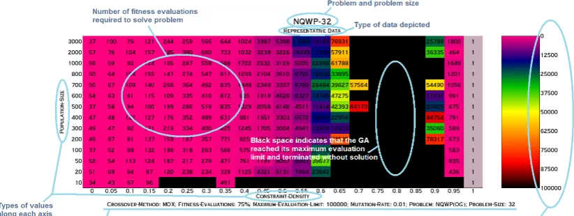
1.6 Visual Representation of Data
[image:21.612.99.510.393.548.2]In this thesis, data is most often represented in a chart with colored backgrounds to aid in the visual representation of information. This depiction style allows for a larger amount of data to share a physical space in a clearer manner than, for example, a graph with many lines and data points which may become cumbersome to read, especially when data lies near each other. Figure 1.6.1 describes explanation of notation, data representation, and where to nd pertinent information.
Chapter 2
Techniques
2.1 Crossover Methods
The following crossover techniques are utilized in this research and described in this chapter:
cycle crossover (CX)
order crossover (OX)
partially-mapped crossover (PMX)
merging crossover (MOX)
signature representations (SX)
1-point
2-point
uniform
hybrid of CX/OX/PMX/MOX (HX)
approaches and SX has been selected because of its similarities to standard crossover techniques of non-permutation-based strings. A hybrid technique was examined to gauge any potential benets of maintaining a variety of dierent crossover methods.
2.1.1 Cycle Crossover (CX)
Given permutations (zero-indexed) A and B of length n, children A0 and B0 are
created by the following algorithm[4]:
1) Assign A0 ←A,B0 ←B
2) Randomly selecticurrent such that 0≤icurrent < n, assigni0 ←icurrent
3) Mark index icurrent for crossover
4) Select inext such that A[inext] =B[icurrent]
5) Assign icurrent ←inext
6) Repeat steps 3 through 5 until icurrent =i0
7) Exchange values ofA0 and B0 on marked indexes
The purpose of the cycle found in steps 2 through 6 is to ensure that an equal set of values is to be exchanged between both permutations and that these values are to be exchanged such that no other parts of the permutation are altered in the crossover process. It can therefore be said that CX is a crossover technique that aims to be successful by preserving positions of values.
swapped, as well as when the cycle spans the entirety of the permutations (a cycle length of n) as that results in all values being swapped, in essence merely relabeling
each child in lieu of exchanging any values.
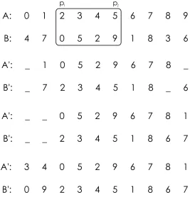
Figure 2.1.1 depicts an example of the CX crossover process.
Figure 2.1.1: Example of CX algorithm
2.1.2 Order Crossover (OX)
Given permutations (zero-indexed) A and B of length n, children A0 and B0 are
created by the following algorithm [2]:
1) Assign A0 ←A,B0 ←B
2) Randomly selectp1 and p2 such that 0≤p1 ≤p2 < n
3) For each index i such that p1 ≤i≤p2, swap A0[i]and B0[i]
4) For each child A0 and B0, if a value within the swapped portion from
5) For each child A0 and B0, starting immediately after p2 (and continuing
at the beginning of the permutation if necessary) left-shift all remaining values and blanks in the permutation so that any blank spaces appear immediately beforep1 (and at the end of the permutation if necessary)
6) For each childA0 andB0, starting immediately afterp2 (and continuing at
the beginning of the permutation if necessary) ll in blanks with values not currently represented in the permutation, in order of how they originally appeared in A and B respectively
OX preserves a contiguous section of a permutation in the resulting children, as shown in steps 2 and 3 above. OX then retains the order of the rest of the permutation, with respect to where those values appeared in the parent permutations. However, since this order begins after p2 in the child permutations and potentially wraps around
to the beginning of the permutation, OX does not necessarily preserve order in the truest sense. Whenp1andp2 are selected uniformly, the average size of the contiguous
crossover section will be roughly n
3 for large enough values of n. This derivation is
shown in Appendix Section A.
Figure 2.1.2: Example of OX algorithm
An additional variation of OX will be considered. This variation diers from the above algorithm in the following ways:
A) Instead of swapping a contiguous section of the permutation in steps 2 and 3, a certain number of values at individual positions are swapped
B) Instead of lling in values in the order they appeared starting after p2 as
is done in steps 4 through 6, values are lled in starting at the beginning of the permutation (i= 0)
2.1.3 Merging Crossover (MOX)
Given permutations (zero-indexed) A and B of length n, children A0 and B0 are
1) Randomly merge A and B into a list L
2) Let A0 be the permutation obtained by taking the rst instance of each
distinct value in L, preserving their order, and let B0 be the permutation
obtained by taking the second (last) such instance of each value in L,
again preserving order
Notice that MOX does not necessarily preserve the location of any elements. It does however preserve order in the sense that if value x precedes value y in both A
and B, x will also precede y in both A0 and B0[1]. More generally, it also has the
characteristic that when L is the result of relatively uniform merging (constructed
without exceptionally long contiguous sections from either parent), values that appear in the same vicinity in both parents will also appear in the same vicinity in both of the children.
Figure 2.1.3 depicts an example of the MOX process.
2.1.4 Partially-Mapped Crossover (PMX)
Given permutations (zero-indexed) A and B of length n, children A0 and B0 are
created by the following algorithm (adapted from Introduction to Genetic Algorithms by Sivanandam and Deepa [2] with the exception of step 4, which was not included in the cited text 1):
1) Assign A0 ←A,B0 ←B
2) Randomly selectp1 and p2 such that 0≤p1≤p2< n
3) For each child A0 and B0, create respective lists of mapping relationships
MA and MB, where for each index i such that p1 ≤i ≤ p2, B0[i] →A0[i]
is added to MA and A0[i]→B0[i] is added to MB
4) For each mapping list MA and MB, if there are cycles such that x → z, and z → y, replace those two such relationships with a single mapping
x→y; repeat until no such cycles exist1
5) For each index i such that p1 ≤i≤p2, swap A0[i]and B0[i]
6) For each index i such that 0 ≤ i < p1 or p2 < i <n, if the value A0[i]
begins a mapping inMA, replace it with the respective mapped value and if the value B0[i] begins a mapping in MB, replace it with its respective mapped value as well
PMX preserves a contiguous section of a permutation in the resulting children, as shown via steps 2 and 5 above. It also, in general, can potentially preserve the
1This necessary step is often omitted in various descriptions of this algorithm (including, for example, Introduction
to Genetic Algorithms by Sivanandam and Deepa [2] and a selected lecture [4]), assumably due to unintentional simplicity of examples accompanying the algorithm. Following this algorithm without such checks for cycles can (and likely will, at least eventually) result in permutations that repeat values: upon careful inspection, it should be evident that this will occur when there is at least one value xthat appears in bothAand Bin the range[p1, p2], but at
location of many of the values outside of the contiguous crossover section. Specically, any value not mapped by steps 3 and 4 above will remain unchanged in the child permutations. When values must be mapped in the child permutations as per step 6, the resulting set of values do not preserve any particular ordering from either parent. When p1 and p2 are selected uniformly, the average size of the contiguous crossover
section will be roughly n
3 for large enough values of n. This derivation is shown in
[image:29.612.175.444.288.591.2]Appendix Section A.
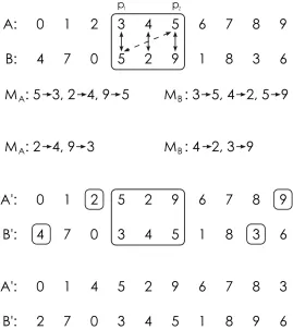
Figure 2.1.4 summarizes the PMX process.
Figure 2.1.4: Example of PMX algorithm
2.1.5 Signature Crossover (SX)
Signature crossover (SX) is a fundamentally dierent type of crossover than the previ-ously described methods. In SX, a permutation is instead represented by a signature
S of length n created such that for all i, 0 ≤ i < n, 0 ≤ S[i] < n−i. There are
n! unique signatures of length n, just as there are n! unique permutations of length
n. The use of SX allows for standard (and desirably) straightforward one-point,
two-point, and uniform crossover, among other options. A signature S can be converted
uniquely into a permutation P for tness evaluation by the following simple, O(n)
algorithm [1]:
1) For all i,0≤i < n, P[i] =i
2) For all i,0≤i < n, swap P[i] and P[i+S[i]]
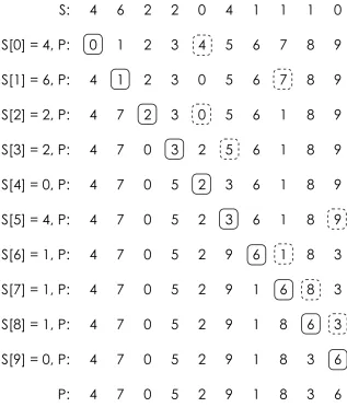
Figure 2.1.5: Example of conversion from a signature to a permutation
2.1.5.1 One-Point, Two-Point, and Uniform Crossover of Signatures
One-point crossover: Given strings (zero-indexed) A and B of length n, children A0
and B0 are created by the following algorithm:
1) Assign A0 ←A,B0 ←B
2) A crossover point p,0 < p < n, is selected uniformly, and then for all i
Two-point crossover: Given strings (zero-indexed) A and B of length n, children A0
and B0 are created by the following algorithm:
1) Assign A0 ←A,B0 ←B
2) Crossover points p1 and p2, 0< p1 < p2 < n, are selected uniformly, and
then for all i such that p1 ≤i≤p2, swap A0[i]and B0[i]
Uniform crossover: Given strings (zero-indexed)AandB of lengthn, childrenA0 and
B0 are created by following algorithm:
1) Assign A0 ←A,B0 ←B
2) For each i, 0≤i < n, with a 50% probability swap A0[i] and B0[i]
2.1.6 Hybrid Crossover (HX)
Given permutations (zero-indexed) A and B of length n, children A0 and B0 are
created by the following algorithm:
1) Randomly select crossover method OX, CX, PMX, or MOX with equal
weight.
2) A0andB0result from the randomly selected crossover method with parents
A and B as input.
2.1.7 Randomizing Individuals
2.1.8 Null Crossover
Also at times, to work within the GA code, it was convenient to establish a null crossover where for any given set of parents, the resulting set of children would be identical to the set of parents. The primary purpose of null crossover was to speci-cally alter an individual through a dierent (non-crossover) process, such as mutation.
2.1.9 Greedy Approaches
Three dierent greedy crossover substitutes/alterations were briey explored at points within this research.
2.1.9.1 GREEDY-1
The rst greedy method randomized a population of individuals as normal, and then selected the best individual at each further iteration. This individual then underwent mutation (at a rate higher than normal) until termination of the GA. By denition of this setup, if the mutated version was the new best individual, it would then be se-lected for further mutations. However, if the mutation did not improve the individual, the original would remain better and be selected again for future mutations.
2.1.9.2 GREEDY-2
2.1.9.3 GREEDY-3
The third greedy method attempted to improve the initial randomized population before employing a more traditional crossover strategy. Specically, a random pop-ulation of ten individuals was created. Then, with a standard weighted selection (described later in this chapter), an individual was selected and mutated (at a rate higher than normal). If the mutated version was superior to the original, it replaced the original individual in this version. After 200 such operations, 190 random indi-viduals were added to the population and MOX crossover took place thereafter.
2.2 Population
Across all experiments, a steady-state population was utilized [2]. This population was kept sorted by required tness evaluations at all times, mainly for purposes of selection and deselection. In practice, the sort routine need only be called once, upon initial population generation. Thereafter, insertions and removals, which each run in linear time, are sucient to maintain a sorted list.
2.3 Selection
With only few exceptions (noted shortly) exactly two parents were randomly selected, weighted toward the population's better individuals. Specically, such selection was modeled after a drawing where in a population of n individuals, the best individual
has n entries, the second best has n−1 entries, etc., and the worst individual has
For purposes of some experiments focusing on greedy approaches, the selection algo-rithm was simply to always choose the best individual as parent. In this research, such selection was always carried out as a single-parent operation so that truly only the best individual was ever selected for manipulation.
2.4 Deselection
In these experiments, only the worst individuals were deselected (or removed from the population) to make room for new children. That is, for a crossover method requiringn parents, their children always took the place of the worstn individuals in
the population. This is also the case even in instances where children may be worse performers than the individuals they replace. In other words, children always enter the population, regardless of their quality.
2.5 Mutation
For each individual (A of length n, zero-indexed) created by means of a crossover
operation, mutation was performed on it in the following manner: For each i, 0 ≤
i < n, there exists a 1% probability of randomly swapping A[i]with A[j], wherej is
a random value such that 0≤j < n.
In previous related research, mutation rate was analyzed with the PMX crossover method. Figure 2.5.1 and Figure 2.5.2 show the tness evaluations required to solve the 500-queens problem over a variety of mutation rates. Values along the y-axis
Figure 2.5.1: NQ-500: Variation of mutation rates with PMX crossover
Chapter 3
N -Queens With Poison (NQWP)
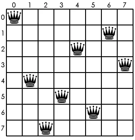
In the game of chess, the queen is a piece that may attack opponent pieces that share the same row, column, or one of the two diagonals as the queen. The goal of the
n-queens (NQ) problem is to nd one or more arrangements of n queens on an n×n
[image:37.612.192.418.416.650.2]chessboard such that no two queens are in position to attack each other [1]. For example, Figure 3.0.1 depicts one possible solution to the 8-queens problem.
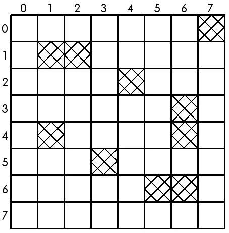
In the n-queens with poison problem, by denition, squares may be deemed as poison
and queens may not be placed on such squares. In general, any number or congura-tion of squares may be poisoned. Figure 3.0.2 depicts an8×8board with 10 poisoned
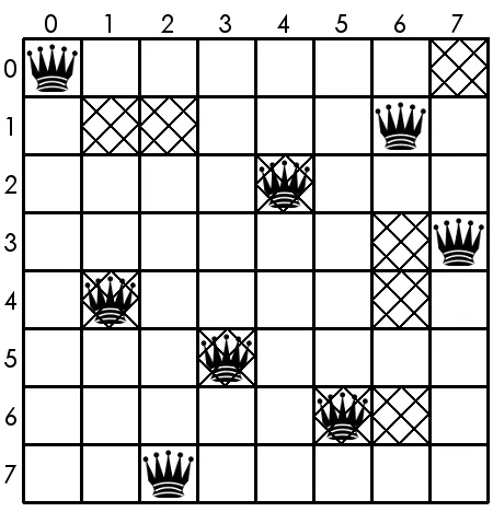
[image:38.612.192.419.218.449.2]squares, and Figure 3.0.3 shows how the solution contained in Figure 3.0.1 does not conform to the particular poisoned layout from Figure 3.0.2.
Figure 3.0.3: Solution from Figure 3.0.1 overlaid onto poisoned board from Figure 3.0.2
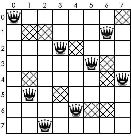
Figure 3.0.4: A solution to the 8-queens with poison problem, constrained by the board from Figure 3.0.2
3.1 Diculty
Diculty is measured by considering results after altering the percentage of poisoned squares across multiple trials of the NQWP problem for various values of n.
3.2 Problem Representation
A solution to the NQWP problem is represented by a permutation P of length n.
Specically, in the simplest representation, i is the column in which a queen is to
be placed, and P[i] contains the row. For example, the representation of the queen
as well as spaces that are susceptible to attack by previously laid queens. Fitness is measured as the percentage of queens (out of n) that can be placed legally under the
leftmost-placement guideline until a single placement fails [1].
3.3 Problem Set Creation
Instances of the NQWP problem were created through the following process:
1) Choose a constraint density csuch that 0≤c≤100 (that is, the
percent-age of spaces to be poisoned, where 0% implies no spaces are poisoned and 100% means all spaces unoccupied by queens are poisoned)
2) Choose number of queens n
3) Using a GA, solve an instance of NQWP on an n ×n board with 0%
constraint density
4) Poisonc% of the unoccupied spaces
5) Remove queens from the board
3.4 Solution Approach
Instances of the NQWP problem were solved by the following algorithm:
1) Begin with a board instance B created by the process described in
Sub-section 3.3
2) Choose a crossover methodX from those described in Section Section 2.1
3) Select the number of times r to run the GA on board B with crossover
4) Using a GA, solve for board B utilizing crossover method X a total of r
times, storing the tness evaluations from each run in array V
5) Sort V, best to worst, and output the values at the following percentiles
as arrayW: 100, 95, 90, 75, 50, 25, 10, 5, 0
3.5 Results
As can be seen in later analysis, it is important to note that such representative cannot be assumed to be representative of qualities other than what it was selected as the median of medians. For example, the representative data selected could have had the worst or worst performance at the 95th percentile or the best or near-best performance at the 25th percentile. This could further complicate potential discussion of overall winners and losers. However, by looking at medians, the data is hopefully least skewed by random factors such as unusually easy or dicult problem sets.
It is important to preface the analysis of results by noting that there in general is not an absolute clear-cut winner as far as choosing crossover methods in conjunction with population sizes. Dierences in results were often slight and very few overarching generalities could be claimed.
In the dialogue within this chapter, the term NQWP-x refers to the NQWP problem
at problem size x, that is, on an x×x board. Other more fundamental alterations
of GA parameters will also be reected in the problem name. NQWP-32 was utilized as the baseline data set.
easiest problems: ones solvable within the initial population stage. Therefore, it was not necessary x or redo such tests since it had no bearing on non-trivial data sets.
3.5.1 Diculty
3.5.1.1 Primary Results
One of the few overarching statements that can be made, NQWP-32 was most dicult at a constraint density of 0.8, with diculty tapering o at constraint densities both higher and lower than that mark. Consider Figures 3.5.1.1 through 3.5.1.1 that show 50th percentile results across all crossover methods as support.
Figure 3.5.1: CX crossover at population size 500
Figure 3.5.3: OX crossover at population size 500
Figure 3.5.4: PMX crossover at population size 400
Figure 3.5.6: SX-2POINT crossover at population size 500
Figure 3.5.7: SX-UNIFORM crossover at population size 400
This is also supported by looking at random solutions to this problem. Figure 3.5.1.1 similarly shows problem diculty centering around a constraint density of 0.8.
Additionally, even at the 95th percentile of results, no crossover exhibited any solu-tions within 100,000 tness evaluasolu-tions for a constraint density of 0.8.
3.5.1.2 Eect of Crossover Technique on Diculty
As can be seen in Figures 3.5.1.1 through 3.5.1.1, choice of crossover technique had no discernable eect on problem diculty, as problems at or near constraint densities of 0.8 were always the most dicult.
Within some individual data sets, there were occasionally instances in the lower range of constraint densities where a less constrained problem required more tness eval-uations to solve than a more constrained one. While it is possible that there may be a more fundamental underlying rationale, it is believed that it is more likely that data sets involved in such comparisons contained a higher than normal number of unusually easy or dicult data sets.
3.5.1.3 Eect of Population Size on Diculty
Figure 3.5.9: NQWP-32: MOX crossover at population size 200
Figure 3.5.10: NQWP-64: MOX crossover at population size 200
3.5.1.4 Distribution of Dicult Problems
Altogether, there were 2099 pieces of representative data from unique combinations of GA congurations for NQWP-32. At the 25th percentile mark, 803 of them ter-minated only at the 100,000 tness evaluation limit. (This general scenario shall be called limit termination.) 145 of these had population sizes of 10, which in general did not prove to yield desirable results. For other population sizes, constraint densities from 0.7 to 0.9 were represented in this 25th percentile limit-termination group. At the 5th percentile mark, and again throwing out results from population size 10, there exist limit-terminated problems at constraint densities ranging from 0.45 to 0.9.
Across all data (not just representative data) and after removing results achieved with a population size of 10, at the 50th percentile mark, limit-terminated runs can be found at constraint densities of 0.5 to 0.95. At the 5th percentile mark, limit-terminated runs begin to appear at a constraint density of 0.4. At the 0th percentile mark (showcasing the worst results), limit-terminated runs appear as early as at constraint densities of 0.1, and then appear more frequently starting at 0.3.
In summation, dicult problems do appear at constraint densities outside of those close to or equal to 0.8, however there are predictably less at constraint densities furthest away.
3.5.1.5 GA Behavior for Dicult Problems
may have on the ability of the GA to solve the problem.
3.5.1.6 Characteristics of Dicult Problems
Across problem sets created with identical constraint density, less poison in the left-most columns (or more generally, the left half of the board) and then consequently having more poison in the right portion of the board is a major factor in a data set having high diculty. As the OG algorithm lls columns in as left-to-right as possi-ble, the left columns comparatively get lled before their counterparts on the right. It should then come as no major surprise that with more poison (fewer options to place a queen) toward the end of the algorithm, the algorithm is more likely to fail having to work in this exceptionally constrained area of data.
Consider Table 3.5.1 that depicts this phenomenon for ve pairs of data sets. The rst four were selected for exhibiting vast dierences in diculty. The fth was selected for exhibiting roughly similar performance. It is clear that in each of the rst four columns, the values peak around the half-way point of the list, indicating substantially more open space on the left half than on the right.
Constr. Dens. i: 0 1 2 3 4 5 6 7 8 9 10 11 12 13 14 15 16 17 18 19 20 Data set A: 0.5 -1 -1 -3 2 7 7 9 9 10 9 10 13 16 15 24 20 28 29 30 24 21 Data set B: 0.8 2 0 2 -3 -4 -2 -2 0 3 -2 2 6 10 16 19 22 17 21 23 21 20 Data set C: 0.55 -1 -1 8 15 19 18 16 13 18 19 20 20 17 19 21 22 22 22 20 16 15 Data set D: 0.5 0 -3 2 3 10 13 3 0 3 8 4 3 8 8 15 14 19 16 15 17 15 Data set E: 0.4 3 -1 -2 0 0 -1 -4 -6 -10 -5 -4 -7 -5 -3 8 7 6 4 6 0 -1
3.5.2 Crossover Techniques
3.5.2.1 Primary Results
Overall, results tend to show that MOX, SX-2POINT, SX-UNIFORM, and PMX stand out as the best performers, perhaps in that order, although certainly not beyond argument.
Figure 3.5.12: NQWP-32: All crossovers and population sizes for 50th percentile runs at constraint density 0.25
At a constraint density of 0.5, where NQWP certainly starts to pick up more diculty, SX-1POINT has the overall best performance at population size 400. The worst individual best can be found with OX at population size 200. These results are found in Figure 3.5.13, which also shows that midrange population sizes are in general the best performers.
At an even more dicult set of problems, depicted in Figure 3.5.14, where the con-straint density is 0.6, results start to show more of a divergence in quality as far as population sizes go. While MOX is the top-performing crossover technique at a pop-ulation size of 200, more crossover techniques tend to nd their best performances at both high and low population sizes. CX's best is at population size 20, much dierent than its best for constraint density 0.5, which occurred at 800.
Figure 3.5.14: NQWP-32: All crossovers and population sizes for 50th percentile runs at constraint density 0.6
Figure 3.5.15: NQWP-32: All crossovers and population sizes for 75th percentile runs at constraint density 0.65
Constraint Density: 0.9 SX(2-POINT) 100 SX(UNIFORM) 400 SX(UNIFORM) 200 MOX 500 SX(UNIFORM) 300 CX 500 MOX 600 SX(UNIFORM) 300 MOX 600 MOX 1000 MOX 700 CX 700 SX(1-POINT) 400 MOX 700 SX(2-POINT) 300 SX(1-POINT) 800 OX 600 CX 400 SX(2-POINT) 500 PMX 400
Constraint Density: 0.7
MOX 700 MOX 1000 MOX 700 MOX 1000 MOX 600 MOX 2000 MOX 1000 MOX 1000 MOX 500 MOX 500 MOX 600 SX(2-POINT) 2000 SX(2-POINT) 2000 SX(2-POINT) 700 SX(UNIFORM) 300 MOX 700 SX(2-POINT) 2000 MOX 300 CX 20 MOX 700
Constraint Density: 0.6 SX(2-POINT) 700 MOX 300 SX(2-POINT) 500 MOX 200 SX(2-POINT) 600 MOX 300 MOX 200 MOX 600 MOX 300 MOX 200 SX(2-POINT) 700 MOX 600 MOX 500 MOX 500 MOX 400 SX(UNIFORM) 200 SX(2-POINT) 1000 SX(UNIFORM) 300 SX(2-POINT) 3000 MOX 200
Constraint Density: 0.5 SX(2-POINT) 200 SX(2-POINT) 400 SX(2-POINT) 300 MOX 100 SX(1-POINT) 600 SX(1-POINT) 400 SX(UNIFORM) 400 MOX 200 SX(2-POINT) 300 MOX 200 SX(1-POINT) 600 SX(1-POINT) 400 MOX 600 SX(UNIFORM) 300 MOX 100 SX(UNIFORM) 100 SX(1-POINT) 1000 SX(UNIFORM) 200 SX(1-POINT) 700 SX(UNIFORM) 100
Constraint Density: 0.4 SX(2-POINT) 100 SX(1-POINT) 800 PMX 50 SX(2-POINT) 100 MOX 200 MOX 50 SX(UNIFORM) 50 SX(2-POINT) 100 MOX 100 SX(1-POINT) 1000 SX(2-POINT) 700 MOX 100 SX(UNIFORM) 200 SX(2-POINT) 200 SX(UNIFORM) 50 MOX 200 SX(2-POINT) 1000 SX(2-POINT) 600 MOX 100 SX(1-POINT) 200
Constraint Density: 0.25 SX(UNIFORM) 20 SX(UNIFORM) 50 SX(1-POINT) 50 SX(UNIFORM) 20 PMX 50 PMX 100 PMX 200 SX(1-POINT) 50 MOX 100 MOX 1000 SX(UNIFORM) 20 SX(2-POINT) 50 SX(UNIFORM) 50 SX(UNIFORM) 20 SX(2-POINT) 50 MOX 50 OX 100 PMX 50 SX(1-POINT) 100 MOX 400
Table 3.5.2: Best 20 crossover method and population size congurations (sorted by 50th percentile values, across all GA runs) for selected constraint densities
stands out in easier problems.
3.5.2.2 Eect of Population Size on GA Performance
As has been alluded to in Subsections 3.5.2.1 and 3.5.1.1, performance can be quite dependant on population size. It can be seen that more moderate population sizes often attack the most dicult problems well, however both large and small popu-lation sizes have a chance to attack dicult problems well. Large popupopu-lation sizes especially may nd solutions to dicult problems, albeit at higher numbers of tness evaluations.
3.5.2.3 Crossover Variations and Substitutions
GREEDY-1 (Subsection 2.1.9.1 on page 24) was tested on NQWP-32 and undoubtedly failed. In all tests, only once did it not limit-terminate at 90th percentile (or better) results.
More success (but still worse than crossover: Figure 3.5.1.3 on page 39) was achieved with GREEDY-2 (Subsection 2.1.9.2 on page 24). First, it was run on NQWP-128, and it was determined that mutating an individual at a rate of 5% would be a solid parameter.
Figure 3.5.17: NQWP-64: GREEDY-2; 5% chance of apocalypse
GREEDY-3 (Subsection 2.1.9.3 on page 25) has more success, generally defeating its most analogous counterpart at the less constrained, easier problems, however MOX at population size 200 outperforms GREEDY-3 at the more dicult problems.
Chapter 4
Processor Scheduling (PS)
In an array of m processors that operate over a duration of n units of time, there
are m·n single-time-unit processes that can be scheduled under such a conguration.
In addition, precedence relationships can exist mandating that certain processes are to be completed before others. The PS problem is dened as scheduling these m·n
processes into a perfect schedule (that completes in n time-units) under a particular
set of precedence constraints [3].
4.1 Diculty
Diculty is measured by considering results after altering the percentage of existing precedence relations across multiple trials of the PS problem for various values of n.
4.2 Problem Representation
In the PS problem, the process schedule can be represented by a permutation P of
lengthm·n, where a process inP at indexican be said to begin at timeimodmand
on processor i divn. For OG tness evaluation purposes, the permutation contains
percentage processes (out of m ·n) that can be scheduled legally under the
rst-available-slot guideline until a single attempt fails.
4.3 Problem Set Creation
Instances of the PS problem will be created under the following guidelines:
1) Choose a constraint density csuch that 0≤c≤100 (that is, the
percent-age of precedence relations to include, where 0% implies no precedence relations and 100% means that every process requires every previously scheduled process as precedence relations)
2) Choose time n, along with number of processors m;m = 4 was primarily
utilized throughout this research
3) Create solutionSto be overlaid with the precedence relations graph, where
for each i,0≤i < m·n, S[i] =i;this is automatically a valid solution as
all numbered process labels are essentially arbitrary
4) Add c% of the possible precedence relations
5) Remove the processes from the schedule
4.4 Solution Approach
Instances of the PS problem will be solved by the following algorithm:
1) Begin with precedence relation setQ created by the process described in
Subsection 4.3
3) Select the number of timesr to run the GA on precedence relation set Q
with crossover method X
4) Using a GA, solve for precedence relation setQutilizing crossover method
X a total ofrtimes, storing the tness evaluations from each run in array
V
4a) There exists the opportunity to topologically sort individuals prior to tness evaluation to increase their quality (and thereby ideally reducing the number of tness evaluations necessary to reach a solution)
5) Sort V, best to worst, and output the values at the following percentiles
as arrayW: 100, 95, 90, 75, 50, 25, 10, 5, 0
4.4.1 Topological Sorting
4.4.1.1 Full Sort
Algorithm 4.1 Full Topological Sort for Processor Scheduling
For precedence relation setQand a (zero-indexed) individualAof lengthn, create listA0as follows:
1) Move each orphan process in A to the end of A0 maintaining relative position fromA
(rst orphan process inA appears before all other orphan processes inA0, etc.); assign kto be the number of orphan processes (the orphan processes are stored inA0[n−k−1]
throughA0[n−1])
2) For eachi,0≤i < n−k, nd the rst occurrence of a process inAwith an in-degree of
zero (that is, a process that does not require another process to complete before it can begin); call itpi
3) AssignA0[i]pi
4) Remove all precedence relations fromQthat begin withpi
5) Removepi fromA
6) Repeat steps 2-6 untilAis empty
7) (Permanently) assignA←A0
4.4.1.2 Rough Sort
Algorithm 4.2 Rough Topological Sort for Processor Scheduling
For precedence relation setQand a (zero-indexed) individualAof lengthn, create listA0as follows:
1) Move each orphan process in A to the end of A0 maintaining relative position fromA
(rst orphan process inA appears before all other orphan processes inA0, etc.); assign kto be the number of orphan processes (the orphan processes are stored inA0[n−k−1]
throughA0[n−1])
2) Assigni0
3) For j = 0, 0 ≤ j < n, nd the rst unmarked occurrence of a process in A with an
in-degree of zero or one; call itpi
4) AssignA0[i]pi
5) Remove all precedence relations fromQthat begin withpi
6) Markpi in A
7) Increasej by 1
4.4.1.3 Partially Random Sort
Algorithm 4.3 Partially Random Sort for Processor Scheduling For an individualA:
1) With 10% probability, return the results of the full sort algorithm described in Subsection 4.1
2) Otherwise, returnA unchanged
4.5 Results
The generalities described for NQWP results in Section 3.5 on page 33 are applicable here as well to preface data.
Additionally, unless stated otherwise, the rough sort was utilized as the baseline sort for PS data.
4.5.1 Diculty
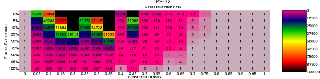
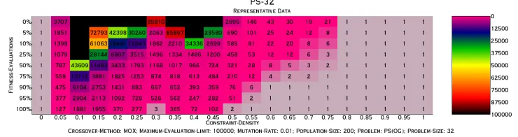
4.5.1.1 Primary Results
Figure 4.5.1: PS-32: All crossovers at population size 800; 50th percentile data
Figure 4.5.2: PS-32: All crossovers at population size 800; 10th percentile data
Figure 4.5.4: PS-32: All crossovers at population size 500; 10th percentile data
Figure 4.5.5: PS-32: All crossovers at population size 200; 50th percentile data
Figure 4.5.6: PS-32: All crossovers at population size 200; 10th percentile data
lending more credence to suggesting 0.2 is overall, perhaps the more dicult problem constraint density in general.
Constraint Density:: 0.05 0.1 0.15 0.2 0.25 0.3 0.35 0.4 0.45 0.5 0.55 0.6 Limit-Terminations 1 34 60 81 95 71 34 28 10 5 0 3
Table 4.5.1: Number of limit-terminations at 50th percentile results per constraint density across all PS-32 data
4.5.1.2 Eect of Crossover Technique on Diculty
As can be seen in the previous gures, choice of crossover technique had a mild, but noticeable eect on problem diculty, though problems at or near constraint densities of 0.2 were still generally the most dicult. Table 4.5.1.2 shows that only with MOX was the most dicult constraint density exactly 0.2. Each other crossover method exhibited most dicult behavior (at least in terms of frequency of limit-terminated run) at 0.15 or 0.25.
Const. Density: 0.05 0.1 0.15 0.2 0.25 0.3 0.35 0.4 0.45 0.5 0.55 0.6
CX 0 0 2 3 8 5 3 1 2 2 0 0
MOX 1 5 9 21 16 15 4 6 2 1 0 1
OX 0 11 16 14 8 6 3 2 0 0 0 0
PMX 0 0 4 9 12 5 5 2 2 1 0 0
SX-1POINT 0 4 13 12 11 11 9 4 2 0 0 1
SX-2POINT 0 2 6 11 16 13 9 5 1 0 0 0
SX-UNIFORM 0 2 5 4 12 11 2 1 2 1 0 1
RANDOM 0 5 6 3 3 2 3 0 0 0 0 0
Table 4.5.2: PS-32: Number of limit-terminated runs at 50th percentile across all data
4.5.1.3 Eect of Problem Size on Diculty
Figure 4.5.7: PS-64: MOX at population size 200
Figure 4.5.8: PS-128: MOX at population size 200
4.5.1.4 Distribution of Dicult Problems
As can bee seen in Table 4.5.1.2 on the previous page, dicult problems appear across a wide range of constraint densities, from 0.05 to 0.6.
4.5.1.5 GA Behavior for Dicult Problems
better-case scenarios. These cases exhibit the important eect that quality initial random conditions may have on the ability of the GA to solve the problem.
4.5.1.6 Eect of Sorting Algorithm on Diculty
[image:68.612.52.562.500.626.2]Dierent sorting algorithms do have mild eects on what constrait densities are most dicult. With CX at population size 50, fully sorted, the most dicult problems are at constraint density 0.35, as seen in Figure 4.5.1.6. While there is also great diculty at 0.35 for the rough sort implementation, depicted in Figure 4.5.1.6, there is also roughly equal diculty at lower constraint densities.
Figure 4.5.9: PS-32: Full sort, CX at population size 50
Figure 4.5.10: PS-32: Rough sort, CX at population size 50
nds the most dicult problems at constraint density 0.3, while the roughly sorted counterpart (Figure 4.5.1.6) has the most diculty at 0.1.
Figure 4.5.11: PS-32: Full sort, MOX at population size 200
Figure 4.5.12: PS-32: Rough sort, MOX at population size 200
As sorting is a major variation of tness calculation, it should be no major surprise that altering the sort may change where problems are the most dicult.
4.5.1.7 Eect of Processor Count on Diculty
While a processor count of 4 was used throughout this research, a later analysis was done exploring the eects of utilizing other processor counts. Such experiments were done using RANDOM with the full sort.
still comparatively easy to solve, and GA performance is, overall, solid. As the pro-cessor count increases, several things occur: 1) the range of diculty shifts to lower constraint densities, 2) the diculty of these problems increases, and 3) the range at which dicult problems are seen decreases. (The only observed exception to this is PS-128 at 4 processors, a value which gives relatively easy problems. Coincidentally, this again is the the processor count at which all other research into this problem utilized.) This trend holds until the processor count is equal to half the problem size, at which point the problem is trivially easy.
[image:70.612.90.525.336.460.2] [image:70.612.57.560.528.655.2]Further analysis of such problem diculty is left for future research. (See Section 5.2 on page 77).
Figure 4.5.13: PS-32: 2 Processors
Figure 4.5.15: PS-32: 8 Processors
Figure 4.5.16: PS-32: 16 Processors
Figure 4.5.18: PS-64: 8 Processors
Figure 4.5.19: PS-64: 16 Processors
Figure 4.5.21: PS-128: 2 Processors
Figure 4.5.22: PS-128: 4 Processors
Figure 4.5.24: PS-128: 16 Processors
Figure 4.5.25: PS-128: 32 Processors
4.5.2 Crossover Techniques
4.5.2.1 Primary Results
[image:75.612.104.510.272.446.2]From Subsection 4.5.1.2 on page 57 it is already evident that CX and PMX perform well. Additionally, by looking pairwise at Figures4.5.2.1 through 4.5.2.1, which depict performance at dicult constraint densities (0.15 through 0.3), their success is further evident, as well as SX-UNIFORM's.
Figure 4.5.28: PS-32: 5th percentile data; constraint density 0.15
Figure 4.5.30: PS-32: 5th percentile data; constraint density 0.2
Figure 4.5.32: PS-32: 5th percentile data; constraint density 0.25
Figure 4.5.34: PS-32: 5th percentile data; constraint density 0.3
4.5.2.2 Eect of Population Size on GA Performance
Constraint Density: 0.1 SX(UNIFORM) 50 MOX 600 PMX 300 PMX 100 SX(2-POINT) 100 MOX 100 SX(2-POINT) 100 SX(1-POINT) 500 MOX 400 OX 20 MOX 300 SX(1-POINT) 300 SX(UNIFORM) 200 CX 100 SX(1-POINT) 200 PMX 800 SX(1-POINT) 200 PMX 400 MOX 700 CX 50
Constraint Density: 0.15
OX 700 PMX 500 CX 200 CX 300 PMX 50 PMX 200 CX 200 SX(UNIFORM) 100 PMX 500 PMX 500 PMX 300 MOX 300 SX(UNIFORM) 400 SX(1-POINT) 600 CX 400 MOX 100 OX 200 PMX 100 MOX 400 SX(UNIFORM) 100
Constraint Density: 0.2
MOX 20 MOX 600 PMX 100 PMX 100 MOX 800 CX 50 SX(1-POINT) 50 PMX 20 SX(2-POINT) 100 PMX 600 MOX 200 PMX 200 PMX 700 MOX 300 CX 300 PMX 200 SX(2-POINT) 400 MOX 200 MIX 200 SX(2-POINT) 100 Constraint Density: 0.25
MOX 50 CX 20 SX(2-POINT) 20 PMX 20 PMX 50 MOX 50 OX 200 OX 20 SX(2-POINT) 400 MOX 500 PMX 400 SX(UNIFORM) 800 CX 200 MOX 500 PMX 200 MOX 200 CX 400 SX(2-POINT) 200 CX 300 SX(1-POINT) 20
Constraint Density: 0.3
MOX 100 SX(1-POINT) 50 PMX 50 OX 800 PMX 50 PMX 50 MOX 300 SX(UNIFORM) 20 SX(UNIFORM) 20 SX(UNIFORM) 50 SX(UNIFORM) 200 PMX 100 MOX 200 CX 200 OX 200 CX 100 MOX 50 OX 100 SX(UNIFORM) 50 PMX 20
Constraint Density: 0.35
OX 600 MOX 20 MOX 100 CX 100 PMX 50 PMX 50 PMX 50 CX 100 SX(2-POINT) 20 CX 20 PMX 20 PMX 700 OX 50 SX(2-POINT) 50 MOX 400 PMX 500 MOX 200 MOX 200 MOX 300 SX(1-POINT) 50
4.5.2.3 Eect of Sorting Algorithm on GA Performance
The eect of presorting PS input is profound, and the benet of a full sort exceeds the overhead required to implement such sort, at least within the methods explored in this research. Compare the results from Figures 4.5.2.3 to 4.5.2.3 against the primary results of Subsection 4.5.1.1 on page 54. In all cases, the fully sorted data severely outperforms the roughly sorted primary data.
Figure 4.5.35: PS-32: Full sort, CX at population size 10
Figure 4.5.37: PS-32: Full sort, MOX at population size 200
Figure 4.5.38: PS-32: Full sort, RANDOM search
It is also of immediate note that the RANDOM search outperforms the genetic al-gorithm when operating on fully sorted data, at least for the ranges of parameters tested. This is not necessarily a result of the GA being an inappropriate methodology as much as it shows how immensely powerful the sort is. Especially given the extent to which this sort would inevitably reorder the input, it remains a potential area of future research (see Subsection 5.2 on page 77) to determine if may be exploitable characteristics of fully sorted data that would still be amenable to a GA approach.
to even though roughly sorted input.
Figure 4.5.39: PS-32: MOX-200; Unsorted input at 50th percentile of quality
Data that utilized the partially random sort described in Subsection 4.4.1.3 on page 54 did have a considerable eect as can be seen in Figure 4.5.2.3, and did also notably outperform the roughly sorted data seen previously in Figure 4.5.1.3 on page 58.
Figure 4.5.40: PS-128: Partially random sort, MOX at population size 200
Chapter 5
Conclusion
5.1 Implications of Research
In addition to the results highlighted in each section, there are several cumulative conclusions to be made from this research.
Determining winners and losers, especially in terms of crossover method and population size, cannot always be clear-cut.
Investigation of constraint density denitively showed exact values or narrow ranges at which problems are most often dicult. However, dicult problems can still appear across wide ranges of parameters. Likewise there is not always an obvious set of baseline parameters that will result in dicult problems.
5.2 Future Work
5.2.1 Additional In-Depth Research
There are several avenues upon which futher related research could be pursued:
Testing other GA parameters or options, such as selection method, population representation, or more work with mutation rate
Implementing a crossover strategy or customized sort that directly attempts to reduce the diculty of NQWP problems or attacks dicult problems in a pointed manner
Analysis of particular qualities of dicult PS problems, and to better understand how and why particular processor counts so greatly aects where problems are dicult
Determining if there exist any ways to improve GA performance of fully sorted PS data
How results compare to non-OG or non-permutation based approaches to the same problems
Consider a more graph-theoretical approach for NQWP and then determine if any graph theory can be exploited to better solve problems
5.2.2 Additional Problems
There are many other problems along the same vein as NQWP and PS that could be examined in a similar fashion, as well as variations on NQWP and PS. Some of these possibilities are listed as follows.
5.2.2.1 Graph Coloring
A k-partite graph is a graph that can be broken into k subgraphs, where vertices
within each subgraph are unconnected by edges. For example, a tripartite (3-partite) graph can be broken into three such subgraphs. Further, a complete k-partite graph is one where each vertex in the aforementioned subgraphs is connected by edges to all vertices outside of its respective subgraph. Again using the complete tripartite graph as an example, the notation Kr,s,t is often used to represent its topography, where
r, s, and t specify the number of vertices in each subgraph [5]. Because tripartite
graphs can be broken down in this way, they may be colored using as few as three colors (such that no two vertices of the same color are connected by any edge), a point that can be extended for any positive value of k. For this problem, k-coloring
will be attempted on graphs that are subsets of complete k-partite graphs of the form
Kn, n, ..., n
| {z }
k
.
5.2.2.2 Classroom Seating
In a class ofnstudents to be assigned seats in one row ofndesks (or a matrix ofm×n
as pairs of students and nding a seating arrangement where such pairings do not occur within a conict radius of k desks of each other.
5.2.2.3 Variations on N -Queens With Poison
Apply the same principal to packing knights onto a poisoned board, or devising other pieces which may be even more dicult to place than queens, etc.
5.2.2.4 Variations on Processor Scheduling
Appendix A
Derivation of Average OX/PMX Crossover
Sec-tion Size
In selecting p1 and p2 uniformly over n, there aren choices for both p1 and p2 and to
assume without loss of generality that p1 ≤p2, it suces for work with the crossover
techniques to swap p1 and p2 if p1 > p2. The following chart shows the crossover
section sizes for each value of p1 and p2.
p1
p2
0 1 2 · · · n−2 n−1
0 1 2 3 · · · n−1 n
1 2 1 2 · · · n−2 n−1
2 3 2 1 · · · n−3 n−2
... ... ... ... ... ... ...
n−2 n−1 n−2 n−3 · · · 1 2
n−1 n n−1 n−2 · · · 2 1
Table A.0.1: Length of crossover section sizes in OX/PMX for values ofp1andp2
The average crossover section size will be computed by adding all of the individual crossover section sizes and then dividing that value by the total number of crossover sections. It is immediately clear that there are n2 (not necessarily unique) crossover
sections. There are n sections of size 1, 2(n−1)sections of size 2, 2(n−2) sections