Finding the one-loop soliton solution of the short-pulse equation by means of the homotopy analysis method

Finding the one-loop soliton solution of the

short-pulse equation by means of the

homotopy analysis method

E.J. Parkes

, S. Abbasbandy

∗

a

Department of Mathematics, University of Strathclyde, Glasgow G1 1XH, UK

b_{Department of Mathematics, Imam Khomeini International University, Ghazvin,}

34149-16818, Iran

Abstract

The homotopy analysis method is applied to the short-pulse equation in order to find an analytic approximation to the known exact solitary upright-loop solution. It is demonstrated that the approximate solution agrees well with the exact solution. This provides further evidence that the homotopy analysis method is a powerful tool for finding excellent approximations to nonlinear solitary waves.

Key words: Short-pulse equation; Homotopy analysis method; Solitary-wave solution; Series solution

1 Introduction

The solution of nonlinear problems by analytic techniques is often rather difficult. Recently, a powerful analytic method for nonlinear problems, the so-called homo-topy analysis method (HAM), has been developed by Liao [1]. The HAM has been applied successfully to many nonlinear problems in engineering and science, such as applications in heat transfer [2], solving the generalized Hirota–Satsuma coupled KdV equation [3], in heat radiation [4], finding solitary-wave solutions for the fifth-order KdV equation [5], finding the solutions of generalized Benjamin-Bona-Mahony equation [6], finding the root of nonlinear equations [7], finding the solitary-wave solutions for the Fitzhugh–Nagumo equation [8], boundary-layer flows over an im-permeable stretched plate [9], unsteady boundary-layer flows over a stretching flat

∗ _{Corresponding author.}

plate [10], exponentially decaying boundary layers [11], a nonlinear model of com-bined convective and radiative cooling of a spherical body [12], and many other problems (see [13–26], for example).

The short-pulse equation (SPE), namely

uxt =u+ 1 6(u

3

)xx, (1.1)

models the propagation of ultra-short pulses in silica optical fibers [27]. It has been shown that the short-pulse equation has a Lax pair that is of the Wadati-Konno-Ichikawa type [28,29]. Because of this result, it is not surprising that the SPE has a loop-soliton solution. This solution was found in [30,31] together with several other forms of solution.

The aim of this paper is to apply the HAM to the SPE in order to find an analytic approximation to the solitary upright-loop solution which was given in exact form by Parkes [31].

In Section 2 we give the exact solution for the solitary upright-loop solution. In Section 3 we formulate the HAM for finding an approximate analytic solution for the one-loop soliton wave. A brief conclusion is given in Section 4.

2 Exact solitary upright-loop solution

The SPE has several families of periodic travelling-wave solutions that may be expressed in terms of Jacobian elliptic functions with nonlinearity parameter m [31]. In the limit m _→ 1, a single upright or inverted loop-soliton is obtained [31, Section 3.2]. Here we discuss the upright-loop solution.

In order to seek travelling-wave solutions of (1.1) we assume that u(x, t) := U(η), where η:=x+ct−x0, and cand x0 are constants. In this case (1.1) becomes

cUηη =U+ 1 6(U

3

)ηη. (2.1)

It is found that the solitary upright-loop solution is such that U is an implicit function of η. This solution may be given in parametric form by

U = 2√csechτ , η =√c(2 tanhτ ₋τ), (2.2)

where c >0, and the parameter τ is defined by

2√cdη dτ :=U

2

3 The HAM for the upright-loop solitary wave

The loop solitary-wave solution to (2.1) forU as a function ofη is multi-valued. An approximation to this solution cannot be found directly by the HAM. In order to proceed, we need to change the independent variable to τ so that the solitary-wave solution is an smooth-hump wave for U as a function of τ. Hence we use (2.3) in (2.1) to obtain

2c Uτ τ +U(U

2

−2c) = 0. (3.1)

It is convenient to introduce a new dependent variablew(τ) defined by

u(x, t) =U(τ) :=a w(τ), (3.2)

where a is the amplitude, and w(τ) is a solitary smooth-hump wave of unit ampli-tude such that w(0) = 1, w′

(0) = 0, w _→0 as _|τ_{| → ∞}, and w(τ) =w(₋τ). Here, the prime denotes denotes differentiation with respect toτ. Substitution ofU given by (3.2) into Eq. (3.1) gives

2c w′′

+w(a2w2₋2c) = 0. (3.3)

Due to the assumed symmetry of the solitary wave, in the HAM we consider w(τ) only for τ _≥ 0. Hence the appropriate boundary conditions on w for use in the HAM are

w(0) = 1, w′

(0) = 0, w(+_∞) = 0. (3.4)

The aim is to use the HAM to find analytic approximations to w(τ) and a. Then η(τ) can be found by integrating (2.3) to obtain

η(τ) = a 2

2√c

Z τ

0 w2

(˜τ)d˜τ₋√c τ. (3.5)

From w(τ) and η(τ) we can find an approximation to the solitary loop wave given by w as an implicit function of η. The aim is to show that this approximation and the approximation to a are in good agreement with the known exact results. For simplicity, from here on we set c= 1.

According to Eq. (3.3) and the boundary conditions (3.4), the solitary-wave solution can be expressed in the form

w(τ) = +∞

X

m=1 dme

−mτ_{, (3.6)}

where the dm (m = 1,2, . . .) are coefficients to be determined. According to the rule of solution expression denoted by (3.6) and the boundary conditions (3.4), it is natural to choose

w0(τ) = 2e −τ

−e−2τ

as the initial approximation to w(τ).

We define an auxiliary linear operator L by

L[φ(τ;p)] = ∂ 2

∂τ2 −1

!

φ(τ;p), (3.8)

with the property

L[C1e

−τ_+C

2eτ] = 0, (3.9)

whereC1 andC2 are constants. This choice ofL is motivated by (3.6) and the later requirement that (3.16) should contain only one non-zero constant, namely C1.

From (3.3) we define a nonlinear operator

N[φ(τ;p), A(p)] := 2 ∂ 2

φ ∂τ2

!

+φA2(p)φ2−2, (3.10)

and then construct the homotopy

H[φ(τ;p), A(p)] = (1₋p)_L[φ(τ;p)₋w0(τ)]−¯hpN[φ(τ;p), A(p)], (3.11)

where ¯his a nonzero auxiliary parameter. SettingH[φ(τ;p), A(p)] = 0, we have the zero-order deformation equation

(1₋p)_L[φ(τ;p)₋w0(τ)] = ¯hpN[φ(τ;p), A(p)], (3.12)

subject to the boundary conditions

φ(0;p) = 1, ∂φ(τ;p) ∂τ

_τ=0 = 0, φ(+∞;p) = 0, (3.13)

where p_∈[0,1] is an embedding parameter. When the parameterp increases from 0 to 1, the solution φ(τ;p) varies from w0(τ) to w(τ), and A(p) varies from a0 to a, where a0 is the initial value of the wave amplitude. If this continuous variation is smooth enough, the Maclaurin’s series with respect to p can be constructed for φ(τ;p) and A(p), and further, if these two series are convergent atp= 1, we have

w(τ) =w0(τ) + +∞

X

m=1

wm(τ), a=a0+ +∞

X

m=1 am,

where

wm(τ) = 1 m!

∂m_φ(τ;p) ∂pm p=0

, am = 1 m!

∂m_A(p) ∂pm p=0 .

For brevity, we define the vectors

−

Differentiating Eqs. (3.12) and (3.13)m times with respect top, then settingp= 0, and finally dividing bym! , we obtain themth-order deformation equation

L[wm(τ)−χmwm−1(τ)] = ¯hRm(−→wm−1,−→am−1), (m= 1,2,3, . . .) (3.14)

subject to the boundary conditions

wm(0) = 0, w ′

m(0) = 0, wm(∞) = 0, (3.15)

where Rm is defined as

Rm = 2w ′′′ m−1+

m−1

X

n=0





m−n−1

X

j=0

(ajam−n−j−1)

n

X

i=0 wn−i

i

X

l=0

wlwi−l

!

−2w_m−1.

The general solution of Eq. (3.14) is

wm(τ) = ˆwm(τ) +C1e

−τ _+C

2eτ, (3.16)

where C1 and C2 are constants and ˆwm(τ) is a particular solution of Eq. (3.14). Using (3.6), we haveC2 = 0. The unknowns C1 and am−1 are governed by

ˆ

wm(0) +C1 = 0, wˆ ′

m(0)−C1 = 0.

Thus, the unknown am−1 is obtained by solving the linear algebraic equation

ˆ

wm(0) + ˆw ′

m(0) = 0,

and thereafter C1 is given by

C1 =−wˆm(0). (3.17)

In this way, we derive wm(τ) and am−1 for m = 1,2,3, . . ., successively. At the Mth-order approximation, we have the analytic solution of Eq. (3.3), namely

w(τ)_≈WM(τ) = M

X

m=0

wm(τ), a≈AM = M

X

m=0

am. (3.18)

The auxiliary parameter ¯h can be employed to adjust the convergence region of the series (3.18) in the homotopy analysis solution. By means of the so-called ¯ h-curve, it is straightforward to choose an appropriate range for ¯h which ensures the convergence of the solution series. As pointed out by Liao [1], the appropriate region for ¯h is a horizontal line segment.

Our solution series contain the auxiliary parameter ¯h. We can choose an appropriate value of ¯h to ensure that the two solution series converge. We can investigate the influence of ¯h on the convergence ofa by plotting the curve of aversus ¯h, as shown in Fig. 1. Clearly, a_≈2 which agrees with the expected value 2√c with c= 1.

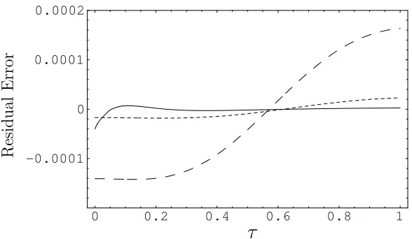
instance, our analytic solution converges, as shown by the residual error in Fig. 2. The series solution for the amplitude is convergent, and the corresponding series for w(τ) and the approximation for the upright loop U(η) are also convergent. For instance, when ¯h = −0.6, our analytic solution converges, as shown in Fig. 3 and Fig. 4.

-1.4 -1.2 -1 -0.8 -0.6 -0.4 -0.2 0 1.99

2 2.01 2.02 2.03 2.04 2.05

a

¯

h

Fig. 1: The curves of the wave amplitude a versus ¯h for the 10th-order approximation.

0 0.2 0.4 0.6 0.8 1

-0.0001 0 0.0001 0.0002

R

es

id

u

al

E

rr

or

τ

Fig. 2: The residual error for Eq. (3.3) for the 10th-order approximation. Solid curve: ¯h =₋0.7; dotted curve: ¯h=₋0.6; dashed curve: ¯h=₋0.5.

-3 -2 -1 0 1 2 3 0

0.2 0.4 0.6 0.8 1

w

τ

Fig. 3: The analytic approximation forw(τ) when ¯h =₋0.6 and the exact solution w(τ) = sech(τ). Solid curve: exact solution; symbols: 10th-order approximation.

-1 -0.5 0 0.5 1

0 0.5 1 1.5 2

U

η

Fig. 4: The analytic approximation forU(η) when ¯h =₋0.6 and the exact solution (2.2). Solid curve: exact solution; symbols: 10th-order approximation.

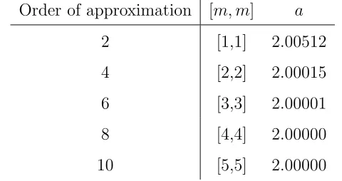
Table 1: Results for [m, m] Homotopy-Pad´e approach

Order of approximation [m, m] a

2 [1,1] 2.00512

4 [2,2] 2.00015

6 [3,3] 2.00001

8 [4,4] 2.00000

4 Conclusions

We have applied the homotopy analysis method (HAM) to the short-pulse equation (1.1) to obtain an analytic approximation to the known upright-loop solitary-wave solution as given in [31]. The HAM gives excellent agreement with the known so-lution. The HAM provides us with a convenient way to control the convergence of approximation series; this is a fundamental qualitative difference between the HAM and other methods for finding approximate solutions. The example in this paper gives further confirmation of the power of the HAM to solve complicated nonlinear problems.

References

[1] Liao SJ. Beyond perturbation: introduction to the homotopy analysis method. Boca Raton: Chapman & Hall/CRC Press; 2003.

[2] Abbasbandy S. The application of homotopy analysis method to nonlinear equations arising in heat transfer. Phys Lett A 2006;360:109–113.

[3] Abbasbandy S. The application of homotopy analysis method to solve a generalized Hirota–Satsuma coupled KdV equation. Phys Lett A 2007;361:478–483.

[4] Abbasbandy S. Homotopy analysis method for heat radiation equations. Int Commun Heat Mass Transf 2007;34:380–387.

[5] Abbasbandy S, Samadian Zakaria F. Soliton solutions for the fifth-order KdV equation with the homotopy analysis method. Nonlinear Dynam 2008;51:83–87.

[6] Abbasbandy S. Homotopy analysis method for generalized Benjamin-Bona-Mahony equation. Z Angew Math Phys (ZAMP), In Press.

[7] Abbasbandy S, Tan Y, Liao SJ. Newton-homotopy analysis method for nonlinear equations. Appl Math Comput 2007;188:1794–1800.

[8] Abbasbandy S. Soliton solutions for the Fitzhugh–Nagumo equation with the homotopy analysis method. Appl Math Model (in press),

doi:10.1016/j.apm.2007.09.019

[9] Liao SJ. A new branch of solutions of boundary-layer flows over an impermeable stretched plate. Int J Heat Mass Transfer 2005;48:2529–2539.

[10] Liao SJ. Series solutions of unsteady boundary-layer flows over a stretching flat plate. Stud Appl Math 2006;117:239–264.

[12] Liao SJ, Su J, Chwang AT. Series solutions for a nonlinear model of combined convective and radiative cooling of a spherical body. Int J Heat Mass Transfer 2006;49:2437–2445.

[13] Tan Y, Xu H, Liao SJ. Explicit series solution of travelling waves with a front of Fisher equation. Chaos, Solitons & Fractals 2007;31:462–472.

[14] Wu W, Liao SJ. Solving solitary waves with discontinuity by means of the homotopy analysis method. Chaos, Solitons & Fractals 2005;26:177–185.

[15] Sajid M, Siddiqui AM, Hayat T. Wire coating analysis using MHD Oldroyd 8-constant fluid. Internat J Engrg Sci 2007;45: 381–392.

[16] Hayat T, Sajid M. Homotopy analysis of MHD boundary layer flow of an upper-convected Maxwell fluid. Internat J Engrg Sci 2007;45: 393–401.

[17] Liao SJ, Cheung K. Homotopy analysis of nonlinear progressive waves in deep water. J Eng Math 2003;45:105–116.

[18] Sajid M, Hayat T, Asghar S. On the analytic solution of the steady flow of a fourth grade fluid. Phys Lett A 2006;355:18–26.

[19] Tan Y, Abbasbandy S. Homotopy analysis method for quadratic Riccati differential equation. Commun Nonlinear Sci Numer Simul 2008;13:539–546.

[20] Wang C. Analytic solutions for a liquid film on an unsteady stretching surface. Heat Mass Transfer 2006;42:759–766.

[21] Abbasbandy S, Parkes EJ. Solitary smooth-hump solutions of the Camassa–Holm equation by means of the homotopy analysis method. Chaos, Solitons & Fractals 2008;36:581–591.

[22] Hayat T, Abbas Z, Sajid M. On the Analytic Solution of Magnetohydrodynamic Flow of a Second Grade Fluid Over a Shrinking Sheet, ASME J Appl Mech 2007;74:1165– 1171.

[23] Hayat T, Sajid M, Ayub M. A note on series solution for generalized Couette flow. Commun Nonlinear Sci Numer Simul 2007;12:1481–1487.

[24] Hayat T, Ahmed N, Sajid M, Asghar S. On the MHD flow of a second grade fluid in a porous channel. Comput Math Appl 2007;54:407–414.

[25] Hayat T, Javed T, Sajid M. Analytic solution for rotating flow and heat transfer analysis of a third-grade fluid. Acta Mech 2007;191: 219–229.

[26] Sajid M, Hayat T. Non-similar series solution for boundary layer flow of a third-order fluid over a stretching sheet. Appl Math Comput 2007;189:1576–1585.

[27] Sch¨afer T, Wayne CE. Propagation of ultra-short optical pulses in cubic nonlinear media. Physica D 2004;196:90–105.

[28] Sakovich A, Sakovich S. The short pulse equation is integrable. J Phys Soc Jpn 2005;74:239–241.

[30] Sakovich A, Sakovich S. Solitary wave solutions of the short pulse equation. J Phys A Math Gen 2006;39:361–367.