Ceriotti, M. and Vasile, M. (2010) An ant system algorithm for automated
trajectory planning. In: World Congress on Computational Intelligence,
WCCI 2010, 2010-07-18 - 2010-07-23, Barcelona, Spain. ,
This version is available at
https://strathprints.strath.ac.uk/26350/
Strathprints is designed to allow users to access the research output of the University of Strathclyde. Unless otherwise explicitly stated on the manuscript, Copyright © and Moral Rights for the papers on this site are retained by the individual authors and/or other copyright owners. Please check the manuscript for details of any other licences that may have been applied. You may not engage in further distribution of the material for any profitmaking activities or any commercial gain. You may freely distribute both the url (https://strathprints.strath.ac.uk/) and the content of this paper for research or private study, educational, or not-for-profit purposes without prior permission or charge.
Any correspondence concerning this service should be sent to the Strathprints administrator:
The Strathprints institutional repository (https://strathprints.strath.ac.uk) is a digital archive of University of Strathclyde research outputs. It has been developed to disseminate open access research outputs, expose data about those outputs, and enable the
An Ant System Algorithm for Automated Trajectory Planning
Matteo Ceriotti, and Massimiliano Vasile,
Member, IEEE
Abstract— The paper presents an Ant System based algorithm to optimally plan multi-gravity assist trajectories. The algorithm is designed to solve planning problems in which there is a strong dependency of one decision one all the previously-made decisions. In the case of multi-gravity assist trajectories planning, the number of possible paths grows exponentially with the number of planetary encounters. The proposed algorithm avoids scanning all the possible paths and provides good results at a low computational cost. The algorithm builds the solution incrementally, according to Ant System paradigms. Unlike standard ACO, at every planetary encounter, each ant makes a decision based on the information stored in a tabu and feasible list. The approach demonstrated to be competitive, on a number of instances of a real trajectory design problem, against known GA and PSO algorithms.
I. INTRODUCTION
The complete planning of a multi-gravity assist trajectory (MGA) (i.e. the definition of an optimal sequence of plan-etary encounters and the definition of one or more locally optimal trajectories for each sequence) has been approached with two main class of techniques: two level approaches, integrated approaches.
Two-level approaches split the problem into two sub-problems which lay at two different levels: one sub-problem is to find a suitable set of sequences of planetary encounters, the other is to find at least one optimal trajectory for each sequence. Two-level approaches define the planetary sequence independently of the trajectory itself [1]. They use a simplified, low fidelity, model at the first level to quickly assess many, if not all, sequences and a more accurate model, at lower level, to optimize the trajectory. Each sequence is represented by a string of integer numbers, while the associated trajectory is represented with a string of mixed real and integer numbers defining all the characteristics of the events occurring along the trajectory (e.g. launch, deep space maneuver, arrival at a celestial body, number of revolutions around the Sun, etc.).
The main issue with two-level approaches is to assess the optimality of a given planetary sequence without an exhaus-tive search for all possible trajectories associated to that sequence. Unfortunately, finding an optimal trajectory is a very difficult global optimization problem in itself. This, combined with the fact that usually there exist a very high number of sequences for a given transfer problem, requires a considerable computational effort. The computational cost
Matteo Ceriotti is with the Advanced Space Concepts Laboratory, Depart-ment of Mechanical Engineering, University of Strathclyde, Glasgow, G1 1XJ, UK (phone: +44 141 548 5726; email: [email protected]).
Massimiliano Vasile is with the Space Advanced Research Team, De-partment of Aerospace Engineering, University of Glasgow, James Watt South Building, G12 8QQ, Glasgow, UK (phone: +44 141 3306465; email: [email protected]).
can be reduced by discarding non-promising sequences. However, if the low-fidelity model is not accurate enough, either some good sequences are discarded, or many of the retained ones can result to be not good.
As opposed to the two-level approaches, integrated ap-proaches define a mixed integer-continuous optimization problem, which tackles both the search of the sequence and the optimization of the trajectory, using a single model, at the same time [2]. This kind of problems is known in literature as a hybrid optimization problem [3], [4]. The main difficulty with integrated approaches is that a variation of even a single celestial body in the sequence corresponds to a substantially different set of trajectories. Therefore, if the solution of the hybrid optimization problem is represented with a single vector, a small variation of some of its components can lead to a huge variation of the cost function. In addition, a variation of the length of the sequence implies varying the number of legs of the trajectory, and thus the total length of the solution vector.
The automatic design of a trajectory with discrete events was recently formulated by Ross et al. as a Hybrid Optimal Control Problem [3], and a solution was proposed by Wall and Conway [5] with a two level approach based on Genetic Algorithms. In Conway’s approach an outer loop selects the sequence and an inner loop finds sets of optimal solutions. A single model is used and this partially mitigates the difficulties of two level approaches.
modified ACO does not use standard pheromone deposition and evaporation heuristics but employs tabu lists, to guide the decision of the ants at each planet (or node), and an external archive to build a stochastic model of the search space. In the literature, some ACO-derived meta-heuristics exist for the specific solution of different scheduling problems. In particular, Merkle et al. [9] proposed to apply ACO to the solution of the Resource-Constrained Project Scheduling Problem, while Blum, in his work [10], suggested the hy-bridization of Ant Colony Optimization with a probabilistic version of Beam Search for the solution of the Open Shop Scheduling problem.
Recently, some authors have hybridized ant systems with tabu search for applications such as the Job-Shop Scheduling problems [11], [12] or the data clustering problem [13]. The algorithms proposed in the literature use tabu search to improve locally the solutions or to avoid re-visiting nodes in a tree. The modified ACO algorithm in this paper, instead, employs tabu lists to discriminate between feasible and infeasible paths. In fact, because of the dependency problem, at every node, feasible and infeasible directions are undistinguishable without the memory of the past moves of the ants.
The paper is organized as follows: the MGA planning problem will be briefly introduced, then the modified ACO algorithm will be described in details with an analysis of its complexity; a discussion will follow comparing the proposed planning algorithm against standard ACO. Finally, two case studies will demonstrate the effectiveness of the proposed approach against Genetic Algorithms (GA) and Particle Swarm Optimization (PSO).
II. THEMGA PLANNINGPROBLEM
Conceptually, an MGA trajectory can be seen as a sched-uled sequence of events (e.g. launch, targeting deep space manoeuvre, swing-by, planetary capture) characterized by a set of integer variables identifying the type of event and a set of real variables identifying the time and characteristics of the event.
A trajectory model was recently proposed that transforms the above mentioned scheduled sequence of events, with the associated mixed integer-real set of variables, into a finite space of unscheduled discrete events [14]. The discrete events are: launch, deep space manoeuvre, swing-by, and planetary capture. Each event is seen as an action required to transfer the spacecraft from one celestial body to another. A complete trajectory is made of a sequence of legs connecting
nP + 1 celestial bodies [P0, P1, . . . , PnP]. The trajectory starts from P0 at time t0 with the direction of the velocity
vector after launch ϕ0 (see Ceriotti et al. [14] for more
details). The first leg goes from P0 to P1, then a number
of swing-by’s and interplanetary legs follow, until the final planetPnP. Thus, a complete trajectory withnP+ 1planets hasnP legs, andnP−1 swing-by’s.
Each transfer from a planetPi to a planetPi+1 is fully
char-acterized by five parameters mDSMi,nrev1,i,nrev2,i,fp/a,i andf1/2,i:mDSMi is the magnitude of the velocity change
(or DSM) along the transfer arc fromPi toPi+1,nrev1,i the
number of revolutions around the Sun prior to the DSM,
nrev2,i the number of revolutions around the Sun after
the DSM, fp/a,i defines where the DSM occurs (only two
positions are allowed, pericenter and apocenter of the transfer arc) andf1/2,idefines at which intersection the spacecraft is
going to meet the planet Pi+1 (only two intersections are
possible along the orbit of the planet). A complete plan is, therefore, defined assigning a value to Pi and to the
vector bi = [mDSMi, nrev1,i, nrev2,i, fp/a,i, f1/2,i]T for all
i= 0, ..., nP −1. A partial or incomplete plan is the set of
parameters sufficient to describe a solution up to transfer i. If at transferithere is no vector xi such that the spacecraft can be transferred from Pi to Pi+1 the plan is said to be
broken and the solution is said to be infeasible at transferi. The MGA planning problem can be formulated as the unconstrained minimization problem:
min
x∈Dy (1)
where y is the cost function associated to a complete plan, D is the search space and x =
[t0, ϕ0, P0,b1, P1,b1, ..., Pi,bi, ..., PnP,bnP−1]T. If each
real and integer variable in x can assume only k discrete values and j planets are available at every encounter then
k2j24k3 are the possible paths from P
1 to P2 and for
nP + 1planets the number of paths arek2Qn
P
(j24k3).
A. Solution coding
The set of parameters inxis inhomogeneous, as it is made of real, integer and binary variables. Thus, in the present implementation, the values of the departure date t0 and
the departure angle ϕ0, are assumed to be pre-assigned
and therefore the two parameters are removed from x. The rationale behind this choice is that, if an algorithm exists that is able to efficiently generate a complete plan for a given
t0, then an unidimensional search in the time domain can
be performed to find the optimal launch date. The angle
ϕ0 on the other hand is often a mission requirement [1].
Furthermore, it is assumed that the departure planet P0 is
given a priori.
Each solution representing a plan is encoded using a vector sof positive integers. The vector has2nP components. Each pair of consecutive components encodes all the parameters necessary to characterize one transfer, or segment of the plan (Fig. 1). The first element of the pair encodes the identification number of the target planet according to the following procedure: given the ordered setQP,i, containing
all the celestial bodies available at transferi, and the index if
j =s2(i−1)+1, then the target planet isqP,ij∈ QP,i, where
now igoes from1 tonP.
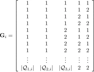
The second element of the pair is the row index of the matrix Gi containing all the possible combinations of indexes identifying the elements of the five sets:Q1,i={q1,i|q1,i∈
R}, Q2,i = {q2,i|q2,i ∈ N}, Q3,i = {q3,i|q3,i ∈ N},
Q4,i = {q4,i|q4,i ∈ {0,1}}, Q5,i = {q5,i|q5,i ∈ {0,1}}.
Fig. 1. Vector for coding a three-leg solution.
Gi=
1 1 1 1 1
1 1 1 1 2
1 1 1 2 1
1 1 1 2 2
1 1 2 1 1
1 1 2 1 2
1 1 2 2 1
1 1 2 2 2
..
. ... ... ... ...
|Q1,i| |Q2,i| |Q3,i| 2 2
(2)
where|.|denotes the cardinality of a set. Each row ofGi is a vector representing a different type of transfer. In general, the matrix has |Q1,i| · |Q2,i| · |Q3,i| · |Q4,i| · |Q5,i| rows,
which is also the number of possible different transfers for a given segment of a plan. The parameters for the jth type of transfer can be obtained as follows: mDSMi = q1,ik1,
nrev1,i = q2,ik2, nrev2,i = q3,ik3, fp/a,i = q4,ik4, f1/2,i =
q5,ik5, where k1 = Gi,j1, k2 = Gi,j2, k3 = Gi,j3, k4 =
Gi,j4,k5=Gi,j5.
III. THET-ACO ALGORITHM
The algorithm for the solution of the MGA planning problem, called T-ACO in the following, starts from organizing the search space as an acyclic oriented tree. Each branch of the tree represents a segment of the plan, while each node (or leaf) represents a different destination planet and type of transfer. A population of virtual ants are dispatched to explore the tree, searching for an optimal solution. The search runs for a given number of iterations niter,max, or
until a maximum number of objective function evaluations
neval,max has been reached. An evaluation is a call to the
trajectory model, in order to compute the objective value associated to a given solution. Algorithm 1 illustrates the main iteration loop. Each iteration consists of two steps: first, a solution generation step (lines 2 to 8), and then a solution evaluation step (line 9). In the former step, the ants incrementally compose a set of solution vectors, while the latter invokes the trajectory model to assess the feasibility and the objective value of each generated solution. Feasible solutions are stored in a feasible list while infeasible solutions are stored in a number of tabu lists.
A. The Tabu and Feasible Lists
The transfer from planet Pi to planet Pi+1 can be feasible
or infeasible, for the same set of parameters, depending on
Algorithm 1 Main T-ACO algorithm
1: Set number of ants equal tom 2: for allk= 1, ..., mdo
3: Generate planetary sequence
4: Generate types of transfers
5: if s is not discardedthen
6: S←S∪ {s}
7: end if
8: end for
9: Evaluate all solutions inS 10: Update feasible list and tabu list
11: Termination Unless niter > niter,max ∨ neval >
neval,max, GoTo Step 1
all the preceding transfers from 0 to(i−1). For this reason, when a plan contains an infeasible transfer, it is necessary to store the whole path that led to that infeasible transfer. Thus, all the parameters characterizing the partial solution up toPi
are stored in a tabu list.
In particular, if the problem involvesnP transfers, the same
number of tabu lists are used. The tabu list of transfer i
contains all the partial solutions, which are feasible up to
Pi. The tabu list is stored in a matrix (one for each transfer),
which has an arbitrary number of rows and2icolumns. The number of elements in the tabu lists can be limited, to limit the memory requirements and the search time. Once one of the tabu lists is full, the optimizer can either stop or simply start replacing the older elements.
Dual to the list of tabu partial solutions, the feasible list stores all the solutions, which are completely feasible, i.e. reach the destination planet. The feasible list is a matrix with an arbitrary number of rows and 2nP columns. Since each
solution contained in the feasible list is complete, then it is possible to associate an objective value to each one of them. As for the tabu list, the length of the feasible list can be limited to save memory. In this case, when the list is full, the optimization can either stop or simply the feasible solutions with the worst objective value can be replaced.
B. Solution generation
The tree is simultaneously explored, from root to leaves, by
by picking from the listQP,i. The selection depends on the
discrete probability distribution vector dP,i (one for every
transfer), which contains the probability associated to each body in QP,i. Every time an ant is at transferi, the
proba-bility distribution vector is reset to dP,i= [1,1, . . . ,1]T, i.e.
all the planets have equal probability to be chosen, and the ant sweeps the entire listQP,isubstituting the identification
number of each element inQP,i into theith odd component
of the solution vectors. Then, the feasible list is searched, for all solutions that have a (partial) planetary sequence which matches the one in s. Say that the jth element of Q
P,i is
added to s, and the resulting partial sequence matches the partial sequence of the lth solution in the feasible lists, then the probabilitydP,ijassociated to thejth element ofQP,iis
increased as follows:
dP,ij←dP,ij+
1 yl
wplanet (3)
The amount of probability which is added depends on the objective value yl of the matching solution in the feasible
list, and on the weight wplanet. Thus, the probability of
choosing thejthplanet increases according to the number of times it generates a promising sequence (leading to a feasible solution), to the value of the feasible solution itself, and to the parameter wplanet.
This mechanism (summarized in Algorithm 2) is analogous to the pheromone deposition of standard ACO and aims at driving the search of the ants toward good planetary sequences. In fact, those planets which generate (partial) sequences that appear either frequently in the feasible list, or rarely, but with a low objective function are selected with a higher probability. On the other hand, the probability of selecting other planets remains positive, such that one or more ants can probabilistically choose a planet that generates an undiscovered sequence. Note that, if the feasible list is empty, then all the planets have the same probability to be selected. The parameter wplanet controls the learning rate
of the ants. A low value of wplanet will make the term
wplanet/yl small, and thus the probability distribution will
not change much, even if the solution appears repeatedly in the feasible list, or with low values ofy. Thus, a relatively low value of wplanet will favor a global exploration of the
search space, while a high value of wplanet will greatly
increase the probability of choosing a planet which led to a feasible sequence.
Algorithm 3 assigns a value to the index j, given the (non-normalized) probability distribution vector dP,i [7]. The procedure iterates for all the transfers. At the end, all the odd entries of the solutionscontain a target planet and the planetary sequence is complete.
2) Type of Transfer Generation: Once an ant has filled in the odd components of a solutions, it proceeds assigning values to the even components. Similarly to the planet sequence generation, for each transfer all the available types of transfer are assigned, one at the time, to the solution s. A vector s for which a value is assigned to both the odd and even components up to leg i represents a partial solution. For
Algorithm 2 Planetary sequence generator
1: for alli= 1, ..., nP do
2: setd←[1,1, . . . ,1]T
3: for alltarget body j available at transferi do
4: s(1+2(i−1))←j
5: for allsolutionsl, in the feasible list, that match
sdo
6: dP,ij←dP,ij+y1lwplanet
7: end for
8: end for
9: s(1+2(i−1))←SelectProbabilityDistribution(dP,i)
10: end for
Algorithm 3Function j←SelectProbabilityDistribution(d)
1: r←U(0,1)P
jdj
2: j←1 3: p←d1
4: whilep < r do
5: j←j+ 1 6: p←p+dj
7: end while
each new partial solution, the tabu list is first checked. If the partial solution appears in the tabu list, then it means that this solution will be infeasible, regardless of the way it is completed. The probability of the type of transfer associated to that partial solution is set to zero, to avoid future selection of that path. If the partial solutions does not appear in the tabu list, the feasible list is searched for any matching partial solution. For every match found, the probability distribution for that type of transfer is modified as follows:
dt,ij ←dt,ij+
1 yl
wtype (4)
where the vector dt,i contains the probability distribution associated to the rows of the matrixGi, and the weightwtype is introduced with analogous meaning towplanet. In fact, the
higher the coefficient, the higher the chances that solutions similar to the feasible ones are generated. Conversely, a low value of wtype will favor the selection of sequences
with a different type of transfer, thus increasing the random exploration of the whole solution space. If, at a given legi, all possible transfer types correspond to partial solutions in the tabu list, the vector of probability distribution di will be full of zeros. As a consequence, the solution sis discarded, and the ant can stop its exploration of the tree.
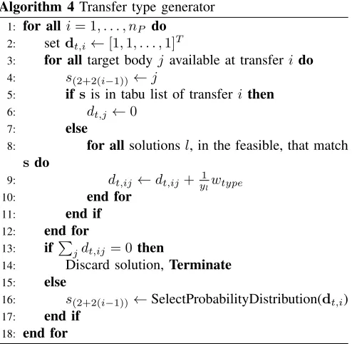
At the end of the solution generation step, the solution sis either discarded or completed. Once all the ants complete their exploration, the result is a number of solutions (less than or equal to the number of antsm) to be evaluated. The procedure is summarized in Algorithm 4.
C. Solution Evaluation
Algorithm 4 Transfer type generator
1: for alli= 1, . . . , nP do
2: setdt,i ←[1,1, . . . ,1]T
3: for alltarget bodyj available at transferi do
4: s(2+2(i−1)) ←j
5: if sis in tabu list of transferithen
6: dt,j←0
7: else
8: for allsolutionsl, in the feasible, that match
sdo
9: dt,ij ←dt,ij+y1lwtype
10: end for
11: end if
12: end for
13: ifP
jdt,ij = 0then
14: Discard solution,Terminate
15: else
16: s(2+2(i−1)) ←SelectProbabilityDistribution(dt,i)
17: end if
18: end for
If a solution is infeasible at transfer number i its objective value is set to y= +∞and the solution is stored in theith tabu list. If a solution is feasible, instead, it is stored in the feasible list.
D. Algorithm Complexity Analysis
The number of possible alternative solutions to the planning problem depends on the number of available celestial bodies for each planetary encounter, and on the values mDSM,i,
nrev1,i, nrev2,i, fp/a,i, f1/2,i. In particular if one assumes
that, at each planetary encounter, ki possible planets are
available, while mDSM,i, nrev1,i and nrev2,i can take ki
discrete values each, then the total number of possible transfers (or plans), fornP planetary encounters, isQn
P
i 4ki3.
If the values ki are equal for each encounter then the total
number of plans is 4nPk3nP
which is exponential with the number of encounters.
The ants avoid exploring the entire tree of possible plans but need to save the feasible solutions and the tabu solu-tions respectively in the feasible and tabu lists. Thus, the algorithmic complexity is mainly driven by the access to the feasible and tabu lists. In the worst case scenario all plans, but one, turn out to be infeasible only at the last planetary encounter, therefore the tabu list of the last encounter grows exponentially. If all the plans were feasible, then the tabu lists would be empty, and the feasible list would contain only the solutions explored by the ants at each repetition of the algorithm. Givenmants andniteriterations of the algorithm,
the length of the feasible list would grow asniterm.
However, on average, a number of plans will be infeasible afternp−iplanetary encounters, others afternp−i+ 1,np−
i+ 2,...,np−1. All the infeasible plans at encounter np−i
are terminated and therefore are not included in the tabu list of any subsequent encounter. If the fraction of tabu transfers at each planetary encounter isp∈[0 1], then at the first one,
only4k3(1−p)transfers will survive to the next encounter.
The tabu list of the next encounter will be 16k6(1−p)p
long and at the very last encounter the tabu list will be
4nPk3nP(1−p)nP−1plong. This would be the algorithmic
complexity if the ants were exploring all possible feasible transfers. In actuality, the number of elements in the tabu lists will grow with the number of explored plans per iteration which is at most equal to the number of ants, therefore, for
m ants the maximum length of a tabu list at encounteri is
mi(1−p)i−1p.
E. Comparison with Standard ACO
The way in which the ants generate the solutions in T-ACO (or tours, to use T-ACO nomenclature) is similar to what happens in the TSP with standard ACO [7]: each ant, independently of the others, generates a tour by adding nodes (or cities) one at a time. Each node is chosen probabilistically among a set of available nodes: for the TSP, the available nodes are the cities which have not been visited in the current tour; for the MGA, nodes are all the possible pairs of bodies and types of transfers. For both frameworks, the probability is distributed over all the possible choices, and then a selection is made, according to the probability distribution. In the case of standard ACO, the probability associated to each city depends on a heuristic function and on the pheromone deposited along the edge connecting the current city to the next city. In the case of T-ACO, instead, the generation of a solution is done in two steps: the definition of the planetary sequence and the definition of the type of transfer. Both steps use the same approach: the probability is computed by taking into account the objective value of all feasible solutions which share the same partial solution. In addition, tabu lists are checked to avoid generating solutions which are known to be infeasible. Tabu lists have no equivalent in standard ACO, because for the TSP all the solutions are feasible. Furthermore, the ants are allowed to visit the same tour more than once, as this will reinforce the amount of pheromone along the whole tour.
The evaluation step can be seen as the analogous of the pheromone deposition in standard ACO, with one difference. In T-ACO the pheromone cannot be assigned to individual transfers: this is due to the fact that each transfer (identified by its pair of integers) has no intrinsic value within the plan, if disconnected from the previous transfers. In fact, the actual value of a transfer depends on its initial conditions, which are in turn depend on all the previous transfers.
To explain this idea, we make reference to Fig. 2 and Fig. 3(a): the former shows a typical instance of the TSP. In this problem, the distance between each pair of cities is fixed, and the relative distances ofncities can be stored in a
[image:6.595.53.300.57.298.2]Fig. 2. A five-node instance of the TSP, with two possible solutions, identified by continuous and dashed arrows.
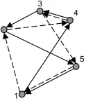
This is not true in the MGA case. Fig. 3(a) is a representation of a simple instance of the MGA problem: it has 3 transfers, 2 set of parameters for each transfer, 2 planets for the swing-bys, and 1 target planet. Each node represents a possible planet in combination with a type of transfer. The pairs of numbers next to each node in Fig. 3(a) are the two integers identifying the transfer in the solution vector (see section II-A). A solution is generated by selecting one node for each transfer, thus generating a tour which connects the starting node to one of the final nodes. The figure represents two possible solutions to the MGA problem: [1, 1, 2, 1, 1, 1] (continuous line) and [2, 2, 2, 1, 1, 1] (dashed line). These two solutions share the same parameters for the last transfer: [1, 1]. This means that they reach the same target planet with the same type of transfer. Because of the dependency of each transfer on the initial conditions, it is not possible to state that the last transfer has the same value for both solutions: in fact, the two trajectories can be consistently different, and lead to different final conditions and objective functions. For this reason, it makes no sense, for example, to assign a value to the set of parameters [1, 1] of transfer 3 in Fig. 3(a); while it is possible to assign a value to the edge 3-4 in Fig. 2.
[image:7.595.73.275.468.612.2](a) (b)
Fig. 3. Two different representations of the MGA problem: a) TSP-like representation of a three-leg MGA problem with two solutions, identified by continuous and dashed arrows; b) expanded tree representation of the same MGA problem.
A different representation of the continuous-line solution in Fig. 3(a) is the one shown in Fig. 3(b) in which every branch of the tree depends on the previous ones. In Fig. 3(b), it is clear that the set of parameters [1, 1] for transfer 3 belongs to two different solutions.
IV. CASESTUDIES
The proposed optimization method was applied to three instances of the design of transfers to planet Jupiter. Many reference solutions, computed with STOUR, can be found in a work by Petropoulos et al. [1].
For all tests t0 and ϕ0 are pre-assigned and correspond to
the launch date and direction of a known optimal solution. The tests, in fact, aim at assessing the ability of T-ACO to efficiently generate a complete plan given a set of initial conditions. T-ACO was tested against two implementation of Genetic Algorithms, the MATLAB Genetic Algorithm and Direct Search Toolbox (GATBX) [15] and NSGA-II [16], and an implementation of Particle Swarm Optimization (PSOt) [17]. Settings for the typical parameters of each one of the optimizers will be specified for each test case. Note that all the optimizers were applied to the solution of problem (1) after applying the solution coding in section II-A. For all the algorithms the parameter pop defines the size of the population. The number of generations in GA algorithms is denoted by Generations and the number of iteration in PSOt by the parameter iter. For the specific meaning of the parameters StallGenLimit, pcross bin, pmut bin, iiw and fiw, please refer respectively to [15], [16], and [17].
Due to the stochastic nature of the heuristics used in the tests, all the algorithms were run for 200 times. Two perfor-mance indexes are used to compare T-ACO against the other global optimizers: the percentage of times an algorithm finds feasible solutions and the percentage of times the objective valueyof the feasible solutions isy <y˜+ǫ, or success rate. The valuey˜is the best known objective function for a given problem. According to the theory developed in [18] 200 runs give an error in the determination for the exact success rate of less than 5% with 95% confidence.
Some preliminary tests showed that the best performance of T-ACO is achieved if the algorithm is run in 2 steps, using different sets of parameters. In particular, in the first step, the weights wplanet, wtype are set to 0. Remembering Eq.
(3) and Eq. (4), this choice translates into an initial pure random search. In fact, the solutions in the feasible list do not alter the probability distribution. On the other hand, the probability of tabu partial solutions is still set to zero to avoid their re-exploration. In the second step, weights are set to non-null values, to intensify the exploration around known feasible solutions. The values of wplanet, wtype are chosen
such that:
wplanet, wtype= ¯w·yˆ (5)
where yˆ is the expected minimum value for the objective function. In this way, by choosing for example w¯ = 1, a 1 is added to the probability of a given element every time a matching solution with objectiveyˆappears in the feasible list. The value of the added probability is higher if the objective value of the matching feasible solution is lower than yˆ. All the tests were run on an Intelr Pentium-4, 3 GHz
A. Transfers to Jupiter via Venus,Earth and Mars
In this mission, the spacecraft departs from Earth to reach a scientific orbit around Jupiter with minimum relative arrival velocity v∞. We considered the launch date t0 =
3308.5MJD2000 to reproduce one of the results in [1]. T-ACO was applied to the design of three different instances of this problem: A) Earth-Jupiter transfer via gravity assist of Venus and Earth only, with maximum three swing-by’s and no resonant transfers, B) Earth-Jupiter transfer via gravity assist of Venus and Earth only, with maximum four swing-by’s and no resonant transfers, C)Earth-Jupiter transfer via gravity assist of Venus, Earth and Mars, with resonant transfers. The launch angle was set to ϕ0 = 3.3744radians
after some preliminary investigations. The range of values for all the planet-to-planet transfers, except for the last one, are reported in Table I for each one of the instances of the problem.
TABLE I
SETTINGS FOR THE FOUR INSTANCES OF THE PROBLEM.
ID N. QP Q1 Q2 Q3 Q4 Q5
GA’s (km/s)
A 3 {Earth, {-0.05, -0.02, Ø Ø {0,1} {0,1}
Venus, -.01, 0 .01, Jupiter} 0.02, 0.05}
B 4 {Earth, {-0.05, -0.02, Ø Ø {0,1} {0,1}
Venus, -.01,0,.01, Jupiter} 0.02, 0.05}
C 4 {Earth, {-0.05, -0.02, Ø {0,1} {0,1} {0,1}
Venus, -.01,0,0.01, Mars, 0.02,0.05}
Jupiter}
The last planet-to-planet transfer is always to Jupiter and fol-lowing sets of values apply:QP ={Jupiter},Q1 = Ø,Q2=
Ø,Q3= Ø,Q4= Ø,Q5= Ø.
With the sets of values presented above, the average time for the evaluation of one plan is 0.01 s. Depending on the instance the number of plans (feasible and infeasible) is: 592704 for instance A, 49787136 for instance B, and 2.5176e+009 for instance C. Thus, a systematic scan of all the possibilities would require respectively: 1.65 hours, 13.83 hours, 6993.3 hours.
Since the transfer is towards the outer planets of the so-lar system the total time of flight tends to be very long. Therefore, the objective function is the weighted sum of the total time of flight T and the v∞: y = v∞+σT,the weight σ = 1/1000 km/s/d. The total time of flight was limited to a maximum of 100 years. This bound may seem to be too high, since a realistic time span of a transfer to Jupiter is around 6 years. However, the model considers all the solutions longer than the specified threshold on the time of flight to be infeasible, and the optimizer saves them in the tabu lists. Therefore, limiting the time of flight to lower values would over-constrain the search for optimal solutions. Better results are obtained by allowing long solutions to be returned as feasible, and introducing their duration into the objective function.
TABLE II
SETTINGS OFGATBX, NSGA-IIANDPSO.
GATBX NSGA-II PSOt Par. Value Par. Value Par. Value
StallGenLimit +Inf pcross bin 0.5 iiw 0.9 pmut bin 0.5 fiw 0.4
gen. 23 gen. 23 iter 110 pop 200 pop 200 pop 40
T-ACO was run for 600 iterations with both weights equal to zero, and for 600 with the weights wplanet, wtype= 20ˆy
km/s andyˆ= 3 km/s. These values provide good results on the same optimization problem and correspond to about 4300 function evaluations for instance A and 4800 for instance B. However, because of the normalization in Eq. (5), the weight values appear to have general validity, and can be applied to other transfer problems, as was shown in previous works [14]. With these settings, a run of T-ACO takes, on average, 60s for instance A, 150 s for instance B, 250 s for instance C. This is considerably faster than the exhaustive scan of the solution space.
NSGA-II, PSOt and GATBX were run at first for the same number of function evaluations of T-ACO and then for a number of functions valuations comparable to the number of calls to tabu and feasible lists. In fact, in T-ACO, the ants call the lists rather than calling the model to evaluate the feasibility or optimality of a particular path. If the cost of running the model is higher than accessing the lists then T-ACO is more competitive. At present the access to the list is not optimal and is coded in MATLAB. Therefore, it is not competitive against fully compiled codes like NSGA-II. Furthermore, T-ACO often finds solutions that are feasible up to the last transfer, while the other algorithms evaluate many infeasible solutions. Infeasible solutions are computationally faster than feasible ones because the trajectory model exits at some intermediate leg.
The settings used for GATBX and NSGA-II are reported in Table II. The comparative results for the two sets of runs are shown in Table III. The results in brackets are for the same number of function evaluations of T-ACO. It can be seen that T-ACO found feasible solutions in 100% of the the runs for all the instances. GATBX instead finds only 17% of feasible solutions for instance A, 55% for instance B and 74.5% for instance C. NSGA-II behaves better with results comparable to T-ACO if the number of function evaluations is substantially extended to match the run time. If the number of function evaluations is maintained constant, instead, the performance drops significantly. Note also that the quality of the solutions found by T-ACO is better than for the other algorithms. PSOt performs poorly in all cases, which might be due to a bad setting of the algorithm.
TABLE III
PERFORMANCES OFT-ACO, GATBX, NSGA-IIANDPSOT ON THE3 INSTANCES OF THEEARTH-JUPITER TRANSFER PROBLEM.
Optimizer Average best value % runs<y˜+ǫ % feasible runs (km/s)
Instance A y˜+ǫ=11.5km/s
T-ACO 11.47 64.5% 100%
GATBX 11.50(11.49) 16%(12%) 17.5%(24%) NSGA-II 11.51(11.54) 26% (7%) 91%(46%) PSOt 11.54(11.57) 1%(0.5%) 5%(4%)
Instance B y˜+ǫ=12.0km/s
T-ACO 14.62 14.5% 100%
GATBX 15.67(15.27) 6.5%(4%) 55.5%(41%) NSGA-II 15.10(17.1) 16.5%(7%) 100%(85.5%) PSOt 16.53(17.03) 0%(0%) 19.5%(7.5%)
Instance C y˜+ǫ=14.0km/s
T-ACO 13.63 90% 100%
GATBX 14.81 19% 74.5%
NSGA-II 13.19 (16.68) 99.5%(6%) 100% (98.5%) PSOt 13.77(15.91) 52% (12%) 75% (66%)
TABLE IV
SOME INTERESTING SOLUTIONS FOUND BYT-ACO.
Reference v0=3.68 T=6.3 v∞= 5.3
[km/s] [y] [km/s]
Sequence V E E J
mDSM [km/s] 0.0 0.0 0.0 0
nrev1 0 0 0 0
nrev2 0 0 0 0
T-ACO v0=3.31 T=6.72 v∞= 5.62
[km/s] [y] [km/s]
Sequence V E E J
mDSM [km/s] 0.05 0.02 -0.01 0
nrev1 0 0 0 0
nrev2 0 0 0 0
fp/a 0 1 1 0
f1/2 0 1 0 1
T-ACO v0=3.33 T=7.8 v∞= 5.51
[km/s] [y] [km/s]
Sequence V E E E J
mDSM [km/s] 0.05 0.0 -0.02 -0.05 0
nrev1 0 0 0 0 0
nrev2 0 0 0 0 0
fp/a 0 1 1 1 0
f1/2 0 0 0 1 1
ACKNOWLEDGEMENTS
This work was done when Matteo Ceriotti was a PhD student in the Space Advanced Research Team of the University of Glasgow.
V. CONCLUSIONS
The paper introduced a modified Ant Colony Optimization algorithm, called T-ACO, for planning problems in which the value associated to the outcome of an action depends on the history of all the preceding actions. T-ACO was applied to the solution of the MGA planning problem in which, the number of possible paths increases exponentially with the number of planetary encounters.
T-ACO operates an effective search thank to the use of an external archive of feasible and tabu solutions. The algorithm
demonstrated the remarkable ability to find good solutions with a very high success rate, performing better than known implementations of Genetic Algorithms and PSO.
As T-ACO requires very little information on the MGA problem under investigation, it represents a valuable tool for the complete automatic design of future space missions. Furthermore, the proposed use of tabu lists appears to be an effective solution for those planning problems in which the value of one segment of the plan depends on all the preceding segments. Future work aims at a more efficient handling of the lists, which is currently the major bottleneck of the T-ACO implementation.
REFERENCES
[1] A. E. Petropoulos, J. M. Longuski, and E. P. Bonfiglio, “Trajectories to jupiter via gravity assists from Venus, Earth, and Mars,”Journal of Spacecraft and Rockets, vol. 37, no. 6, pp. 776–783, 2000. [2] M. Vasile and P. D. Pascale, “Preliminary design of multiple
gravity-assist trajectories,”Journal of Spacecraft and Rockets, vol. 43, no. 4, pp. 794–805, 2006.
[3] I. M. Ross and C. N. D’Souza, “Hybrid optimal control framework for mission planning,”Journal of Guidance, Control, and Dynamics, vol. 28, no. 4, pp. 686–697, 2005.
[4] O. V. Stryk and M. Glocker, “Decomposition of mixed-integer optimal control problems using branch and bound and sparse direct colloca-tion,” inADPM 2000 The 4th International Conference on Automation of Mixed Processes: Hybrid Dynamic Systems, Dortmund, Germany, 2000.
[5] B. J. Wall and B. A. Conway, “Genetic algorithms applied to the solution of hybrid optimal control problems in astrodynamics,”Journal of Global Optimization archive, vol. 44, pp. 493–508, 2009. [6] A. E. Rizzoli, R. Montemanni, E. Lucibello, and L. Gambardella,
“Ant colony optimization for real-world vehicle routing problems. from theory to applications,”Swarm Intelligence, vol. 1, pp. 135–151, 2007. [7] M. Dorigo and T. St¨utzle, Ant colony optimization. Cambridge,
Massachusetts: The MIT Press, 2004.
[8] M. Dorigo and L. M. Gambardella, “Ant colony system: A cooperative learning approach to the traveling salesman problem,”IEEE Transac-tions on Evolutionary Computation, vol. 1, no. 1, pp. 53–66, 1997. [9] D. Merkle, M. Middendorf, and H. Schmeck, “Ant colony optimization
for resource-constrained project scheduling,”IEEE Transactions on Evolutionary Computation, vol. 6, no. 4, pp. 333–346, 2002. [10] C. Blum, “Beam-ACO hybridizing ant colony optimization with beam
search: An application to open shop scheduling,” Computers and Operations Research, vol. 32, no. 6, pp. 1565–1591, 2005.
[11] V. P. Eswaramurthy and A. Tamilarasi, “Hybridization of ant colony optimization strategies in tabu search for solving job shop scheduling problems,” International Journal of Information and Management Sciences, vol. 20, pp. 173–189, 2009.
[12] K.-L. Huang and C.-J. Liao, “Ant colony optimization combined with taboo search for the job shop scheduling problem,”Computers and Operations Research, vol. 35, pp. 1030–1046, 2008.
[13] A. N. Sinha, N. Das, and G. Sahoo, “Ant colony based hybrid optimization for data clustering,”Kybernetes, vol. 36, no. 2, pp. 175– 191, 2007.
[14] M. Ceriotti and M. Vasile, “Automatic mga trajectory planning with a modified ant colony optimization algorithm,” inProceedings of 21st International Symposium on Space Flight Dynamics, Toulouse, France, 2009.
[15] D. E. Goldberg, Genetic algorithms in search, optimization and machine learning. Boston, MA, USA: Addison Wesley, 1989. [16] K. Deb, S. Agrawal, A. Pratap, and T. Meyarivan, “A fast elitist
non-dominated sorting genetic algorithm for multi-objective optimization: NSGA-II,” inProceedings of 6th International Conference on Parallel Problem Solving from Nature, PPSN VI, Paris, France, 2000. [17] B. Birge, “Psot, a particle swarm optimization toolbox for matlab,” in
Proceedings of the IEEE Swarm Intelligence Symposium, 2003. [18] M. Vasile, E. Minisci, and M. Locatelli, “A dynamical system