The inverse problem for some special spectral data
V. O. Vakhnenkoa,∗, E. J. Parkesb
aInstitute of Geophysics, National Academy of Sciences of Ukraine, 01054 Ky¨ıv, Ukraine bDepartment of Mathematics & Statistics, University of Strathclyde, Glasgow G1 1XH,
UK
Abstract
In this paper the spectral problem of third order for the inverse scattering transform (IST) method is solved. For the discrete part of the spectral data, the two-multiple poles are taken into account. The line spectrum of contin-uum states for the IST method is examined as well. The suggested spectrum approximates in first order the step-function. The scope for the suggested spectral data is demonstrated through the analysis of the Vakhnenko-Parkes equation that allows new solutions to be obtained. The account of the time-dependence is different from the standard procedure.
Keywords: inverse problem, spectral data, poles of second order, line spectrum of continuum states
PACS: 00.30.Lk, 02.30.Jr, 05.45.Yv
1. Introduction
The inverse scattering transform (IST) method is one of the fundamental methods for solving various nonlinear evolution equations. The method en-ables one to solve the initial value problem for a nonlinear evolution equation. Moreover, it provides a proof of the complete integrability of the equation. The essence of the application of the IST is as follows. The equation of inter-est for study is written as the compatibility condition for two linear equations (the Lax pair). Then the initial condition is mapped into the scattering data. It is important that the spectrum always retains constant values. The time
∗Corresponding author
Email addresses: [email protected](V. O. Vakhnenko),
evolution of scattering data is simple and linear. From a knowledge of scat-tering data evolution, the solution is reconstructed. Hence, for this method the direct spectral problem and the inverse spectral problem are considered. The latter consists of reconstructing the solution of the nonlinear equation from the spectral data (§2). In the general case it is necessary to analyze both the discrete part and the continuum part of the spectral data. It is well-known that the discrete part is associated with soliton solutions, while the continuum part of the spectral data is related to the periodical solutions. For the spectrum of bound states, we take into account the two-multiple poles (§3), while for continuum states, a special form of the spectral data is considered (§4). The spectrum of continuum states is taken as a line spec-trum that in first order approximates the step-function (§4). The problem of reconstructing the solution from the spectral data is considered in §5 and
§6. The solution for discrete spectral data with two-multiple poles is taken in §7.
2. The spectral problem
The inverse problem forN×N spectral equations has been considered by Caudrey [1–3] and Kaup [4]. Following the method described by Caudrey [1], the spectral equation for many evolution equations can be written
∂
∂Xψ= [A(ζ) +B(X, ζ)]·ψ. (2.1)
For the sake of convenience, we study the third-order form of the spectral equation (2.1). The third-order spectral equation is associated with a Boussi-nesq equation [1–6], a higher order KdV equation [4, 7], a model equation for shallow water waves [8, 9], and the Vakhnenko–Parkes equation (VPE) [10–14]. The VPE arises from another nonlinear integrable equation, named the Vakhnenko equation (VE) [15, 16]
∂ ∂x
(
∂ ∂t+u
∂ ∂x
)
u+u= 0, (2.2)
after an appropriate change of variables [10, 11, 17, 18].
It is interesting to note that equation (2.2) follows as a particular limit of the following generalized Korteweg-de Vries equation
∂ ∂x
(
∂u ∂t +u
∂u ∂x −β
∂3u ∂x3
)
derived by Ostrovsky [19] to model small-amplitude long waves in a rotating fluid (γu is induced by the Coriolis force) of finite depth. Subsequently, equation (2.2) was known by different names in the literature, such as the Ostrovsky-Hunter equation, the short-wave equation, the reduced Ostrovsky equation and the Ostrovsky-Vakhnenko equation depending on the physical context in which it is studied.
Using the VPE [10–14]
WXXT + (1 +WT)WX = 0 (2.3)
or, in equivalent form with U ≡WX,
U UXXT −UXUXT +U2UT = 0
as an example, we aim to examine both the two-multiple poles and some special forms of the spectral data for which the inverse problem can be solved.
After the Lax pair
ψXXX +WXψX −λψ= 0, (2.4)
3ψXT + (1 +WT)ψ+µψX = 0 (2.5)
for the VPE was derived in [10], in [20] the Lax pair was written in its original variables as a zero curvature condition. Moreover, in [20] Hone and Wang have shown that there is a subtle connection between the Sawada-Kotera hierarchy and the VE, between the Degasperis-Procesi equation (DPE) and the VE (see also [21]), and between the Lax pairs of the DPE and the VE.
As expected, (2.4) and (2.5) are similar to, but cannot be transformed into, the corresponding equations for the Hirota–Satsuma equation (HSE) (see Eqs. (A8a) and (A8b) in [22]). Clarkson and Mansfield [23] note that the scattering problem for the HSE is similar to that for the Boussinesq equation which has been studied comprehensively by Deift et al. [6].
The explicit soliton solution for the VPE was obtained by the IST method in [10] and by the Hirota method in [17, 18, 24] whereas, for the Cauchy problem at long-time, the IST approach was presented for a Riemann-Hilbert problem [25, 26] in original (physical) independent variables for the VE in [26]. As usual, the transformation between the solution of the VPE and the VE is in the form (2.12), (2.13) in [17].
The spectral equation (2.4) has a matrix form (2.1) with
ψ=
ψψX
ψXX
, A=
0 1 00 0 1
λ 0 0
, B=
00 00 00
The matrixAhas eigenvaluesλj(ζ) and left- and right-eigenvectors ˜vj(ζ) and
vj(ζ), respectively. These quantities are defined through a spectral parameter
λ as
λj(ζ) = ωjζ, λ3j(ζ) =λ,
vj(ζ) = λj1(ζ)
λ2j(ζ)
, v˜j(ζ) =
(
λ2
j(ζ) λj(ζ) 1 )
, (2.7)
where ωj = e2πi(j−1)/3 are the cube roots of 1 (j = 1, 2,3). Obviously the
λj(ζ) are distinct and they and ˜vj(ζ) andvj(ζ) are analytic throughout the
complex ζ-plane.
The solution of the system of the linear equations (2.1) has been ob-tained by Caudrey [1, 3] in terms of Jost functions ϕj(X, ζ) which have the asymptotic behaviour
Φj(X, ζ) := exp{−λj(ζ)X}ϕj(X, ζ)→vj(ζ) as X → −∞. (2.8)
Caudrey [1] showed how the Eq. (2.1) can be solved by expressing it as a Fredholm integral equation.
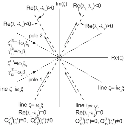
The complexζ-plane is to be divided into regions such that, in the interior of each region, the order of the numbers Re(λi(ζ)) is fixed (see Fig. 1). As we
pass from one region to another this order changes and hence, on a boundary between two regions, Re(λi(ζ)) = Re(λj(ζ)) for at least one pair i̸=j. The
residue of a simple pole can be calculated as Resϕi(X, ζi(k)) =
n ∑
j=1
j̸=i
γij(k)ϕj(X, ζi(k)). (2.9)
The quantities ζi(k) and γij(k) constitute the discrete part of the spectral data in the case of simple poles.
In contrast to the papers [1, 3] we do not restrict ourselves to simple poles. Indeed, one of the results we will prove in the next section is that the two-multiple poles can be taken into account in the discrete part of the spectral data.
Now we consider the singularities on the boundaries between regions. However, in order to simplify matters, we first make some observations. The solution of the spectral problem can be facilitated by using various symmetry properties. In view of (2.1), we need only consider the first elements of
ϕi(X, ζ) =
ϕϕi(i(X, ζX, ζ))X
ϕi(X, ζ)XX
, (2.10)
while the symmetry
ϕ1(X, ζ/ω1) = ϕ2(X, ζ/ω2) =ϕ3(X, ζ/ω3) (2.11)
means we need only considerϕ1(X, ζ). In our case, forϕ1(X, ζ), the complex
ζ-plane is divided into four regions by two lines (see Fig. 1) given by (i) ζ′ =ω2ξ, where Re(λ1(ζ)) = Re(λ2(ζ)),
(ii) ζ′ =−ω3ξ, where Re(λ1(ζ)) = Re(λ3(ζ)),
(2.12) where ξ is real. The singularity ofϕ1(X, ζ) can appear only on these
bound-aries between the regular regions on the ζ-plane and it is characterized by functions Q1j(ζ′) at each fixed j ̸= 1. We denote the limit of a quantity, as
the boundary is approached, by the superfix ± in according to the sign of Re(λ1(ζ)−λj(ζ)) (see Fig. 1).
In [1] (see Eq. (3.14) there) the jump of ϕ1(X, ζ) on the boundaries is
calculated as
ϕ+1(X, ζ)−ϕ−1(X, ζ) =
3
∑
j=2
where, from (2.12), the sum is over the lines ζ′ = ω2ξ and ζ′ =−ω3ξ given
by
(i) ζ′ =ω2ξ, with Q (1)
12(ζ′)̸= 0, Q (1)
13(ζ′)≡0,
(ii) ζ′ =−ω3ξ, with Q (2)
12(ζ′)≡0, Q (2)
13(ζ′)̸= 0.
(2.14)
The quantitiesQ1j(ζ′) along all the boundaries constitute the continuum part
of the spectral data.
Thus, for simple poles, the spectral data are [1, 3]
S ={ζ1(k), γ1(kj), Q1j(ζ′);j = 2, 3, k = 1, 2, . . . , m}. (2.15)
One of the important features which is to be noted for the IST method is as follows. After the spectral data have been obtained, we need to seek the time-evolution of the spectral data. In Refs. [10–14] it is proved that for the VPE the T-dependence is revealed as
ϕi(X, T, ζ) = exp [
−(3λi(ζ))−
1
T]ϕi(X,0, ζ),
then for spectral data (2.15)
ζj(k)(T) =ζj(k)(0), γ1(kj)(T) =γ1(kj)(0) exp
{[
−(3λj(ζ
(k) 1 )
)−1
+
(
3λ1(ζ (k) 1 )
)−1]
T
}
,
Q1j(T;ζ′) = Q1j(0;ζ′) exp {[
−(3λj(ζ′))−1+ (3λ1(ζ′))−1
]
T}.
(2.16)
The final step in the application of the IST method is to reconstruct the matrixB(X, T;ζ) and the solutionW(X, T) from the spectral dataS(2.15). Caudrey has proved that for simple poles the spectral data define Φ1(X, ζ)
uniquely in the form (see Eq. (6.20) in [1]))
Φ1(X, T;ζ) = 1−Ωd(X, T;ζ) + Ωc(X, T;ζ), (2.17)
where
Ωd(X, T;ζ)≡ K ∑
k=1 3
∑
j=2
γ1(kj)(T)exp{[λj(ζ
(k)
1 )−λ1(ζ (k) 1 )]X}
λ1(ζ (k)
1 )−λ1(ζ)
×Φ1(X, T;ωjζ1(k)),
Ωc(X, T;ζ)≡
1 2πi
∫ ∑3
j=2
Q1j(T;ζ′)
exp{[λj(ζ′)−λ1(ζ′)]X}
ζ′ −ζ
×Φ−1(X, T;ωjζ′)dζ′.
(2.19)
Equations (2.17)–(2.19) contains the spectral data, namely K simple poles with the quantitiesγ1(kj)for the bound state spectrum as well as the functions
Q1j(ζ′) given along all the boundaries of regular regions for the continuous
spectrum. The integral in (2.18) is along all the boundaries (see the dashed lines in Fig. 1). The direction of integration is taken so that the side chosen to be Re(λ1(ζ)−λj(ζ))<0 is shown by the arrows in Fig. 1 (for the lines (2.12),
ξ sweeps from−∞ to +∞).
It is necessary to note that we should carry out the integration along the lines ω2(ξ+ iε) and −ω3(ξ+ iε) with ε > 0. In this case the condition (2.8)
is satisfied. Passing to the limit ε→0 we can obtain the periodical solution which does not satisfy the condition (2.8). However, for any finite ε > 0, the restricted region on X can be determined where the solution associated with a finite ε > 0 (for which the condition (2.8) is valid) and the solution associated withε= 0 are sufficiently close to each other. In this sense, taking the integration at ε = 0, we remain within the inverse scattering theory [1], and so the condition (2.8) can be omitted. The solution obtained at ε = 0 can be extended to sufficiently large finite X. Thus, we will interpret the solution obtained at ε= 0 as the solution of the VPE (2.3) which is valid for arbitrary but finite X.
With appropriate choice of values for ζ, the left-hand side in (2.17) can be Φ1(X, T;ωjζ
(k)
1 ), or by allowing ζ to approach the boundaries from the
appropriate sides, the left-hand side can be Φ−1(X, T;ωjζ′). We acquire a set
of linear matrix/Fredholm equations in the unknowns Φ1(X, T;ωjζ1(k)) and
Φ−1(X, T;ωjζ′) [1]. The solution of this equation system enables one to define
Φ1(X, T;ζ) from (2.17).
By knowing Φ1(X, T;ζ), we can take extra information into account,
namely that the expansion of Φ1(X, T;ζ) as an asymptotic series in λ−11(ζ)
connects with W(X, T) as follows (cf. Eq. (2.7) in [4]): Φ1(X, T;ζ) = 1−
1 3λ1(ζ)
In the remaining sections we will study both the multiple poles for the discrete part of spectral data and the continuum part of the spectral data in special form. Apart from the relation (2.18), all other formulas are true for the suggested spectral data and will be used subsequently.
3. The two-multiple poles
For single poles the formula (2.18) are true. Now we take into account the two-multiple poles. Let us consider the additional equation to the spectral equation (2.4)
χXXX +WζXψX +WXχX −ζ3χ−3ζ2ψ = 0. (3.1)
Forχ=ψζ the equation (3.1) stems from (2.4) by differentiation with respect
toζ. For convenience, the spectral parameterλis written asλ=ζ3 by virtue of (2.7).
The matrix form of the system of equations (2.4) and (3.1) is as (2.1) with ψ= ψ ψX ψXX χ χX χXX
, A=
0 1 0 0 0 0 0 0 1 0 0 0
ζ3 0 0 0 0 0
0 0 0 0 1 0 0 0 0 0 0 1 3ζ2 0 0 ζ3 0 0
, B=
0 0 0 0 0 0
0 0 0 0 0 0
0 −WX 0 0 0 0
0 0 0 0 0 0
0 0 0 0 0 0
0 −WζX 0 0 −WX 0 . (3.2)
The matrixAhas three pairs of 2-multiple eigenvalues and right-eigenvectors
λj(ζ) = λj+3(ζ), λj(ζ) =ωjζ, λ3j(ζ) = λ,
vj(ζ) = 0 0 0 1
λj(ζ)
λ2
j(ζ)
=vj+3(ζ) =
0 0 0 1
λj+3(ζ)
λ2
j+3(ζ)
It is known [27] that for system (2.4), (3.1) at W = 0 to every pair of vectors
vj(ζ),vj+3(ζ) (j = 1, 2, 3), there corresponds a system of solutions
ψj =vjexp(λjX), ψj+3 = (vj +Xv2j) exp(λjX), (3.4)
where (see p. 97 in [27])
Avj =λjvj, Av2j =λjv2j+vj. (3.5)
The multiplicity of eigenvalues does not allow us to obtain the fundamen-tal system of solutions for the system (2.4), (3.1). To avoid this obstacle we introduce the equation
χXXX +WζXψX +WXχX −(ζ+ε)3χ−3(ζ+ε)2ψ = 0 (3.6)
instead of equation (3.1). The system (2.4), (3.6) in matrix form has the matrix
A=
0 1 0 0 0 0
0 0 1 0 0 0
ζ3 0 0 0 0 0
0 0 0 0 1 0
0 0 0 0 0 1
3(ζ+ε)2 0 0 (ζ+ε)3 0 0
(3.7)
with different eigenvalues and right-eigenvectors, which in the first approxi-mation O(ε) have the forms
λj(ζ) = ωjζ, λj+3(ζ) =ωj(ζ+ε),
vj(ζ) =
−ε
−ελj
−ελ2j
1
λj
λ2
j
, vj+3(ζ) =
0 0 0 1
λj+3
λ2j+3
, j = 1, 2,3. (3.8)
As ε→0 the relations (3.8) tend to (3.3). AtW = 0 the solutions of system (2.4), (3.6) are
ψj =vjexp(λjX), j = 1 . . . 6. (3.9)
In the accepted approximationO(ε), we takeψj+3 =vj+3(1+ωjεX) exp(λjX)
Since the eigenvalues (3.8) for matrixA (3.7) are different, we can state that a fundamental system of solutions for the system of the equations (2.4), (3.6) exists (here, for the sake of convenience, the variable X is omitted), namely
ϕj(λj(ζ)), j = 1 . . .6. (3.10)
According to [1, 3] we consider the Wronskian
W r = det [ϕ1(λ1), ϕ2(λ2), . . . ,ϕ6(λ6) ]. (3.11)
If the Wronskian W r is non-zero at least at one point X0, then it is proved
in [27] (see p. 132 there) to be finite and non-zero even when ζ approaches a pole.
Let ϕ1(λ1(ζ)) have poles at ζ = ζ1(k), (k = 1,2). Then (ζ −ζ (k)
1 )W r =
det
[
(ζ−ζ1(k))ϕ1(λ1), ϕ2(λ2), . . . ,ϕ6(λ6)
]
and taking the limitζ →ζ1(k) we obtain
0 = det [ Resϕ1(λ1), ϕ2(λ2), . . . ,ϕ6(λ6) ]. (3.12)
Thus the columns (vectors) are linearly dependent. The dependence on the vector ϕ4(λ4) is omitted, since it has the same poles as ϕ1(λ1) at ε→0.
As a result from (3.12), we obtain the solution of the spectral equation (2.4) for the bound state spectrum
Φ1(X;ζ) = 1− 2
∑
k=1 3
∑
j=2
[
˜
γ1(kj)exp{[λj(ζ
(k)
1 )−λ1(ζ (k) 1 )]X}
λ1(ζ (k)
1 )−λ1(ζ)
×Φ1(X;ωjζ
(k) 1 )
+˜γ1(kj+3) exp{[λj(ζ
(k)
1 +ε(k))−λ1(ζ1(k)+ε(k))]X}
λ1(ζ (k)
1 +ε(k))−λ1(ζ)
×Φ1(X;ωj(ζ
(k)
1 +ε(k)))
]
.
By expanding the functions depending on ε(k) in series within accuracy of
O(ε(k)), we rewrite the solution
Φ1(X;ζ) = 1− 2
∑
k=1 3
∑
j=2
{
γ1(kj)exp{[λj(ζ
(k)
1 )−λ1(ζ1(k))]X}
λ1(ζ (k)
1 )−λ1(ζ)
×Φ1(X;ωjζ
(k) 1 )
+ ∂
∂ζ1(k)
[
γ1(kj)+3exp{[λj(ζ
(k)
1 )−λ1(ζ (k) 1 )]X}
λ1(ζ (k)
1 )−λ1(ζ)
×Φ1(X;ωjζ
(k) 1 )
]}
,
(3.14)
where γ1(kj) = ˜γ1(jk)+ ˜γ1(kj+3) , γ1(kj+3) =ε(k)γ˜1(kj+3) . It is important to note that the solution (3.14) is independent of ε(k) now.
The relationship (3.14) formally passes into (5.1), (5.2) with appropriate change of variables. For this reason the reconstruction of the solution W
for (3.14) is similar to the problem we will consider for the special form of continuum states (5.1).
4. Special form for the continuum part of the spectral data
Now we consider the continuous spectrum of the associated eigenvalue problem (2.1), (2.6), (2.7), i.e. assume that at least some of the functions
Q1j(ζ′) are non-zero. At each fixed j ̸= 1 the functions Q1j(ζ′)
character-ize the singularity of Φ1(X, ζ). As we have shown, this singularity can
ap-pear only on boundaries between the regular regions on the ζ-plane, where the condition Re(λ1(ζ′)−λj(ζ′)) = 0 defines these boundaries [1]. For the
VPE (2.3), as we know, the complex ζ-plane is divided into four regions by two lines (2.14)
(i) ζ′ =ω2ξ, with Q(1)12(ζ′)̸= 0, Q (1)
13(ζ′)≡0,
(ii) ζ′ =−ω3ξ, with Q (2)
12(ζ′)≡0, Q (2)
13(ζ′)̸= 0,
Recently in [12–14] we have considered the singularity functions Q1j(ζ′)
on the boundaries, on which the Jost function ϕ1(X, ζ) is singular, in the form (m= 1, 2, ..., M) on the line ζ′ =ω2ξ
Q(1)12(ζ′) =−2πi
M ∑
m=1
q12(2m−1)δ(ζ′−ζ2′n−1),
Q(1)13(ζ′) =−2πi
M ∑
m=1
q13(2m−1)δ(ζ′−ζ2′n−1)≡0,
(4.1)
and on the line ζ′ =−ω3ξ
Q(2)12(ζ′) =−2πi
M ∑ m=1
q12(2m)δ(ζ′−ζ2′n)≡0,
Q(2)13(ζ′) =−2πi
M ∑ m=1
q13(2m)δ(ζ′−ζ2′n).
(4.2)
Now we extend the functional dependence for Q1j(ζ′). We focus on the
step-function as a possible singularity function
f(x) = 1
h(Θ(x)−Θ(x−h)), (4.3)
where Θ(x) is a Heavyside function. Expanding the Heavyside function Θ(x− h) into a Taylor series in the neighborhood of the point x
Θ(x−h) = Θ(x) +
∞
∑
n=1
(−1)nh
n
n!Θ
(n)(x), (4.4)
the step-function (4.3) can be rewritten in terms of the derivatives δ(n)(x) =
Θ(n+1)(x) as follows
f(x) =
∞
∑
n=1
(−1)n+1h
n−1
n! Θ
(n)(x) = ∞
∑
n=0
(−1)n h
n
(n+ 1)!δ
(n)(x)
=δ(x)−12hδ(1)(x) +. . . .
(4.5)
We restrict our consideration to only two terms of the series (4.5) for mod-elling the singularity functions Q1j(ζ′). In the limit h → 0, the functions
Q1j(ζ′) = −
2πi
h q1j(Θ(ζ
(4.1), (4.2). Therefore the singularity functions Q1j(ζ′) that we will examine
have the following forms (m = 1) on the line ζ′ =ω2ξ:
Q(1)12(ζ′) =−2πi
(
q(1)12δ(ζ′−ζ1′)− 1 2q
(1)
12h1δ(1)(ζ′−ζ1′)
)
,
Q(1)13(ζ′)≡0, i.e. q13(1) ≡0, h1 =h(1),
(4.6)
and on the line ζ′ =−ω3ξ:
Q(2)12(ζ′)≡0, i.e. q12(2) ≡0, Q(2)13(ζ′) =−2πi
(
q(2)13δ(ζ′−ζ2′)− 12q13(2)h2δ(1)(ζ′−ζ2′)
)
,
h2 =h(2).
(4.7)
Consequently, the spectral data for the continuum spectrum with special singularity functions (4.6), (4.7) are
S ={ζl′, q1(lj), hl;j = 2, 3, l = 1, 2}. (4.8)
5. The inverse spectral problem for a special continuum spectrum Let us consider the problem of reconstructing the solution W(X) from the spectral data (4.8). This will be straightforward if we can find the vec-tors Φ1(X, T;ζ). Now we study only the special form of the continuum
part of the spectral data (4.6), (4.7), while the variable Ωd(X, T;ζ) (2.18) is
considered to be identically zero. For the singularity functions (4.6), (4.7) the relationship (2.17) with (2.19) is reduced to the form (provisionally the time-dependence is not written)
Φ1(X, ζ) = 1− 2
∑
l=1 3
∑
j=2
[
q1(lj)Lj(X;ζl′, ζ)Φ1(X, ωjζl′)
+1 2q
(l) 1jhl
(
∂
∂ζ′Lj(X;ζ
′, ζ)Φ
1(X, ωjζ′) )
ζ′=ζ′l ]
,
(5.1)
where
Lj(X;ζ′, ζ)≡
exp{[λj(ζ′)−λ1(ζ′)]X}
We note once again that the relationships (3.14) and (5.1) are similar. As was proved in Refs.[12–14], the singularities appear in pairs
ζ1′ =ω2ξ1, ζ2′ =−ω3ξ1, (5.3)
where ξ1 is a real constant. Moreover
ω2q (1) 12 =q
(2)
13. (5.4)
It is evident that from (5.3)
h1 =ω2h, h2 =−ω3h,
where h is a real constant.
Here it is convenient to note that the time-evolution of the spectral data appears through (2.16) in the form
ξ1 = const, h= const, q (k)
1j (T) =q
(k)
1j (0) exp (
1 i√3
T ξ1
)
. (5.5) The equation (5.1) allows us to define the functions Φ1(X, ζ). Indeed,
differentiating this equation (5.1) with respect of ζ, and substituting the values ζ =ω2ζ1′, ζ =ω3ζ2′ in the left-hand side of these equations, we obtain
a system of four linear algebraic equations in the unknowns Φ1(X, ω2ζ1′),
Φ1(X, ω3ζ2′),
∂ ω2∂ζ
Φ1(X, ω2ζ)
ζ=ζ1′
, ∂
ω3∂ζ
Φ1(X, ω3ζ)
ζ=ζ2′
. Hence, we could take the function Φ1(X, ζ) from Eq. (5.1).
However, there is a more direct method, in which there is no need to obtain the variables Φ1(X, ω2ζ1′), Φ1(X, ω3ζ2′) explicitly. It turns out that
we need to calculate only a determinant of some matrix. This approach is similar to the method referred to in [1, 3, 10, 12–14]. It is convenient to use new variables introduced by the definition
Ψl(X;ζl′) =
3
∑
j=2
q(1lj)exp(λj(ζl′)X)Φ1(X, ωjζl′), l = 1, 2, (5.6)
i.e.
Ψ1(X;ζ1′) =q (1)
12 exp(λ2(ζ1′)X)Φ1(X, ω2ζ1′),
Ψ2(X;ζ2′) =q (2)
We may rewrite the relationship (5.1) as
Φ1(X;ζ) = 1− 2
∑
l=1
exp(−λ1(ζl′)X)
ζl′−ζ Ψl(X;ζ
′
l)
+
2
∑
l=1
1 2hl
∂ ∂ζl′
(
exp(−λ1(ζl′)X)
ζl′−ζ Ψl(X;ζ
′
l) )
.
(5.7)
Here we introduce the notations
L(X;ζ, ζl′) ≡ exp{[λ1(ζ)−λ1(ζ
′
l)]X}
ζl′−ζ
=−
∫
X
exp{[λ1(ζ)−λ1(ζl′)]X′}dX′,
(5.8)
and then
∂
∂ζl′L(X;ζ, ζ
′
l) = ∫
X
X′exp{[λ1(ζ)−λ1(ζl′)]X′}dX′, (5.9)
∂2
∂ζ∂ζl′L(X;ζ, ζ
′
l) = ∫
X
X′2exp{[λ1(ζ)−λ1(ζl′)]X′}dX′. (5.10)
Taking into account (2.20), namely Φ1(X, ζ) = 1−
1 3λ1(ζ)
[W(X)−W(−∞)] +O(λ−12(ζ)),
and (5.6) and (5.7), the following relationship may be found
−1
3[W(X)−W(−∞)] =
2
∑
l=1
[
exp(−λ1(ζl′)X)Ψl(X;ζl′)
− 1
2hl
∂
∂ζl′ exp(−λ1(ζ
′
l)X)Ψl(X;ζl′) ]
.
Eq. (5.7) with (5.6) in notations (5.8)–(5.10) can be rewritten as follows:
exp(λ1(ζ)X)Φ1(X;ζ) = exp(λ1(ζ)X)− 2
∑
l=1
L(X;ζ, ζl′)Ψl(X;ζl′)
+
2
∑
l=1
1
2hlΨl(X;ζ
′
l) ∫
X
X′exp{[λ1(ζ)−λ1(ζl′)]X′}dX′
+
2
∑
l=1
1
2hlL(X;ζ, ζ
′
l)
∂
∂ζl′Ψl(X;ζ
′
l).
(5.12)
In contrast to the standard procedure, here it is necessary to take into account the time-evolution for q(1kj)(T) (5.5). Differentiating Eq. (5.12) with respect to ζ, and substituting the values ζ = ω2ζ1′, ζ = ω3ζ2′ in the left-hand side
of these equations, we obtain a system of four linear algebraic equations in the unknowns Ψl(X;ζl′),
∂
∂ζl′Ψl(X;ζ
′
l) for l = 1, 2. The matrix form of this
system of equations is
MΨ=b, (5.13)
where Ψ=
Ψ1(X;ζ1′)
Ψ2(X;ζ2′)
ω3
∂
∂ζ1′Ψ1(X;ζ
′ 1)
ω2
∂
∂ζ2′Ψ2(X;ζ
′ 2)
, b=
q(1)12 exp(ω2ζ1′X)
q(2)13 exp(ω3ζ2′X)
q(1)12Xexp(ω2ζ1′X)
q(2)13Xexp(ω3ζ2′X)
. (5.14)
The elements of matrix M are
M11 = 1−q (1) 12
exp(−i√3ξ1X)
−i√3ξ1
−1
2q
(1) 12h1
∫
X
X′exp(−i√3ξ1X′)dX′,
M12 =−q (1) 12
exp(2ω3ξ1X)
2ω3ξ1
− 1
2q
(1) 12h2
∫
X
X′exp(2ω3ξ1X′)dX′,
M13 =
1 2q
(1) 12ω2h1
exp(−i√3ξ1X)
−i√3ξ1
M14 =
1 2q
(1) 12ω3h2
exp(2ω3ξ1X)
2ω3ξ1
,
M21 =−q13(2)
exp(−2ω2ξ1X)
−2ω2ξ1
− 1
2q
(2) 13h1
∫
X
X′exp(−2ω2ξ1X′)dX′,
M22 = 1−q(2)13
exp(−i√3ξ1X)
−i√3ξ1
−1
2q
(2) 13h2
∫
X
X′exp(−i√3ξ1X′)dX′,
M23 =
1 2q
(2) 13ω2h1
exp(−2ω2ξ1X)
−2ω2ξ1
,
M24 =
1 2q
(2) 13ω3h2
exp(−i√3ξ1X)
−i√3ξ1
, (5.15)
M31=−q (1) 12
∫
X
X′exp(−i√3ξ1X′)dX′
−1
2q
(1) 12h1
∫
X
X′2exp(−i√3ξ1X′)dX′+
T
i√3ω3ξ12
,
M32=−q (1) 12
∫
X
X′exp(2ω3ξ1X′)dX′
−1
2q
(1) 12h2
∫
X
X′2exp(2ω3ξ1X′)dX′,
M33 = 1 +
1 2q
(1) 12ω2h1
∫
X
X′exp(−i√3ξ1X′)dX′,
M34 =
1 2q
(1) 12ω3h2
∫
X
X′exp(2ω3ξ1X′)dX′,
M41=−q (2) 13
∫
X
X′exp(−2ω2ξ1X′)dX′
−1
2q
(2) 13h1
∫
X
M42=−q13(2)
∫
X
X′exp(−i√3ξ1X′)dX′
−1
2q
(2) 13h2
∫
X
X′2exp(−i√3ξ1X′)dX′−
T
i√3ω2ξ12
,
M43 =
1 2q
(2) 13ω2h1
∫
X
X′exp(−2ω2ξ1X′)dX′,
M44 = 1 +
1 2q
(2) 13ω3h2
∫
X
X′exp(−i√3ξ1X′)dX′.
Note that the time-dependence in the matrix elements appears both through
q1(kj) and, in contrast to the standard procedure, through the last terms in
M31 and M42 which appear because
∂q1(kj) ∂ξ1 ̸
= 0. Since for any column j of the matrix M we have
exp(ωkξ1X)
∂
∂XMij =bi, k =
{
2, if i= 2n+ 1 3, if i= 2n+ 2 , the sum for (5.11) is
2
∑
l=1
[
exp(−ζlX)Ψl(X;ζl)−
1 2hl
∂ ∂ζl
exp(−ζlX)Ψl(X;ζl) ]
= 1
detM
∂detM
∂X .
Finally, from the relation (5.11), the following key relationship may be ob-tained
W(X)−W(−∞) = 3 ∂
∂X ln(detM(X)). (5.16)
6. Calculating the determinant of the matrix M
We will prove that the determinant of the matrix M is given by detM=
[
1 +
(
s1+ ir1
{
X− T
3ξ2 1
})
exp(θ1) +p1exp(2θ1)
]2
where
s1 =c1
(
1 + h 2ξ1
)
, r1 =
√
3
2 hc1, p1 =−
h2c2 1
3·24ξ2 1
, (6.2)
c1 =
β1
−i2√3ξ1
, θ1 =−i
√
3ξ1X+
T
i√3ξ1
.
Since the singularities occur in pairs, detM is to be a perfect square for some auxiliary function F. This statement is not proved directly. However, numerical calculations using the software Maple showed that the matrix M has two pairs of equal eigenvalues λ(iM) (i = 1. . .4), i.e. λ(1M) = λ(2M),
λ3(M) = λ4(M). It is known that the coefficient in O(λ2) in the eigenfunction
(eigenpolynomial?) of the [4×4] matrix is written
4 ∑ i,j=1 i<j det (
Mii Mij
Mji Mjj )
.
On the other hand, under conditionsλ(1M)=λ(2M),λ(3M) =λ(4M)this coefficient is equal to 2λ(1M)λ(3M)+
(
λ(1M)+λ(3M)
)2
. Thus, we have the relationship
4 ∑ i,j=1 i<j det (
Mii Mij
Mji Mjj )
= 2λ(1M)λ(3M)+
(
λ(1M)+λ(3M)
)2
. (6.3)
In as much as TrM=
4
∑ i=1
Mii= 2 (
λ(1M)+λ(3M)
)
, and detM=
(
λ(1M)λ(3M)
)2
, the relationship (6.3) enables us to find the auxiliary function F =√detM as follows:
F(X) =√detM= 1 4
4
∑
i,j=1
i<j
MiiMjj−
1 2 4 ∑ i,j=1 i<j
MijMji−
1 8
4
∑
i=1
Mii2. (6.4)
Omitting the cumbersome calculation, we finally obtain the relation (6.1). There are three constants, namelyξ1,h which are are real, and β1 which
could be complex in the general case.
(2.16)) allows one to find the solution for the special continuum spectrum (4.6), (4.7) as
W(X, T)−W(−∞) = 6 ∂
∂X ln(F(X, T)). (6.5)
The problem of selecting the real solution from the complex relation (6.5) is open for study.
7. The solution for discrete spectral data with two-multiple poles
The results for the continuum part of the spectral data obtained in Sec. 5 and Sec. 6 can be reduced to the bound state spectrum since the relationships (3.14) and (5.1) are similar to each other. The formal replacements
h→ih, ξ1 →iξ1 (7.1)
lead to the solution (5.16) of the VPE for the discrete spectrum with two-multiple poles (3.14), namely
W(X, T)−W(−∞) = 6 ∂
∂X ln(F(X, T)) (7.2)
with auxiliary function
F(X, T) = 1 +
(
s2+r2
{
X+ T 3ξ2
1
})
exp(θ2) +p2exp(2θ2), (7.3)
s2 =c2
(
1 + h 2ξ1
)
, r2 =−
√
3
2 hc2, p2 =−
h2c2 2
3·24ξ2 1
,
c2 =
β1
2√3ξ1
, θ2 =
√
3ξ1X−
T
√
3ξ1
.
The constants ξ1, h are real. There is one arbitrary constant β1. It is to be
real for a real solution.
Note that the auxiliary functionF is associated with theτ-function (see, for example, [28–30]).
Since p2 <0 for arbitrary real β1, we have lim
X→−∞F = 1, and Xlim→+∞F =
−∞, hence there is Xr such that F(Xr) = 0. Thus the real solution (7.2)
with (7.3) is a singular function.
If we determine the value β1 as an imaginary one, the solutions will be
smooth but complex. The selection of the real solutions from complex ones is an open problem.
8. Conclusion
Using the VPE as an example, we have shown how, in the IST method, to take into account the two-multiple poles, among single poles, in the discrete part of the spectral data. The special line spectrum of continuum states in the IST method, for which the mathematical procedure is similar to that for the discrete spectrum for two-multiple poles, is considered as well. New solutions are obtained and verified by means of direct substitution into the initial equation by Maple software. The account of the time-dependence is different from the standard procedure.
The important problem which remains is finding the connection between the Lax pairs for the VPE and for the VE, and can be a matter for scientific enquiry in future. This problem is difficult because the solutions of the VPE are single-functions, while the loop-like solutions of the VE can usually be expressed in parametric form only.
References
[1] Caudrey P J 1982 The inverse problem for a general N ×N spectral equation Physica D 651–66
[2] Caudrey P J 1980 The inverse problem for the third order equation
uxxx +q(x)ux+r(x)u=−iζ3u Phys Lett A 79 264–8
[3] Caudrey P J 1984 Differential and discrete spectral problem and their inverses Wave Phenomena: Modern Theory and Applications eds. C Rogers, T B Moodie (Elsevier Science Publishers, North Holland) 221– 32
[4] Kaup D J 1980 On the inverse scattering problem for cubic eigenvalue problems of the class ψxxx + 6Qψx + 6Rψ = λψ Stud Appl Math 62
[5] Zakharov V E 1974 On stochastization of one-dimensional chains of nonlinear oscillators Sov Phys JETP38 108–10
[6] Deift P, Tomei C, Trubowitz E 1982 Inverse scattering and the Boussi-nesq equation Commun Pure Appl Math 35 567–628
[7] Satsuma J, Kaup D J 1977 A B¨acklund transformation for a higher order Korteweg-de Vries equation J Phys Soc Japan 43 692–7
[8] Hirota R, Satsuma J 1976 A variety of nonlinear network equations generated from the B¨acklund transformation for the Toda latticeSuppl Progr Theor Physics No.59, 64–100
[9] Hirota R 1980 Direct methods in soliton theory Solitons eds. R K Bul-lough, P J Caudrey (Springer, New York, Berlin) 157–176
[10] Vakhnenko V O, Parkes E J 2002 The calculation of multi-soliton solu-tions of the Vakhnenko equation by the inverse scattering methodChaos, Solitons and Fractals 13 1819-26
[11] Vakhnenko V O, Parkes E J, 2001 A novel nonlinear evolution equation integrable by the inverse scattering method Rep NAS UkrNo.7, 81–6 [12] Vakhnenko V O, Parkes E J 2012 The singular solutions of a
nonlin-ear evolution equation taking continuous part of the spectral data into account in inverse scattering method Chaos, Solitons and Fractals 45 846–52
[13] Vakhnenko V O, Parkes E J 2012 Solutions Associated with Discrete and Continuous Spectrums in the Inverse Scattering Method for the Vakhnenko-Parkes Equation Prog Theor Phys127 No.4, 593–613 [14] Vakhnenko V O, Parkes E J 2012 Special singularity function for
con-tinuous part of the spectral data in the associated eigenvalue problem for nonlinear equations J Math Phys 53 No.6, 063504(11)
[15] Vakhnenko V A 1992 Solitons in a nonlinear model medium J Phys A: Math Gen 25 4181–7
[17] Vakhnenko V O, Parkes E J 1998 The two loop soliton solution of the Vakhnenko equation Nonlinearity 11 1457–64
[18] Morrison A J, Parkes E J, Vakhnenko V O 1999 The N loop soliton solution of the Vakhnenko equation Nonlinearity 12 1427–37
[19] Ostrovsky L A 1978 Nonlinear Internal Waves in a Rotating Ocean Okeanologia 18 181–91
[20] Hone A N W, Wang J P 2003 Prolongation Algebras and Hamiltonian Operators for Peakon Equations Inverse Problems 19 129–45
[21] Vakhnenko V O, Parkes E J 2004 Periodic and solitary-wave solutions of the Degasperis-Procesi equation Chaos, Solitons and Fractals 20 1059– 73
[22] Musette M, Conte R 1991 Algorithmic method for deriving Lax pairs from the invariant Painlev´e analysis of nonlinear partial differential equations J Math Phys 32 1450–7
[23] Clarkson P, Mansfield E L 1995 Symmetry reductions and exact solu-tions of shallow water wave equasolu-tions Acta Appi Math 39 245–76 [24] Wazwaz A M 2010 N-soliton solutions for the Vakhnenko equation and
its generalized forms Phys Scr 82 065006(7)
[25] Boutet de Monvel A, Shepelsky D 2013 A Riemann-Hilbert approach for the Degasperis-Procesi equation Nonlinearity 26 2081
[26] Boutet de Monvel A, Shepelsky D 2015 The Ostrovsky-Vakhnenko equa-tion by a Riemann-Hilbert approach J Phys A: Math Theor 48 035204 [27] Pontryagin L S, 1962 Ordinary differential equations (Addison-Wesley
Publishing Company, London) — 298 p.
[28] Newell A C 1985 Solitons in mathematics and physics(SIAM, Philadel-phia) — 262 p.
[30] Bao-Feng Feng, Maruno K, Ohta Y 2013 On the τ-functions of the Degasperis-Procesi equation J Phys A: Math Theor 46 045205
Fig. 1. The regular regions for Jost functions ϕ1(X, ζ) in the complex
ζ-plane. The dashed lines determine the boundaries between regular regions. These lines are lines where the singularity functions Q1j(ζ′) are given. The