Journal Pre-proof
A spectral pedestrian-based approach for modal identification
André Jesus, Stana Živanović, Amir Alani
PII: S0022-460X(19)30720-5
DOI: https://doi.org/10.1016/j.jsv.2019.115157
Reference: YJSVI 115157
To appear in: Journal of Sound and Vibration
Received Date: 29 April 2019 Revised Date: 11 December 2019 Accepted Date: 13 December 2019
Please cite this article as: André. Jesus, S. Živanović, A. Alani, A spectral pedestrian-based
approach for modal identification, Journal of Sound and Vibration (2020), doi: https://doi.org/10.1016/ j.jsv.2019.115157.
This is a PDF file of an article that has undergone enhancements after acceptance, such as the addition of a cover page and metadata, and formatting for readability, but it is not yet the definitive version of record. This version will undergo additional copyediting, typesetting and review before it is published in its final form, but we are providing this version to give early visibility of the article. Please note that, during the production process, errors may be discovered which could affect the content, and all legal disclaimers that apply to the journal pertain.
A Spectral Pedestrian-based Approach for Modal
Identification
Andr´e Jesusa,∗, Stana ˇZivanovi´cb, Amir Alanic
aFaculty of Environment and Technology, University of the West of England, Coldharbour
Lane, Frenchay Campus, Bristol BS16 1QY, UK
bCollege of Engineering, Mathematics and Physical Sciences, University of Exeter, Exeter
EX4 4QF, UK
cSchool of Computing and Engineering, University of West London, St. Mary’s Road,
Ealing, London, W5 5RF, UK
Abstract
The dynamic behaviour of footbridges is characterised by modal properties such
as natural frequencies, mode shapes, damping ratios and modal masses. Their
estimation via modal tests often requires expensive or difficult-to-operate
equip-ment (e.g. shaker and instruequip-mented impact hammer) or, sometimes unavailable
high signal-to-noise ratios in tests relying on natural (e.g. wind, airborne noise
and ground-borne vibration) excitation. In addition, the modal properties
deter-mined in modal tests do not necessarily apply to the structure under pedestrian
traffic in case of amplitude-dependent frequencies and damping ratios. The
current work proposes a novel approach that stands in contrast to the widely
used tests, based on modal identification using an excitation induced by a single
pedestrian. In order to account for estimation and observation uncertainties,
the relationship between the power spectrum of the response and its modal
properties is described with a likelihood function. It is shown that it is possible
to reliably estimate modal properties using pedestrian walk forces measured in
the laboratory, and dynamic responses measured when the same pedestrian is
crossing a footbridge at timed pacing rates. The approach is validated using
numerical and field data for a 16.9 m long fibre reinforced polymer footbridge.
∗Corresponding author
This work paves a new way for simple and low cost modal testing in structural
dynamics.
Keywords: power spectral density, modal identification, FRP footbridge,
pedestrian excitation, Metropolis–Hastings, likelihood function.
1. Introduction
Structural assessment via modal testing is a vast area of research, enabled 2
by advanced signal processing techniques and excitation methods [1]. The
se-lected approach is often based on operational constraints, such as time, cost-4
effectiveness, ease-of-use, type of structure and available excitation.
Flexible large-scale structures are usually best tested using ambient exci-6
tation. Data analysis employs methods that are developed assuming that
vi-brations are random (i.e. broadband) and that signal-to-noise ratio (SNR) is 8
high. Much progress has been made in the processing techniques that utilise
these types of measurements [2–5]. For medium-scale structures, the most sig-10
nificant modes of vibration might be excitable with more controllable sources:
such as instrumented moving vehicles [6], or with medium/high-force shakers. 12
Finally for structures such as footbridges, the main equipment for excitation are
portable shakers and hand-held impact hammers, although ambient testing is 14
occasionally used as well.
Both shakers and impact hammers have their drawbacks. With a shaker, 16
the frequency response function (FRF) is constructed from the excitation signal
(such as sweep sine, chirp, or random excitation) and simultaneously measured 18
vibration responses. This type of test is very reliable, but it is expensive and
might be difficult to execute in difficult-to-access sites due to heavy weight of 20
the shaker (often more than 50 kg). Hammer impact testing drawbacks are poor
SNR, high sensitivity to non-linearities and a lack of control over the frequency 22
content of the excitation. Concerning cost-effectiveness of these two solutions,
the impact hammer provides the more economic option, that could be about ten 24
affordable, but could suffer from low SNR. 26
In all these tests the identification of natural frequencies is the most reliable
and modal masses are the most difficult (or even impossible in the ambient test-28
ing) to identify. It is not uncommon to see errors in the order of 1 % for natural
frequencies and 30 % for damping ratios and modal masses—as illustrated in 30
Section 18.5.3 of [8] and Chapter 1 of [9]. As a consequence, some have instead
tried to estimate modal masses with human tests, as proposed by Brownjohn 32
and Pavic [10]. Such tests are attractive since they are cost-effective, easy and
quick to perform. In addition, Brownjohn and his co-workers [11] used human 34
excitation generated whilst jumping and measured using either a force plate or
inertial measurement units. They also measured acceleration response of the 36
structure to estimate the frequency response function (FRF) of one vibration
mode at a time. It should be noted that nearly all examples of this body of 38
research relied solely on jumping tests to identify properties of individual
vi-bration modes. Probabilistic models were seldom used despite of the inherent 40
uncertainties [12–14].
This work investigates the applicability of a modal identification approach 42
using the dynamic excitation by a pedestrian. In contrast to the previous
re-search, the proposed approach can be used for simultaneous identification of 44
multiple vibration modes, and it accounts for estimation and observation
uncer-tainties using a likelihood function of the “bridge-pedestrian” spectral response. 46
The identification process requires two main inputs: recordings at a range of
pacing rates of structural responses under passage of a given pedestrian; and the 48
pedestrian-induced dynamic forces (measured on, say, an instrumented treadmill
in a laboratory at the same pacing rates). Validation is illustrated with both 50
simulated and field data from a 16.9 m long fibre reinforced polymer (FRP)
footbridge, for which results of modal analysis are available [15,16]. 52
The introduction section is followed by Section2that presents the footbridge
case-study for validation of the proposed approach. Section3 details how the 54
structural system is modelled and how it connects the input excitation to the
output response. Section4further details the human-input excitation. Section5
provides the linkage of this model with measured data, through a statistical
framework that identifies the target modal properties. Sections6and7highlight 58
the main results/discussion and conclusions of this work, respectively.
2. Case-study footbridge
60
This section presents a case-study FRP footbridge and a summary of testing
carried out to infer its dynamic properties. All modal properties, except modal 62
masses, were estimated using the instrumented hammer modal testing technique
and free-decay measurements [15], whilst the modal masses were obtained from 64
an FE model [16]. These properties will be used as a validation metric for the
approach developed in this work. 66
2.1. General
The footbridge under analysis is a 16.9 m single span beam structure that 68
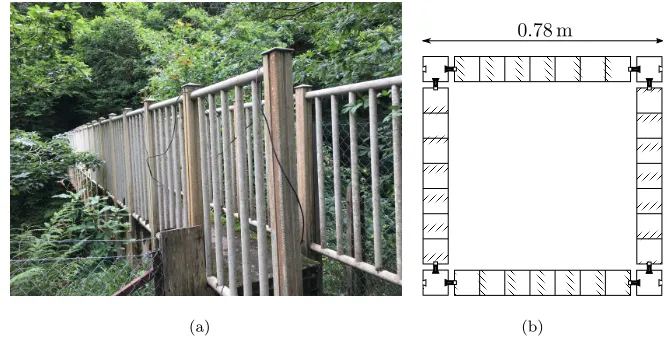
crosses a river valley (Fig. 1(a)). Pultruded fibre-reinforced polymer panels
interlock to form a square 0.78 m wide cross-section (Fig 1(b)). The bridge’s 70
total mass is approximately 1800 kg. Further details relating to the bridge can
be found elsewhere [15].
(a)
0.78 m
(b)
Figure 1: Lively footbridge (a) general view and (b) cross section of individual units that form the footbridge deck.
2.2. Modal testing
The current section summarises details about modal tests on the footbridge. 74
A detailed description of modal tests can be found in [15] and of FE
analy-sis in [16]. A modal test using an impact hammer was carried out to iden-76
tify vertical flexural and/or torsional vibration modes in the frequency range
up to 30 Hz. Additionally, the structure was excited by a pedestrian walking 78
at metronome controlled pacing rates from 1.40 Hz to 2.45 Hz in increments of
0.10 Hz or 0.05 Hz – depending of the pacing rate’s proximity to identified natu-80
ral frequencies. To check repeatability two walks were recorded for each pacing
rate. The vibration response was measured at two locations on the deck, and it 82
included recording of the free decay in the response after each crossing.
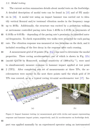
A measurement grid of 18 points (Fig.2(a)) was used to determine the modal 84
properties. Three roving accelerometers, one of which is shown in Fig. 2(b)
(model QA750 by Honeywell, nominal sensitivity of 1300 mVg−1), were used 86
to simultaneously measure response to hammer impact applied at test point
2 (TP2). After completing one set of measurements at three TPs, the ac-88
celerometers were moved to the next there points until the whole grid of 18
TPs was covered, as in a typical roving tri-axial accelerometer test [17].
Im-[m] 0.76 1 2 3 4 5 6 7 8 9 10 11 12
13 14 15
16 17 18
3.38 1.69 2.11 1.69 1.69 1.69 2.11 2.54 (a) (b)
Figure 2: Impact hammer testing (a) measurement grid with circles and square representing response and hammer impact points, respectively, and (b) accelerometer on footbridge deck. 90
pact was applied manually by an experienced operator using an instrumented
sledgehammer (model 5803A by Dytran, nominal sensitivity 0.23 mVN−1 and 92
tests, vertical responses were measured only at TP2 and TP5 at a sampling rate 94
of 256 Hz. All signals were acquired using a 24-bit, four channel Quattro (by
Data Physics) data logger and analyser. 96
The accelerance FRFs were calculated using six averages. Three flexural
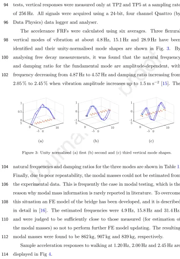
vertical modes of vibration at about 4.8 Hz, 15.1 Hz and 28.9 Hz have been 98
identified and their unity-normalised mode shapes are shown in Fig. 3. By
analysing free decay measurements, it was found that the natural frequency 100
and damping ratio for the fundamental mode are amplitude-dependent, with
frequency decreasing from 4.87 Hz to 4.57 Hz and damping ratio increasing from 102
2.05 % to 2.45 % when vibration amplitude increases up to 1.5 m s−2 [15]. The
(a) (b) (c)
Figure 3: Unity normalised (a) first (b) second and (c) third vertical mode shapes.
natural frequencies and damping ratios for the three modes are shown in Table1. 104
Finally, due to poor repeatability, the modal masses could not be estimated from
the experimental data. This is frequently the case in modal testing, which is the 106
reason why modal mass information is rarely reported in literature. To overcome
this situation an FE model of the bridge has been developed, and it is described 108
in detail in [16]. The estimated frequencies were 4.9 Hz, 15.8 Hz and 31.4 Hz,
and were judged to be sufficiently close to those measured (for estimation of 110
the modal masses) so not to perform further FE model updating. The resulting
modal masses were found to be 862 kg, 907 kg and 839 kg, respectively. 112
Sample acceleration responses to walking at 1.20 Hz, 2.00 Hz and 2.45 Hz are
displayed in Fig4. 114
f1 f2 f3(Hz) ζ1 ζ2 ζ3(%)
4.57-4.87 15.1 28.9 2.05-2.45 2.8 2.7
Table 1: Modal properties identified in impact hammer and free decay tests.
Figure 4: Acceleration responses of footbridge at TP2 and TP5 for three pacing rates at 1.20 Hz, 2.00 Hz and 2.45 Hz.
approach presented next. 116
3. Theoretical framework
The pedestrian-based approach is detailed in the following sections and is 118
illustrated in Fig.5. The core idea is to match power spectral densities (PSD)
of responses induced by a pedestrian on the bridge against theoretical PSDs. 120
The latter are based on forces obtained using a laboratory treadmill and a
probabilistic model of the structure. For the current work there is a eight years 122
gap between in-field and treadmill experiments. Although this is a significant
period of time, the test subject is well experienced in walking tests, has body 124
mass which hardly changed over time, and has been generating very much the
same peak responses when walking over structures similar to the one presented. 126
The to-be-identified modal properties – natural frequencies, damping ratios
and modal masses – are denoted asθ. The framework was implemented with 128
Figure 5: Diagram of spectral pedestrain-based approach.
3.1. Equation of motion – time domain 130
The general equation of motion of a structural system with Nd DOFs can
be written as follows 132
M¨y(t) +C ˙y(t) +Ky(t) =x(t) (1)
for a scenario of damped forced vibrations. M,C and K are Nd×Nd mass,
damping and stiffness matrices, ¨y,y,˙ y andx are Nd×1 time-dependent
vec-134
tors of acceleration, velocity, displacement and force induced by a pedestrian at
each DOF, respectively. Commonly this equation is transformed into its modal 136
equivalent by using the transformationy(t)Nd×1=ΦNd×nq(t)n×1 (forn
inde-pendent vibration modes), withΦ= [Φ1Φ2. . . Φn] defined as anNd×nmode
138
shape matrix. Pre-multiplying Eq. (1) by the transposed mode shape matrix
ΦTresults in 140
m¨q(t) + 2mζωnq˙(t) +mω2nq(t) =Φ
T
wherem,ζ,ωnare then-dimensional diagonal matrices that contain the modal
masses, damping ratios and circular natural frequencies, respectively. The vec-142
tor on the right-hand side represents time-dependent modal forces for given
modes, and q, q˙, ¨q are the modal response vectors of displacement, velocity 144
and acceleration, respectively. It should be noted that the mode shape matrix
on the RHS of Eq. (2) can be transformed from spatial to time domain using 146
t = l/v, where l is the longitudinal position of the pedestrian on the bridge
whilevis the pedestrian speed (assumed to be constant). 148
3.2. Frequency response function – frequency domain
In this section Eq. (1) is analysed in the frequency domain with the aid of 150
the Fourier transform (FT). Taking Eq. (2) as a basis, and applying the FT to
convert it from time into frequency domain, results in 152
m ¨Q(ω) + 2mζωnQ˙(ω) +mω2nQ(ω) =X(ω) (3)
where Q,¨ Q,˙ Q and X represent the FTs of the modal responses and modal
forces, respectively. In the present work the complex form of the FT is defined 154
as
X(ω) = 1 2π
Z ∞
−∞
x(t)e−iωtdt. (4)
By definition Q¨ = −ω2Q, Q˙ = iωQ and Q¨ = iωQ˙. The FT of the modal 156
acceleration response can be written as:
¨
Q(ω) =H(ω)X(ω). (5)
whereH is an n-dimensional diagonal FRF matrix, which is a function of the 158
structural modal properties. Accelerance FRF for a single degree of freedom
system is given by 160
H(ω) = −ω
2
m(−ω2+ω2
n+ 2ζiωnω)
. (6)
Now the FT of physical acceleration can be written as
¨
Assuming that the response has random fluctuations in it, anNd-dimensional
162
Hermitian PSD matrix at frequency ω can be obtained from the FT of the
response in Eq. (7) as follows 164
Sy¨(ω) = E[Y¨(ω)Y¨(ω)H] =ΦNd×nH(ω)n×nSX(ω)
n×nH(ω)H
n×nΦ
T
n×Nd, (8)
where SX is an n-dimensional Hermitian PSD matrix of modal forces. This
matrix contains in its diagonal and off-diagonal entries the auto and cross PSD 166
between modal forces, respectively. Eq. (8) is the central result of random
vibra-tion theory for a multiple DOF system, and it will be utilised as a data model 168
of the bridge-pedestrian system which allows to estimate modal properties.
4. Spectral model of the excitation
170
This section details how the PSD matrix of modal forces in Eq. (8) is
ob-tained. The following text adopts a discretised formulation whereby the PSD of 172
modal forces at frequencyk, sampled atN points at time interval ∆tis denoted
asSX,k (fk=k/(N∆t),k= 1, . . . , Nf), whereNf is the frequency bin number
174
correspondent to the Nyquist frequency of the discretised signal.
The modal force for each mode is calculated by weighting the time history 176
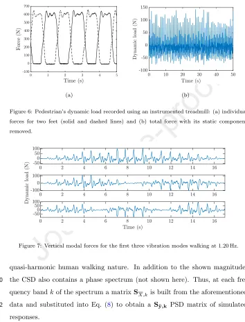
of force by the mode shape. Fig. 6(a) shows vertical component of walking
forces by each leg sampled at 200 Hz. The sum of the forces by two feet is then 178
calculated and the static weight is removed. The resulting dynamic force is
shown in Fig. 6(b). The force in this example is for walking at 1.20 Hz. The 180
modal forces for the three modes from Fig.3are shown in Fig.7.
The auto (ASD) and cross (CSD) spectral density terms of the modal forces 182
can now be determined. The CSD is a particularly relevant quantity, as it
highlights the correlations between different modal forces. 184
Assuming now that the modal forces are wide-sense stationary processes,
their PSDs can be estimated by multiplying their DFT with its complex con-186
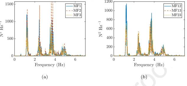
jugate. Fig.8shows an example of the calculated ASD and CSD of the modal
(a) (b)
Figure 6: Pedestrian’s dynamic load recorded using an instrumented treadmill: (a) individual forces for two feet (solid and dashed lines) and (b) total force with its static component removed.
Figure 7: Vertical modal forces for the first three vibration modes walking at 1.20 Hz.
quasi-harmonic human walking nature. In addition to the shown magnitude,
the CSD also contains a phase spectrum (not shown here). Thus, at each fre-190
quency bandkof the spectrum a matrix SX,kis built from the aforementioned data and substituted into Eq. (8) to obtain a S¨y,k PSD matrix of simulated 192
responses.
5. Probabilistic modal identification approach
194
This section details how the natural frequencies, damping ratios, and modal
(a) (b)
Figure 8: (a) Auto spectral density of modal forces and (b) cross spectral density of modal force pairs. The peaks represent the 1.20 Hz pacing rate and its higher harmonics.
5.1. Scaled discrete Fourier transform of observations
Let us assume that a given stochastic process, in this case the vibration 198
response of the bridge, has N time observations yej, j = 0, . . . , N −1 at Nd
observation channels. The process is dependent on modal propertiesθ, presented 200
in Section2.2, as well as on the PSD of the noise at each observation channel.
The scaled discrete Fourier transform (DFT) of the observations (frequency 202
fk=k/(N∆t)) is given by
Yk=
r
2∆t N
N−1
X
j=0
yeje−i2πjk/N (9)
where ∆tis the sampling time interval. The scaled DFTs on a selected frequency 204
band represent the core evidence used to identify the modal properties.
5.2. Likelihood function 206
The likelihood function is a joint probability density function (PDF) of a
collection of variables indexed by k {Yk} for given θ. Assuming long data,
208
{Yk}are (circularly symmetric) complex Gaussian and independent at different
frequencies. This gives 210
p({Yk}|θ) =
Y
k
where the product is taken over all frequencies in the selected band withNf
DFT points, assumed to be large compared to 1 (long data); and 212
p(Yk|θ) =
π−Nd
|Sk(θ)|
exp [−YHkSk(θ)−1Yk] (11)
whereSk(θ) is a theoretical PSD matrix of data (Hermitian) for a givenθ. The
complex Gaussian probability density function (PDF) in Eq. (10) is central to 214
the proposed modal analysis framework, as it holds for general stationary data
regardless of the frequency content of contributing activities. The latter affects 216
Sk(θ) but not the form of the PDF.
Next the derivation ofSk(θ) is detailed. Within a selected frequency band
218
k, the following model is assumed
Yk =Yˆk+εk (12)
where Yˆk and εk represent scaled DFTs of a theoretical structural dynamic
220
response and measurement noise, respectively. Similarly, the theoretical PSD of
the data is given by 222
Sk(θ) = E[YˆkYˆ
H
k|θ] + E[εkεHk|θ] (13)
assuming that the modal forces and the measurement noise are independent.
E[εkεHk|θ] = diag(S
1
e, Se2, . . . , SeNd), is a diagonal matrix, where each entry Sej
224
is the PSD of noise in the frequency band (assumed as constant) at the j-th
observation channel. Finally, the PSD of the structural response term can be 226
obtained from a modal contribution form, already presented in Eq. (8), and the
DFT of the structural dynamic responseYˆk is obtained from Eq. (7).
228
5.3. Log-likelihood function
Mainly for numerical reasons, it is common practice to work with the log-230
likelihood function (LFF) instead of the likelihood in Eq. (11), which can be
expressed as 232
`(θ) =−NdNflnπ−
X
k
ln|Sk(θ)| −
X
k
In order to identify the modal properties the LLF is sampled with the Metropolis–
Hastings (MH) algorithm [19]. The samples of θ indicate in which regions of 234
the parameter space the bridge-pedestrian model matches available data. In
addition to the likelihood maximum, the samples allow to compute other un-236
certainties, such as the variance of the estimate.
The current section is closed with a discussion of some numerical details. In 238
order to increase the numerical stability of the matrix inversion in Eq. (14), the
matrix is transformed with a Cholesky decomposition routine. Further details 240
of this operation are given inAppendix A.1. Relatively to the MH algorithm,
it is necessary to set a proposal probability distribution (proportional to the 242
target distribution), amongst other options which are summarised inAppendix
A.2. 244
6. Results and discussion
6.1. Numerical tests - constant modal properties 246
A large number of numerical tests have been run to assess the performance
of the pedestrian-based approach. Based on the results from Section2.2, fixed 248
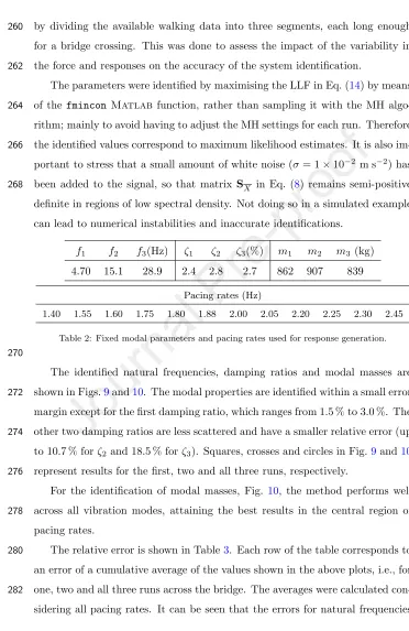
modal parameters were used to generate responses to walking at 12 pacing rates
(see Table2) usingMatlab. Each force time history measured on the treadmill 250
was weighted by the measured shape of each vibration mode (as in the RHS of
Eq. (2)) to determine modal forces for each mode. The modal forces were used 252
to calculate the modal responses in each individual vibration mode using the
Fox and Goodwin’s numerical procedure [20]. Then, the mode superposition 254
principle was employed to calculate the final acceleration response ¨yi(t) at a
locationion the deck, given by: 256
¨
yi(t) =
3
X
k=1
φi,kq¨k(t), (15)
whereφi,k is the amplitude of thekth mode shape (k= 1,2,3) at locationi(i=
1, . . . ,9) along the midline of the bridge (crosses in Fig. 2(a)) and ¨qk(t) is the
258
by dividing the available walking data into three segments, each long enough 260
for a bridge crossing. This was done to assess the impact of the variability in
the force and responses on the accuracy of the system identification. 262
The parameters were identified by maximising the LLF in Eq. (14) by means
of thefminconMatlab function, rather than sampling it with the MH algo-264
rithm; mainly to avoid having to adjust the MH settings for each run. Therefore
the identified values correspond to maximum likelihood estimates. It is also im-266
portant to stress that a small amount of white noise (σ= 1×10⁻² m s−2) has
been added to the signal, so that matrixSX in Eq. (8) remains semi-positive 268
definite in regions of low spectral density. Not doing so in a simulated example
can lead to numerical instabilities and inaccurate identifications.
f1 f2 f3(Hz) ζ1 ζ2 ζ3(%) m1 m2 m3 (kg)
4.70 15.1 28.9 2.4 2.8 2.7 862 907 839
Pacing rates (Hz)
1.40 1.55 1.60 1.75 1.80 1.88 2.00 2.05 2.20 2.25 2.30 2.45
Table 2: Fixed modal parameters and pacing rates used for response generation. 270
The identified natural frequencies, damping ratios and modal masses are
shown in Figs.9and10. The modal properties are identified within a small error 272
margin except for the first damping ratio, which ranges from 1.5 % to 3.0 %. The
other two damping ratios are less scattered and have a smaller relative error (up 274
to 10.7 % forζ2and 18.5 % forζ3). Squares, crosses and circles in Fig.9and10
represent results for the first, two and all three runs, respectively. 276
For the identification of modal masses, Fig. 10, the method performs well
across all vibration modes, attaining the best results in the central region of 278
pacing rates.
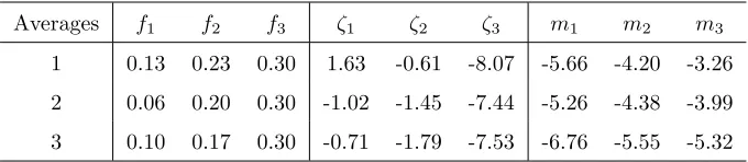
The relative error is shown in Table3. Each row of the table corresponds to 280
an error of a cumulative average of the values shown in the above plots, i.e., for
one, two and all three runs across the bridge. The averages were calculated con-282
(a) (b) (c)
(d) (e) (f)
Figure 9: Identified (a-c) natural frequencies and (d-f) damping ratios at several pacing rates for first (squares), second (crosses) and third runs (circles), and their true value (horizontal dashed line).
(a) (b) (c)
Figure 10: Identified (a–c) modal masses at several pacing rates for first (squares), second (crosses) and third runs (circles), and their true value (horizontal dashed line).
are negligible and the largest absolute value for the error is about 8 % for ζ3. 284
There is no significant error improvement beyond a single run across the bridge.
This error is a consequence of treating the measured signals as wide sense sta-286
tionary in Eq. (8). The error can be said to be sufficiently small for practical
Averages f1 f2 f3 ζ1 ζ2 ζ3 m1 m2 m3
1 0.13 0.23 0.30 1.63 -0.61 -8.07 -5.66 -4.20 -3.26
2 0.06 0.20 0.30 -1.02 -1.45 -7.44 -5.26 -4.38 -3.99
3 0.10 0.17 0.30 -0.71 -1.79 -7.53 -6.76 -5.55 -5.32
Table 3: Relative error (%) of identifications for an increasing number of runs averages.
Parameter α0 α1 α2 α3 α4 α5
f1 Hz 4.872 −0.4958 0.3387 −0.1227 0.02112 −0.001364
ζ1 % 2.073 1.167 −1.368 0.6789 −0.1526 0.012 35
Table 4: Polynomial regression coefficients of amplitude-dependent modal properties.
6.2. Numerical tests - amplitude-dependent modal properties
This section highlights a more challenging simulated example of modal iden-290
tification with amplitude-dependent modal properties. In an attempt to emulate
the real behaviour of the footbridge, the first natural frequency and damping 292
ratio were modelled as amplitude-dependent. Specifically, they were modelled
as 5th order polynomial functions of the peak acceleration (see Table4) as ob-294
tained fitting free-decay data. The equation of motion was solved by using Fox
and Goodwin’s numerical procedure [20]. Since the damping ratio and natural 296
frequency of the first mode are functions of vibration amplitude (Table4), their
values for simulating the response in the next vibration cycle are taken using 298
maximum absolute values from the previous cycle. When simulating response
in the first cycle, the values of 4.872 Hz and 2.073 % were used (free coefficients 300
in Table4). All the other modal parameters were kept constant, as defined in
the previous section. 302
The identified natural frequencies are shown in Fig. 11. The shaded area
in Fig. 11(a)shows an actual range of natural frequencies that corresponds to 304
the vibration amplitude range. The identified natural frequency lies within the
area, i.e., the method approximates the amplitude-dependent natural frequency 306
section, the other natural frequencies are identified within a small error margin 308
(up to 1.99 % forf2 and 1.38 % forf3).
(a) (b) (c)
Figure 11: Identified (a–c) natural frequencies at several pacing rates for first (squares), second (crosses) and third runs (circles) and their true values (shaded area and horizontal dashed lines).
Fig. 12 shows the identified damping ratios and modal masses. Similarly 310
to the previous section, modal masses are identified in a consistent manner
across all three vibration modes, whereas the first damping ratio has a larger 312
variability across pacing rates than the other two ratios. Compared with the
results in the previous section the estimate of damping ratios identification 314
have worsened, which suggests that identification of these modal properties is
susceptible to nonlinear effects. For the modal masses, Figs. 12(d)12(e)12(f)
316
indicate a reliable estimation within a central band, from 1.75 Hz to 2.20 Hz
of the pacing rates, while the results are more erroneous for pacing rates at 318
1.55 Hz and 2.30 Hz, whose third and second harmonic, respectively, are close to
the natural frequency of the first mode. In the authors’ opinion, the reason is 320
that close peaks are present in the spectrum in these tests and the identification
becomes sensitive to frequency resolution of the signal, which is particularly 322
coarse in case of faster walking (when the time domain signal is shorter).
As in the previous section, the relative error of the identifications is shown 324
in Table 5. For the amplitude-dependent modal properties, the “true” value
was considered as the mid-value of the lines that outline the shaded areas in 326
Figs. 11(a) and 12(a). For the current example the damping ratios have the
(a) (b) (c)
(d) (e) (f)
Figure 12: Identified (a-c) damping ratios and (d-f) modal masses at several pacing rates for first (squares), second (crosses) and third runs (circles), and their true value (shaded areas and horizontal dashed lines).
tween the average error with one or more runs across the bridge.
Averages f1 f2 f3 ζ1 ζ2 ζ3 m1 m2 m3
1 -0.82 0.06 0.19 18.16 -3.26 -11.24 -3.03 -3.67 -4.44
2 -0.96 0.06 0.18 21.04 -3.87 -10.06 -3.12 -4.88 -5.91
3 -1.00 0.05 0.17 20.55 -3.89 -9.41 -4.20 -5.75 -6.90
Table 5: Relative error (%) of identifications for an increasing number of runs averages.
6.3. Measurements on the footbridge 330
In this section acceleration data measured at TP2 and TP5 on the actual
footbridge (Fig. 4) are used for validation of the pedestrian-based approach. 332
Results will be compared against measured modal properties reported in
Sec-tion2.2. 334
The MH algorithm was fine-tuned to obtain the distribution of the modal
samples. Since the data in Sections 2.2 and 4 were sampled at 256 Hz and
200 Hz, respectively, the former has been resampled down to 200 Hz, so that the 338
theoretical and experimental PSD responses have the same frequency resolution.
The results related to walking at 1.40 Hz, 1.55 Hz, 1.60 Hz, 1.75 Hz, 1.80 Hz, 340
1.88 Hz, 2.00 Hz, 2.05 Hz, 2.25 Hz, 2.30 Hz and 2.45 Hz are presented.
One of the differences relative to the previous numerical examples is that 342
the measured vibration response is caused by a force generated by a person
walking over the bridge that inevitably differs from the treadmill force used in 344
the analysis [21,22].
The estimated natural frequencies and damping ratios are shown in Fig.13. 346
The error bars represent a 99.7 % confidence interval of the estimate computed
from the MH samples, and the squares and crosses represent the identified mean 348
value for the first and second run, respectively. The identifications of the second
(a) (b) (c)
(d) (e) (f)
Figure 13: Identified (a-c) natural frequencies and (d-f) damping ratios, mean values (circles) and 99.7 % confidence intervals (error bars) for different pacing rates. The reference values are the shaded area and horizontal dashed lines.
and third damping ratio are biased because of their sensitivity to nonlinearities 350
is slightly offset from the pedestrian’s step rate on the bridge, there is an off-352
set between the harmonics of these two types of excitation, which would be
increasingly larger the higher the harmonic is. Thus, higher frequencies are 354
more affected by intra-subject variability than lower frequencies, which agrees
with the presented results for the second/third and the first damping ratio, 356
respectively.
To further minimise errors, the time lag between treadmill and in-field 358
recordings should also be as small as possible, especially if the test subject
is inexperienced with walking tests. 360
Lastly, the modal masses identification is shown in Fig.14. The error has
increased in comparison with the numerical examples, but it is still within 30 % 362
mark achieved when using other more elaborate test setups. The increase in
this error is partially due to uncertainty of the actual modal masses associated 364
with estimating them using the FE model.
(a) (b) (c)
Figure 14: Identified (a–c) modal masses mean values (circles) and 99.7 % confidence intervals (error bars) at several pacing rates. Their reference values are the horizontal dashed lines.
The relative errors are presented in Table6. The maximum absolute value of 366
the error is up to 3 %, 69 % and 22 % for natural frequencies, damping ratios and
modal masses, respectively. The main difference comparatively to the numerical 368
examples is the more pronounced bias of the identified second and third damping
ratios. 370
The errors for natural frequencies and modal masses are sufficiently small
to be competitive against other types of tests (shaker, impact hammer and 372
Averages f1 f2 f3 ζ1 ζ2 ζ3 m1 m2 m3
1 2.94 -1.62 -0.61 -1.79 -58.61 -65.61 -29.25 3.94 -26.06
2 2.23 -1.47 -0.52 -6.28 -58.99 -68.97 -22.03 6.15 -20.97
Table 6: Relative error (%) of average of identifications for field measurements.
in data collection using the proposed method and promising nature of the results 374
suggest that the method has potential to be used in system identification and
it is worth investigating and improving further in future research. 376
7. Conclusions
An approach, with potential to identify modal properties using a pedestrian 378
excitation, has been developed and applied to a lightweight FRP footbridge.
The approach was validated against both numerical and field data. 380
The methodology was found to provide reliable modal properties estimates,
with the exception of damping ratios when considering a structure with amplitude-382
dependent behaviour. Generally, the best results are obtained with pacing rates
that are not close to the structure’s resonant frequency. Additionally, pre-384
liminary numerical tests (not presented here) indicate that the approach can
be applied to heavier and less responsive bridges with similar error margins. 386
Therefore, future work is required to explore the extents of the methodology.
The proposed model can be further developed by replacing the treadmill-388
based pedestrian walking forces by a probabilistic model of an overground
walker; or by enhancing the proposed statistical model to account for model 390
bias and human-structure interaction effects; and reimplementing the approach
on the basis of a structure with amplitude-dependent behaviour to improve the 392
identification of damping ratios.
Nevertheless, the reported errors for natural frequencies and modal masses 394
are sufficiently small comparatively to the typically used tests. Thus, the
pedestrian-based approach’s reliability, cost-effectiveness and simplicity further 396
Acknowledgements
398
The authors would like to thank the anonymous reviewers/editor and Julia
Dinan for feedback on the manuscript. The research in this paper was partially 400
supported by the UK Engineering and Physical Sciences Research Council (grant
number EP/M021505/1 Characterising dynamic performance of fibre reinforced 402
polymer structures for resilience and sustainability).
Appendix A. Computational aspects
404
Appendix A.1. Cholesky decomposition
This section details some of the computational aspects of the proposed frame-406
work. Although matrixSk(θ) in Eq. (11) is not expected to be very large – its
dimension corresponds to the number of DOF – it can become ill-conditioned. 408
Furthermore, determining its inverse and determinant can be computationally
costly. The current approach exploits the fact that it is an Hermitian semi-410
positive definite matrix, and therefore, can be factorised with the Cholesky
decomposition as 412
Sk(θ) =C(θ)C(θ)H, (A.1)
withC(θ) as a lower triangular matrix. This transformation allows an
orthog-onal transformation from the generalised to ordinary least squares solution of 414
the overdetermined system to be performed:
Ck(θ)Yek =Yk. (A.2)
Having presented the factorisation, the original datasetY and the PSD matrix 416
of the theoretical model can now be very simply replaced by their transformed
equivalents to simplify the likelihood functions shown in the original formula-418
tion. Thus, Eq. (11) becomes
p(Yk|θ) =
π−Nd
|Ck(θ)|2
exp [−Ye
H
kYek] (A.3)
and Eq. (14) becomes 420
`(θ) =−NdNflnπ−2
X
k
ln|Ck(θ)| −
X
k
e
Appendix A.2. Details of the Metropolis–Hastings algorithm
The Metropolis–Hastings algorithm belongs to the class of Markov Chain 422
Monte Carlo (MCMC) algorithms, that approximate a target multi-dimensional
probability distribution with a large number of samples. The algorithm has to be 424
fine-tuned so that the obtained samples reflect the target distribution faithfully,
i.e. regions of low probability density are visited less frequently by the sampling 426
routine than regions of high density. In the context of the current work, each
dimension of the sampled target distribution corresponds to one of the modal 428
properties and noise PSD.
An important aspect of the whole procedure is the correlation between iden-430
tified modal parameters, which has to be as low as possible. An indicator of the
correlation between modal properties marginal PDFs is the correlation matrix, 432
defined as
R(θ) = (diag(Σ))−12Σ(diag(Σ))− 1
2, (A.5)
whereΣis the modal parameters covariance matrix, and diag(Σ) is a diagonal 434
matrix of the elements of Σ. The entries of the correlation matrix represent
the Pearson coefficients, i.e. the linear dependency between the parameters, 436
with a−1,0,1 representing a perfectly negative, lack of, or perfectly positive
correlation between parameters, respectively. 438
Furthermore, three other options have to be set:
1. a proposal distribution that guides where the Markov chain will move at 440
each iterative step;
2. a random generator routine for each of the sampled parameters; 442
3. the number of burn-in samples, to skip low probability density regions
during the initial steps of the chain; 444
In the current work, a uniform distributiong has been adopted as the proposal
distribution, within an interval [−δ;δ] as follows 446
g(θ0|θ) =
1
2δ for −δ≤θ−θ
0≤δ
0 forθ−θ0<−δorθ−θ0 > δ
where θ and θ0 correspond to a current and newly generated sample of the
modal properties, respectively. The random sample generator was also assumed 448
as a uniform sampling grid, centred atθand within a±δinterval. The burn-in
period was set as 2000 for a total amount of 10 000 samples of a symmetric 450
target distribution.
The factor with more influence in the correlation of the samples and conver-452
gence speed of the MH algorithm is the proposal distribution’s jumping width
vector, δ. The jumping width must be large enough so that the modal pa-454
rameters are not excessively correlated. In a scenario when there is a trade-off
between a reasonable acceptance rate and uncorrelated modal parameters, it is 456
necessary to increase the total amount of samples and involved computational
effort. 458
References
[1] J. Brownjohn, P. Reynolds, S.-K. Au, D. Hester, M. Bocian, Experimental 460
modal analysis of civil structures: State of the art, in: SHMII – 7th
International Conference on Structural Health Monitoring of Intelligent 462
Infrastructure, 2015.
[2] E. Caetano, ´A. Cunha, Modal Testing of the Vasco daGama Bridge, Por-464
tugal, in: C. Boller, F.-K. Chang, Y. Fujino (Eds.), Encyclopedia of
Struc-tural Health Monitoring, John Wiley & Sons, Ltd, Chichester, UK, 2008. 466
doi:10.1002/9780470061626.shm168.
[3] F. Magalh˜aes, E. Caetano, ´A. Cunha, O. Flamand, G. Grillaud, Ambient 468
and free vibration tests of the Millau Viaduct: Evaluation of alternative
processing strategies, Engineering Structures 45 (2012) 372–84. 470
[4] S.-K. Au, Uncertainty law in ambient modal identification—Part I: Theory,
Mechanical Systems and Signal Processing 48 (2014) 15 – 33. 472
Im-plication and field verification, Mechanical Systems and Signal Processing 474
48 (2014) 34 – 48.
[6] C. W. Kim, M. Kawatani, J. Hao, Modal parameter identification of short 476
span bridges under a moving vehicle by means of multivariate AR model,
Structure and Infrastructure Engineering 8 (2012) 459–72. 478
[7] P. Reynolds, A. Pavic, Impulse Hammer Versus Shaker Excitation for the
Modal Testing of Building Floors, Experimental Techniques 24 (2000) 39– 480
44.
[8] R. R. Craig, A. Kurdila, R. R. Craig, Fundamentals of Structural Dynam-482
ics, 2nd ed ed., John Wiley, Hoboken, N.J, 2006. OCLC: ocm61247316.
[9] S.-K. Au, Operational Modal Analysis, Springer Berlin Heidelberg, New 484
York, NY, 2017.
[10] J. Brownjohn, A. Pavic, Experimental methods for estimating modal mass 486
in footbridges using human-induced dynamic excitation, Engineering
Struc-tures 29 (2007) 2833–43. 488
[11] J. M. W. Brownjohn, M. Bocian, D. Hester, A. Quattrone, W. Hudson,
D. Moore, S. Goh, M. S. Lim, Footbridge system identification using wire-490
less inertial measurement units for force and response measurements,
Jour-nal of Sound and Vibration 384 (2016) 339–55. 492
[12] G. Piccardo, F. Tubino, Equivalent spectral model and maximum dynamic
response for the serviceability analysis of footbridges, Engineering Struc-494
tures 40 (2012) 445–56.
[13] K. Lievens, G. Lombaert, K. Van Nimmen, G. De Roeck, P. Van den 496
Broeck, Robust vibration serviceability assessment of footbridges subjected
to pedestrian excitation: Strategy and applications, Engineering Structures 498
[14] E. Shahabpoor, A. Pavic, V. Racic, Identification of walking human model 500
using agent-based modelling, Mechanical Systems and Signal Processing
103 (2018) 352–67. 502
[15] X. Wei, J. Russell, S. ˇZivanovi´c, J. Toby Mottram, Measured dynamic
properties for FRP footbridges and their critical comparison against struc-504
tures made of conventional construction materials, Composite Structures
223 (2019) 110956. 506
[16] X. Wei, H.-P. Wan, J. Russell, S. ˇZivanovi´c, X. He, Influence of
mechan-ical uncertainties on dynamic responses of a full-scale all-FRP footbridge, 508
Composite Structures 223 (2019) 110964.
[17] B. J. Schwarz, M. H. Richardson, Experimental modal analysis, in: In 510
Proceedings of CSI Reliability Week, 1999.
[18] A. Jesus, Data for: A spectral pedestrian-based approach for modal iden-512
tification, 2019. doi:10.17632/cj7353cc9j.1.
[19] I. Yildirim, Bayesian Inference: Metropolis-Hastings Sampling, Dept. of 514
Brain and Cognitive Sciences, Univ. of Rochester, Rochester, NY (2012).
[20] L. Fox, E. T. Goodwin, Some new methods for the numerical integra-516
tion of ordinary differential equations, Mathematical Proceedings of the
Cambridge Philosophical Society 45 (1949) 373–88. 518
[21] J. Chen, J. Wang, J. M. W. Brownjohn, Power Spectral-Density Model for
Pedestrian Walking Load, Journal of Structural Engineering 145 (2019) 520
04018239.
[22] M. Garc´ıa-Di´eguez, J. Zapico-Valle, Statistical modelling of spatiotem-522
poral variability of overground walking, Mechanical Systems and Signal