City, University of London Institutional Repository
Citation:
Tomas-Rodriguez, M. and Banks, S. P. (2013). An iterative approach to eigenvalue assignment for nonlinear systems. International Journal of Control, 86(5), pp. 883-892. doi: 10.1080/00207179.2013.765037This is the unspecified version of the paper.
This version of the publication may differ from the final published
version.
Permanent repository link:
http://openaccess.city.ac.uk/2430/Link to published version:
http://dx.doi.org/10.1080/00207179.2013.765037Copyright and reuse: City Research Online aims to make research
outputs of City, University of London available to a wider audience.
Copyright and Moral Rights remain with the author(s) and/or copyright
holders. URLs from City Research Online may be freely distributed and
linked to.
City Research Online: http://openaccess.city.ac.uk/ [email protected]
An Iterative Approach to Eigenvalue Assignment
for Nonlinear Systems.
M.Tomas-Rodriguez
a∗and S.P.Banks
ba
The City University, School of Engineering and Mathematical Sciences, London, UK.
b
Automatic Control and Systems Engineering Department, The Sheffield University,
UK.
Abstract
In this paper, the authors present a method for controlling a nonlinear system by using the ideas of eigenvalues assignment. A time-varying approach to nonlinear exponential stability via eigenvalue placement is studied based on an iteration technique that approaches a nonlinear system by a sequence of linear time-varying equations. The convergent behaviour of this method is shown and applied to a practical nonlinear example in order to illustrate these ideas.
Index Terms
Nonlinear systems, Eigenstructure Assignment, Pole placement, Iteration.
I. INTRODUCTION
The aim of this paper is to design a feedback controller so that the original nonlinear system is stabilized according to some requirements. The pole placement idea for linear time invariant systems is extended to a general pole placement technique applicable to linear time-varying systems and with the aid of an iteration technique presented in [Tomas-Rodriguez et al.(2003)], ultimately to nonlinear systems in a general form. Several authors approached the pole placement idea for general nonlinear systems in the past; Most of these techniques have in common the idea of linearizing the nonlinear system about a countable set of equilibrium points and finding a single controller that will stabilize each member of the finite countable set (see [Chow(1990)] for example). On the other hand, within the area of nonlinear systems, and having its origins in the geometric control theory, exact feedback linerization with pole placement is achieved by following a two-step design method as in [Isidori(1989)] and [Sontag(1998)]. There have been as well attempts to obtain both feedback linearization and pole placement objectives in just one step as in [Kazantzis et al.(2000)].
Pole placement for linear time invariant systems has been the object of diverse studies: Some of them were based on Ackerman′
s formula [Ackermanet al.(1972)], others approached the problem by using a periodic output feedback ([Greschak et al.(1990)], [Aeyels et al.(1991)]) for second order systems or even arbitrary order as in [Aeyels et al.(1992)].
The original pole placement method for linear time invariant SISO systems was first extended to linear time-varying systems by [Silverman(1966)] using a canonical representation of the original system. Since then, it had been several contributions by different authors to develop pole placement techniques for linear time-varying systems (i.e. [Silverman(1966)], [Tuel(1967)], [Luenberger(1967)], [Kailath(1980)], [Varga(1981)], [Miminis(1982)], [Petkov et al.(1985)], [Kautsky et al.(1985)], [Choi(1995)], [Choi(1996)], [Choi(1998)] or [Bhattacharyya et al.(1982)]). More recently, Valasek et.al. initiated
a series of publications related to the eigenvalue placement problem based on the extension of Ackerman′
s formula to linear time-varying SISO and later to linear time invariant and linear time-varying M IM O systems in which the eigenvalue placement was based on the equivalence of the closed-loop original system via a Lyapunov transformation to a linear time invariant system with poles at prescribed locations ([Valasek et al.(1995)], [Valasek et al.(1995b)], [Valasek et al.(1999)]). It should be pointed out that an important limitation of the pole placement algorithm is the lack of guaranteed tracking performance. This topic is treated in more general output feedback approaches. A typical remedy for this involves the incorporation of the Internal Model Principle into the control law design ([Francis et al.(1976)] and [Bengtsson(1977)]) or the inclusion of integrators into the loop. This issue will not be addressed in this paper, since pole placement design is the main interest here.
The contents of this article are based on the classical pole placement method for linear time invariant
systems and the iteration technique presented in [Tomas-Rodriguez et al.(2003)], [Tomas-Rodriguez et al.(2010)]. The objective is to develop a pole placement method for nonlinear systems of the form:
˙
x=f(x) =A(x)x(t) +B(x)u(t), x(0) =x0.
Replacing the nonlinear system above by a sequence of linear time-varying systems, a sequence of feedback laws of the form u(i)(t) =K(i)(t)x(i)(t)can be generated: for each of them, the closed-loop
poles for the ith linear time-varying system at each time of the time interval are allocated to some desired location σ = (λ1d,· · ·λnd) where each λi can be time-varying or constant. This iteration technique is presented in Section II.
It is well-known that linear time-varying systems can be unstable despite having left half-plane poles; that is, for linear time-varying systems, poles do not have the same stability meaning as in the time invariant case, so the allocation of the pole in the left hand side plane does not guarantee the stability of the closed-loop system. In order to overcome this problem an approach to stability using Duhamel’s principle is presented in Section III where conditions based on differentiability of the eigenvector′
s matrix are derived.
From the convergence properties of the sequence of linear time-varying solutions, [Tomas-Rodriguez et al.(2003)], by choosing theK(i)(t)feedback gain corresponding to theithiteration and applying the limiting value
to the closed-loop nonlinear system, the pole placement and stability objectives are achieved for a wide variety of nonlinear cases. This generalization to nonlinear systems is given in Section IV, followed by a numerical example in Section V. Section VI contains the conclusions and further research guidelines.
II. ITERATION TECHNIQUE FOR NONLINEAR SYSTEMS
This section recalls a recently introduced technique for nonlinear dynamical systems in which the original nonlinear equation is replaced by a sequence of linear time-varying equations converging in the space of continuous functions to the solution of the nonlinear system under a mild Lipschitz condition [Tomas-Rodriguez et al.(2003)]. This method has also been used in optimal control theory [Tomas-Rodriguez et al.(2005)], in the design of nonlinear observers [Navarro-Hernandez et al.(2003)] or control of a super-tanker [Tayfun Cimen et al.(2004)] to cite a few. Any nonlinear system of the form
˙
x=f(x) = A(x)x, x(0) = x0 ∈Rn. (1)
whereA(x) is locally Lipschitz can be approximated by a sequence of linear time-varying equations:
˙
x(1) =A[x(0)]x(1), x(1)(0) =x(0)
.. .
˙
x(i) =A[x(i−1)
]x(i), x(i)(0) =x(0)
(2)
of the nonlinear system given in (1). The convergence of these sequence is stated in the following theorem:
Suppose that the nonlinear equation (1) has a unique solution on the interval [0, τ] denoted by x(t)
and assume that A : Rn → Rn is locally Lipschitz. Then the sequence of functions defined in (2) converges uniformly on [0, τ] to the solution x(t).
The convergence of Theorem II is proved in [Tomas-Rodriguez et al.(2003)] where global conver-gence is extended to time intervals t ∈ [0,∞]. The application of this technique gives an accurate representation of the nonlinear solution after a few iterations. Nonlinear systems satisfying the local Lipschitz requirement can be now approached by common linear techniques. This is a very mild assumption, and is already assumed for the uniqueness of solution in Theorem II.
III. EIGENVALUE ASSIGNMENT FOR LINEAR TIME-VARYING SYSTEMS
A. General approach to pole placement
In this section the pole-placement method for linear time invariant cases will be extended to linear time-varying systems of the form:
˙
x(t) =A(t)x(t) +B(t)u(t), x(0) =x0 (3)
where x(t) ∈ Rn is the vector of the measurable states, u(t) ∈ Rm is the control signal and A(t),
B(t) are time-varying matrices of appropriate dimensions. Given a set of desired stable eigenvalues, σ = λ1d· · ·λnd
and a time interval [0, t], the aim is to place the closed-loop eigenvalues of (3) at those desired points ∀t∈(0, t)by using a convenient state feedback control u(t) = −K(t)x(t) where the feedback gain K(t) is a time dependent function.
Given that the pair hA(t), B(t)i is controllable for all t∈[0, t], the eigenvalue placement theorem is applied to (3):
detλ·I−[A(t)−B(t)K(t)]= (λ−λ1d)· · ·(λ−λnd) (4)
and by solving (4), a time-varying feedback gainK(t)can be determined so that the closed-loop form of the system (3) will now be of the form
˙
x(t) = [A(t)−B(t)K(t)]x(t) = ˜A(t)x(t) (5)
with stable eigenvalues on the left-half plane at λ1· · ·λn
= λ1d· · ·λnd
. In order to guarantee stability of the system (3), further issues should be taken into account as for linear time-varying systems, the existence of negative closed-loop poles is not a sufficient condition for stability.
In the following sections, conditions for exponential stability of linear time-varying systems with negative eigenvalues will be derived and these results will be extended for the nonlinear case.
B. Sufficient stability conditions for linear time-varying systems
Having in mind that the matrixAe(t)already has negative eigenvalues by (4), some other conditions for stability of the closed-loop system (5) should be satisfied, these conditions can be summarized in the following theorem: Given the open loop linear time-varying system x˙ =A(t)x(t) +B(t)u(t),
x0 =x(0), whose closed-loop matrixAe(t) =A(t)−B(t)K(t)has designed left hand-plane eigenvalues
σ= (λ1d, . . . , λnd) via the feedback signal u(t) =−K(t)x(t) and assuming the following conditions
to be satisfied:
I/ λ1d is the eigenvalue of Ae(t) with the greatest real part, II/ The matrix of eigenvectors P(t) is differentiable,
III/ ||P−1
then for β < Re(λ1d) the closed-loop system
˙
x= [A(t)−B(t)K(t)]x(t) = Ae(t)x(t)
is exponentially stable.
Proof: The system (5) can be solved over any time interval [0, t], by dividing the interval into N
subintervals of length h, such that h=t/N →0 when N → ∞, using Duhamel′
s principle,
x(t) = limh→0
eA˜[N h]h·eA˜[(N−1)h]h
. . . eA˜[h]h·I ·x
0
(6)
Applying the similarity transform eAe(t) =P(t)eΛ(t)P−1
(t) to (6) yields:
x(t) = PNeΛ[N h]hP
−1
N
·PN−1eΛ[(
N−1)h]h
P−1
N−1
· · ·P1eΛ[h]hP −1 1
·I·x0 (7)
where Λ(t)∈Cnxn is a diagonal matrix of desired eigenvalues and P(t)∈ Cnxn is the time-varying matrix of the corresponding eigenvectors.
PN is P(t) at time t =N h.
Λ(t) is considered to be time-varying to generalize the results of Theorem III-B. In this particular article it is considered to be constant as the desired eigenvalues were taken to be constant.
The second assumption was thatP(t) was differentiable, therefore its Taylor expansion will be of the form:
P(t+h) = P(t) +hdP(t)
dt +
h2
2!
d2P(t)
dt +· · · (8)
Neglecting high order terms and noting that dPdt(t) = ˙P(t):
P(t+h) =P(t) +hP˙(t) (9)
By inverting both sides of equation (9), post-multiplying by P(t) and, using the approximation
(1 +a)−1
≈1−a+· · ·, we obtain:
P(t+h)−1
P(t)≈hI−P(t)−1
hP˙(t)i (10)
and,
P(t+h)−1
·P(t)≈I+ǫ(h) (11)
where ǫ=o(h), so that ǫ→0 as h→0.
Thus, (7) can be written as:
x(t) = PN ·eΛ[N h]h·(I+ǫ)·eΛ[(N
−1)h]h·(I+ǫ)· · ·eΛ[h]hP
1·I ·x0 (12)
Taking norms of the above expression, a bound on the norm of x(t) can be estimated by,
||x(t)|| ≤ ||PN|| · ||(1 +ǫ)||N · ||P1|| · ||e(Λt)|| · ||x0|| (13)
and taking into account that
||eΛt|| ≤eRe(−λmax)t
where λmax is the eigenvalue of the matrix Λ with largest real part, then for λmax =λ1d
||x(t)|| ≤ ||PN|| · ||(I+ǫ)||N · ||P1|| ·e −λ1dt
· ||x0||. (14)
Now, it was shown in (11) that ǫ(h) = −hP−1
(t) ˙P(t), so
||I +ǫ||=||I−hP−1 ˙
P(t)|| ≤1 +h||P−1
By Assumption III in Theorem III-B, ||P−1
(t) ˙P(t)|| is bounded by β, and ||I+ǫ(h)|| ≤1 +hβ.
Therefore,
||x(t)|| ≤ ||PN|| ·(1 +hβ)N · ||P1|| ·e −λ1dt
· ||x0||
and
(1 +hβ)N = 1 + βt
N
!N
→eβt
so
||x(t)|| ≤ ||PN|| ·e(β
−λ1d)t
· ||P1|| · ||x0||.
Analyzing the expression above for exponential stability, PN, P1, and x0 are constant values, so
et(β−λ1d)
→0 is required:
e(β−λ1d)t
→0, (β−λ1d)<0→β <|λ1d|. (15)
That is, for exponential stability, the closed-loop eigenvalues λd should be chosen so that the greatest of them λ1d satisfies (15) which represents a compromise between the upper bound of the rate of change of P(t) and λ1d.
C. A Necessary condition for the differentiability of P(t)
In the previous section it was shown how the exponential stability properties of the closed-loop system relied upon the satisfaction of conditions I-III in Theorem III-B. These conditions were sufficient conditions for stability. In this section a necessary condition for stability will be derived. This condition is given in terms of a differential equation which places restrictions on Λ(t), K(t)and
P(t). The necessary condition for stability is stated as follows: The differentiability of the matrix of eigenvectors P(t) (and A(t), B(t), K(t) and Λ(t)) imply that the following equation is satisfied:
h ˙
A(t)−B˙(t)K(t)−B(t) ˙K(t)i=P(t)h˙Λ(t)−Λ(t)P−1
(t) ˙P(t) +P−1
(t) ˙P(t)Λ(t)iP−1
(t), (16)
where Λ(t) is the diagonal matrix of eigenvalues of A(t) and K(t) is the feedback gain designed for stable closed loop poles. Proof: Consider two nearby time points t and t+h, and evaluate the similarity transforms at those points keeping in mind that the matrix Λ(t) is a diagonal matrix containing the eigenvalues of the matrix hA(t)−B(t)K(t)i= ˜A(t):
P−1
(t) [A(t)−B(t)K(t)]P(t) = Λ(t) (17)
P−1
(t+h) [A(t+h)−B(t+h)K(t+h)]P(t+h) = Λ(t+h) (18)
as in (8) and the assumed differentiability of A(t), B(t) and K(t). Then,
A(t+h) =A(t) +hA˙(t) +· · ·
B(t+h) = B(t) +hB˙(t) +· · ·
K(t+h) = K(t) +hK˙(t) +· · ·
and by the differentiability of P(t) and (10);
P−1
(t+h) =P−1
(t)−hP−1
(t) ˙P(t)P−1
(t)
it follows that (18) can be written as
Λ(t+h) = hP−1
(t)−hP−1
(t) ˙P(t)P−1
(t)i·hA(t) +hA˙(t)−B(t) +hB˙(t)·K(t) +hK˙(t)i·
Expanding and rejecting high order terms yields:
Λ(t)+h˙Λ(t) = hP−1
(t)−hP−1
(t) ˙P(t)P−1
(t)i·hA(t)+hA˙(t)−B(t)K(t)−hB˙(t)K(t)−hBK˙(t)i·hP(t)+hP˙(t)i
this is,
Λ(t) +h˙Λ(t) =P−1
(t)hA(t)−B(t)K(t)iP(t) +P−1
(t)hhA(t)−B(t)K(t)iP˙(t)
+P−1
(t)hhA˙(t)−B˙(t)K(t)−B(t) ˙K(t)iP(t)−hP−1
(t) ˙P(t)P−1
(t)hA(t)−B(t)K(t)iP(t).
(19) Taking into account thatP−1
(t)hA(t)−B(t)K(t)iP(t) = Λ(t) andP−1
(t)hhA(t)−B(t)K(t)iP˙(t) =
hΛ(t)P−1
(t) ˙P(t), now equation (19) can be written as:
Λ(t)+h˙Λ(t) = Λ(t)+hΛ(t)P−1
(t) ˙P(t)−hP−1
(t) ˙P(t)Λ(t)+hP−1
(t)hA˙(t)−B˙(t)K(t)−B(t) ˙K(t)iP(t).
Dividing by h on both sides a differential equation in Λ(t) is obtained:
˙Λ(t) = P−1
(t)hA˙(t)−B˙(t)K(t)−B(t) ˙K(t)iP(t) + Λ(t)P−1
(t) ˙P(t)−P−1
(t) ˙P(t)Λ(t) (20)
or
P−1
(t)hA˙(t)−B˙(t)K(t)−B(t) ˙K(t)iP(t) = ˙Λ(t)−Λ(t)P−1
(t) ˙P(t) +P−1
(t) ˙P(t)Λ(t). (21)
Multiplying on the left by P−1
(t) and on the right by P(t), then:
h ˙
A(t)−B˙(t)K(t)−B(t) ˙K(t)i=P(t)h˙Λ(t)−Λ(t)P−1
(t) ˙P(t) +P−1
(t) ˙P(t)Λ(t)iP−1
(t). (22)
To summarize: If P(t), A(t), B(t), K(t) and Λ(t) are differentiable (which we require in order to prove Theorem III-B, then (22) must be satisfied. If it is not, then Theorem III-B does not strictly apply. However, as shown in the following example, P(t) may not be differentiable at a discrete set of points of the time interval t ∈[0, t] and the result will still hold.
D. Example
Given the following linear time-varying open loop system:
˙
x(t) =
e
cos(t) logh 1 1+t2
i
t2 t
x(t) + 1 1
!
u(t),
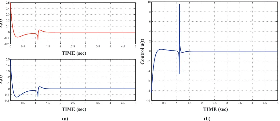
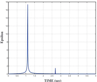
with initial conditions x(0) = [0.5,0.5]T . The aim is to set the closed-loop poles at σ = (−8,−6). When the pole placement method is applied, it can be seen in Figure 1.a that despite the poles being successfully allocated at the designed location, the shape of the response shows a jump along the time interval and so does the designed control u(t) = −K(t)x(t), (Figure 1.b). Plotting the profile of ǫ(h), it can be seen it reflects the two discontinuities at times t = 1.1 secs and t = 2.68 secs, where the condition for differentiability of P(t) fails (Figure 2.a). In Figure 2.b an estimate of the differentiability of P(t) is shown, it is represented by the quantity P(t+hh)−P(t) calculated at each step
h of the time interval. As expected it shows two discontinuities along the interval[0, tf], the first one happening at t = 1.1 sec and the second one at t = 2.68 sec. On the other hand, if now the location of the poles is shifted to be i.e. σ = (−12,−10), Figures 3.a and 3.b show the components of the response and the control law for this choice of left hand side poles.
This time it can be seen how the discontinuities in the stable responses and the control after the pole placement are smoother than in the previous case. The plot of epsilonǫ(h) in Figure 4 clearly shows two discontinuities too, verifying the existence of the relation between P(t), Λ(t), A(t), B(t) and
K(t) as indicated in (22). As the desired poles have changed, so did Λ(t)and consequently K(t)and
TIME (sec)
TIME (sec)
x
(t)1
x
(t)2
(a)
TIME (sec)
C
on
tr
olu(t)
(b)
Fig. 1: (a) Components of the responsex1(t), x2(t). The shape of the response shows a jump att= 1.1
seconds. (b) Control signal u(t) = −Kx(t) for the desired set of chosen poles σ = (−8,−6). The shape of u(t) shows a jump at t= 1.1 seconds
IV. GENERALIZATION TO NONLINEARSYSTEMS
In this section an approach to the problem of pole placement when the system under consideration is nonlinear is presented. A nonlinear system of the form:
˙
x=A(x)x(t) +B(x)u(t), x(0) =x0 (23)
where A(x) ∈Rnxn, B(x) ∈Rmxn, u(t) is the control signal and x(0) =x
0 is the vector containing
the given initial conditions. (23) can be written as a sequence of linear time-varying systems:
˙
x(1) =A(x0)x(1)(t) +B(x0)u(1)(t), x(1)(0) =x0
..
. (24)
˙
x(i) =A(x(i−1)
(t))x(i)(t) +B(x(i−1)
(t))u(i)(t), x(i)(0) =x
0
Applying the methodology presented in Section III, for some given choice of closed-loop poles, i.e.
σ = (λ1d,· · ·λnd), a sequence of feedback control laws of the form u(i)(t) = −K(i)(t)x(i)(t) is obtained at each iterationi, each K(i) is the feedback gain obtained to ensure stability on each of the
iterates closed-loop forms:
˙
x(1) = [A(x0(t))−B(x0(t))K(1)(t)]x(1)(t), x(1)(0) =x0
..
. (25)
˙
x(i) = [A(x(i−1)
(t))−B(x(i−1)
(t))K(i)(t)]x(i)(t), x(i)(0) =x
0
Now, the eigenvalue placement theorem can be applied to each of these systems (25) being the set of desired poles σ = (λ1d,· · ·λnd) chosen to be the same for each iteration:
det[λ·I−A(x0) +B(x0)K(1)(t)] = (λ−λ1d)· · ·(λ−λnd)
..
[image:8.595.65.520.60.258.2]TIME (sec)
E
psilo
n
(a)
TIME (sec)
D
iffer
en
tiab
ilityofP
(t)
(b)
Fig. 2: (a) ǫ(h) shows discontinuities at times t = 1.1 seconds and t = 2.68 seconds where the condition for differentiability of P(t) fails. (b) Differentiability of P(t) is lost at the same times where ǫ(h) is discontinuous.
det[λ·I−A(x(i−1)
(t)) +B(x(i−1)
(t))K(i)(t)] = (λ−λ
1d)· · ·(λ−λnd)
Therefore, each of these linear time-varying closed loop systems (25) will be exponentially stable provided the conditions from Section III-C are satisfied.
After a finite number of iterations, the solutionx(i)(t) converges to the nonlinear solutionx(t). Then,
the last iterated feedback gain K(i)(t) that stabilises the ”ith” system, can be applied to the original nonlinear system in order to satisfy the stability requirements for this nonlinear closed-loop:
˙
x= [A(x(t))−B(x(t))K(i)(t)]x(t), x(0) =x
0
provided that the desired eigenvalues σ = (λ1,· · ·λn) are chosen to be far on the left-half plane as stated in Section III-C.
The exponential stability of the nonlinear system achieved as indicated here can be summarized as follows: Given a nonlinear system of the form (23) where the matrices A(x) and B(x) are Lipschitz and the pair (A, B) is controllable ∀x(t),∀t∈[0, T], there exists a feedback control u(t) given by:
limi→∞u
(i)(t) =lim
i→∞K
(i)(t)x(t)→u(t)
whereK(i)(t)is Lipschitz, such that the solutionx(t)of the nonlinear system is exponentially stable in [0, T]. Proof: We need to assume thatK(i)(t)satisfies the Lipschitz condition at each iteration,
(differentiability is a necessary condition for exponential stability of the linear time-varying systems on the sequence) and also that A(x) and B(x) are Lipschitz, then, the iteration technique can be applied. By applying the pole placement algorithm, an algebraic equation is set and solved at each iteration in order to obtain the elements of the corresponding feedback gain matrix K(i)(t);
λn+ Γ(i)
n−1λ
n−1
+ Γ(ni−)2λ
n−2
+· · ·+ Γ(1i)λ1 +λ0 = (λ−λ1)(λ−λ2)· · ·(λ−λn) (27)
The coefficientsΓ(ji) are a linear combination of the linear elements of K(i)(t) =
h
k(1i)(t), . . . , k(i)
n (t)
i
[image:9.595.63.517.57.255.2]TIME (sec) TIME (sec)
x
(t
)
1
x
(t
)
2
(a)
TIME (sec)
C
on
tr
olu
(t)
(b)
Fig. 3: (a) Components of the responsex1(t), x2(t). The shape of the response shows a smoother jump than in the previous case. (b) Control u(t) =−Kx(t)when the poles of the close loop are shifted to
σ= (−12,−10).
TIME (sec)
E
p
silo
[image:10.595.62.520.61.260.2]n
Fig. 4: ǫ(h) shows two discontinuities. This verifies the existence of the relation between P(t), Λ(t),
A(t), B(t) and K(t) as indicated in (22)
In order to solve this, identification of parameters needs to be performed at this stage, simply by equating the coefficients on both sides of equation (27):
Γ(ni−)1 =α
(i)
n−1+β (i)
n−1·k (i)
n−1(t) = φn−1(λ1,· · · , λn)
Γ(ni−)2 =α
(i)
n−2+β (i)
n−2·k (i)
n−2(t) = φn−2(λ1,· · · , λn) ..
.
Γ(1i) =α
(i)
1 +β
(i) 1 ·k
(i)
1 (t) = φ1(λ1,· · · , λn)
(28)
Therefore, the elements of K(i)(t) of the feedback gain can be obtained by solving each of the
equations in (28):
kn(i−)1(t) =
φ(ni−)1(λ1,···,λn)−α(ni−)1
β(ni−)1
,· · · , k1(i)(t) =
φ(1i)(λ1,···,λn)−α(1i)
[image:10.595.188.385.333.501.2]The functionsα(i) andβ(i) at each iteration depend on those elements ofA(x(i−1)
(t))andB(x(i−1)
(t))
which are nonzero due to the pole placement, so that K(i)(t) is a Lipschitz function. Therefore,
provided that K(i)(t), A(x) and B(x) are Lipschitz functions, then by Theorem II, the sequence of
exponentially stable solutions of (25) converges to the exponentially stable solution of the original nonlinear problem.
V. APPLICATION TO F-8CRUSSADERAIRCRAFT
In this section this pole placement technique will be applied to the nonlinear equations of the F-8
aircraft in a level trim, unaccelerated flight at Mach=0.85 and altitude of 30.000 ft (9000m). The nonlinear equations are taken from ([William et al.(1977)]) and represent the dynamics of such an aircraft:
˙
x1 =−0.877x1+ 0.47x21+ 3.846x31−0.019x22−x3x21 −0.088x3x1−0.215u1(t)
˙
x2 =x3
˙
x3 =−4.208x1−0.47x21−3.564x31−0.396x3−20.967u3(t)
(30)
where x1(t) is the angle of attack (rad), x2(t) the pitch angle (rad),x3(t)the pitch rate (rad s−1
) and
u(t) = [u1(t), u2(t), u3(t)] is the control input vector.
The control objective in here is to place the desired poles of this nonlinear system on the left hand side of the complex plane by applying simultaneously the iteration technique and the placement algorithm introduced in Section 3 for linear time-varying plants.
The set of desired poles is σ =−10,−1.7108,−0.5129. This choice of poles corresponds to the closed-loop poles of the linearized and stabilized system when the control µ=−0.053x1 + 0.5x2+ 0.521x3 is applied (see [William et al.(1977)] for details).
The first step was to write in Matlab equation (30) in the form x˙(t) =A(x)x(t) +B(x)u(t), this is:
˙ x1 ˙ x2 ˙ x3 =
−0.877 + 0.47x1+ 3.846x21 −0.019x2 −x21−0.088x1
0 0 1
−4.208−0.47x1−3.564x21 0 −0.396
x1 x2 x3 +
−0.215 0 −20.967
u(t)
(31) and generate a sequence of 30linear time-varying systems:
˙
x(1)(t) =
α(1)11 α
(1)
12 α
(1) 13
0 0 1
α(1)31 0 −0.396
x
(1)(t) +B·u(1)(t)
.. .
˙
x(i)(t) =
α(11i) α
(i)
12 α
(i) 13
0 0 1
α(31i) 0 −0.396
x
TIME (sec)
TIME (sec)
TIME (sec)
Angleofattack
Pitchangle
Pitchrate
(a)
TIME (sec)
CONTROL
(b)
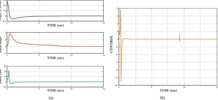
Fig. 5: (a) Closed Loop response. Statesx1(t), x2(t) and x3(t). (b) Control law u(t).
with
α(1)11 =−0.877 + 0.47x1(0) + 3.846x2
1(0), α
(1)
12 =−0.019x2,
α(1)13 =−x21(0)−0.088x1(0), α
(1)
31 =−4.208−0.47x1(0)−3.564x21(0),
α(11i)=−0.877 + 0.47x
(i−1)
1 + 3.846
x(1i−1)
2
, α(12i) =−0.019x
(i−1)
2 ,
α(13i)=−
x(i−1)
1 2
−0.088x(i−1)
1 , α
(i)
31 =−4.208−0.47x (i−1)
1 −3.564
x(i−1)
1 2
,
B = [−0.215,0,−20.967]T
where the initial conditions are x(0) = [x1(0), x2(0), x3(0)] = [0.5253,0,0]T. At each iteration ”i” a feedback law u(i)(t) =−K(i)(t)x(i)(t)is designed following the specifications: this is, the closed-loop
poles at each iteration should be allocated at λd=
−10,−1.7108,−0.5129,
˙
x(i)(t) =A(x(i−1)
(t))x(i)(t)−B(x(i−1)
(t))K(i)(t)x(i)(t) = ˜A(x(i−1)
(t))x(i)(t)
where A˜(x(i−1)
(t)) is the closed-loop matrix for the ith iteration. Using Ackerman′
s formula:
dethλ·I−A˜(x(i−1)
(t))i=λ−λ1
λ−λ2
λ−λ3
, (32)
in this way, a feedback matrixK(i−1)
(t)at each iteration is obtained. The simulations for each iteration were carried outtf = 15 sec with a time step of h= 0.01. After 30iterations, the sequence of linear time-varying systems converges to the nonlinear system; taking the30thfeedback control and applying this to the nonlinear system,
˙
x(t) =A(x)x(t)−B(x)K(30)(t)x(t)
it can be seen how the states of the nonlinear system converge to zero, Figure 5.a. The control law applied to the nonlinear system is shown in Figure 5.b, it presents an isolated discontinuity in the differentiability of the matrix of eigenvalues P(t); this does not affect the states as shown in Figure 5.a.
[image:12.595.65.517.56.264.2]is a non realistic scenario. In spite of this, both states reach exponential stability within the working time interval, this is the main purpose of this numerical example, to demonstrate convergence of the presented method and exponential stability achievement. The scenario in spite of being represented by a highly nonlinear equation is not intended to be a realistic one, in fact, the full set of equations of motion of a fighter aircraft is not 3-dimensional like in this case. Issues such as robustness, adequacy of the methodology, minimization of overshoot maximum value...etc, have not being dealt with as they are not under study in this work. All these issues are currently investigated by the authors and the findings will be presented in a future contribution.
VI. CONCLUSIONS
In this article a pole-placement algorithm for nonlinear systems has been presented. The method is based on the application of an iteration technique that replaces the nonlinear system by a sequence of linear time-varying systems.
Once this sequence of linear time-varying systems has been obtained, a standard pole-placement procedure is applied for each of the linear time-varying systems by dividing the interval in N steps of length h and applying Duhamel′
s principle. It has been shown how this method alone does not guarantee stability for linear time-varying systems and therefore additional requirements for stability were developed in Section 3:
If the matrices A(t), B(t), P(t) and K(t) are differentiable, then, writing equation (22) in the form:
˙Λ =P−1
(t)A˙(t)−B˙(t)K(t)−B(t) ˙K(t)P(t) + Λ(t)P−1
(t) ˙P(t)−P−1
(t) ˙P(t)Λ(t) (33)
gives a coupled equation relating P(t), K(t) and Λ(t) which states that these are not independent. Hence, in general, it may not be possible (in some cases) to choose Λ constant. Thus, equation (33) is an important condition for the exponential stability of the already pole placed linear time-varying system.
The restriction it places on P(t), K(t) and Λ(t) at the moment are the object of further research. These results were extended to nonlinear systems by the convergence of the iteration technique, thus the feedback gain designed for the last of the linear time-varying iterated systems is applied to the nonlinear system and achieving in this way exponential stability. Due to the accurate approach of the iteration technique to the original nonlinear plant, this pole placement method results in a more robust method than those relying on the linearization of the original system, at least the uncertainties of the unmodelled original dynamics do not exist in this case.
Some numerical examples were presented showing how the technique works and showing that, even in the case where differentiability of P(t) is not satisfied at every point of the time interval [0, t], the nonlinear system can be stabilized using this technique.
REFERENCES
[Ackermanet al.(1972)] Ackerman, J. (1972), Abtastregelung, Berlin/New York, Springer-Verlag, ISBN 0387057072.
[Aeyels et al.(1991)] Aeyels, D. and Willems, J.L. (1991), “Pole assignment for linear time-invariant second-order systems by periodic static output feedback.” IMA J. of Mathematical Control and Information, 8, 267-274.
[Aeyels et al.(1992)] Aeyels, D. and Willems, J.L., (1992), “Pole assignment for linear time-invariant systems by periodic memoryless output feedback.” Automatica, 28, 1159-1168.
[Bengtsson(1977)] Bengtsson, G. (1977), “Output regulations and internal models- a frequency domain approach.” Automatica, 13, 333-345.
[Choi(1995)] Choi, J. W., Lee, L. G., Kim, Y. and Kang, T. (1995), “Design of an effective controller via disturbance accomodating left eigenstructure assingment.” AIAA Journal of Guidance, Control and Dynamics, 18, 347-354.
[Choi(1996)] Choi, J. W., Lee, L. G., Suzuki, H. and Suzuki, T. (1996), “Comments on Matrix Method of Eigenstructure Assignment: The multi-input Case with application.” AIAA Journal of Guidance, Control and Dynamics, 19, 983.
[Choi(1998)] Choi, J.W. (1998), “Left eigenstructure assignment via the Sylvester equation.” KSME International Journal, 12, 1034-1040.
[Chow(1990)] Chow, J.H. (1990), “A Pole-Placement Design Approach for Systems with Multiple Operating Conditions.” IEEE
Transactions on Automatic Control, 35(3), 278-288.
[Francis et al.(1976)] Francis, B. A. and Wonham, W. M. (1976), “The internal model principle of control theory.” Automatica, 12, 457-465.
[Greschak et al.(1990)] Greschak, J. P. and Verghese, G.C. (1990), “Periodically varying compensation of time-invariant systems.”
Syst. Control Lett., 2, 88-93.
[Isidori(1989)] Isidori, A. (1989), Springer-Verlag, London., “Nonlinear Control Systems: An introduction.”
[Kailath(1980)] Kailath, T. (1980), “Linear Systems.” IEEE Trans. Autom. Control., XXI, 682, Prentice Hall, 12, Englewood Cliffs. [Kautsky et al.(1985)] Kautsky, J., Nichols N. K. and Van Doren P. (1985), “Robust pole assignment in linear state feedback.” Int. J.
Control, 41, 1129-1155.
[Kazantzis et al.(2000)] Kazantzis, N. and Costas, K. (2000), “Singular PDEs and the single step formulation of feedback linearization with pole placement.” Systems and Control letters, 39, 115–122.
[Luenberger(1967)] Luenberger, D. G. (1967), “Canonical forms for linear multivariable systems.” IEEE Trans. Autom. Control, 12, 290-292.
[Miminis(1982)] Miminis, G.S. and Paige, C.C. (1982), “An algorithm for pole assigment of time invariant linear systems.” Int. J. Control, 45(5), 341-354.
[Navarro-Hernandez et al.(2003)] Navarro-Hernandez, C. , Banks, S.P, and Aldeen, M. (2003). “Observer Design for Nonlinear Systems using Linear Approximations.” IMA J. Math. Cont Inf 20(3), 359-370. doi:10.1093/imamci/20.3.359
[Petkov et al.(1985)] Petkov, P.H. and Christov, N. D. and Konstantinov, M. M. (1985), “Computational algorithms for linear control systems: a brief review.” Int. J. Syst. Sci., 16, 465-477.
[Silverman(1966)] Silverman, L. M. (1966), “Transformation of time-variable systems to canonical (phase-variable) form.” IEEE
Trans. Autom. Control, 11, 300-303.
[Sontag(1998)] Sontang, E. (1998), Springer-Verlag, New York., “Mathematical Control Theory: Deterministic Finite Dimensional Systems.” 2ndEd.,
[Tayfun Cimen et al.(2004)] Tayfun Cimen and Stephen P. Banks, (2004).“Nonlinear optimal tracking control with application to super-tankers for autopilot design.” Automatica, 40, (11), 1845-1863.
[Tomas-Rodriguez et al.(2003)] Tomas-Rodriguez M. and Banks S.P., (2003). “Linear Approximations to Nonlinear Dynamical Systems with Applications to Stability and Spectral Theory.” IMA J. Math. Cont Inf., 20, 89-104.
[Tomas-Rodriguez et al.(2005)] Tomas-Rodriguez M., Navarro Hernandez C. and Banks S.P., (2005). “Parametric Approach to Optimal Nonlinear Control Problem using Orthogonal Expansions.” In proceedings of 16th IFAC World Congress, 16, 747, Prague, July 2005, Cz.
[Tomas-Rodriguez et al.(2010)] Tomas-Rodriguez M. and Banks S.P., (2010). “Linear, Time-varying Approximations to Nonlinear Dynamical Systems with Applications in Control and Optimization.” Lecture Notes in Control and Information Sciences, Vol. 400, XII, 298 p.
[Tuel(1967)] Tuel, W. G. (1967) , “On the transformation to (phase-variable) canonical form.” IEEE Trans. Autom. Control, 12, 607. [Varga(1981)] Varga, A. (1981), “A Schur method for pole assignment.” IEEE Trans. Autom. Control, 26, 517-519.
Automatica, 31(11), 1605-1617.
[Valasek et al.(1995b)] Valasek, M. and Olgac N. (1995), “An efficient pole placement technique for linear time invariant SI SO
systems.” IEEE Control Theory Applications. Proc. D 142(5), 451-458.
[Valasek et al.(1999)] Valasek, M. and Olgac N. (1999), “Pole placement for linear time-varying non-lexicographically fixedM I M O
systems.” Automatica, 35, 101-108.