An overview of the development of the hybrid method for seismic vulnerability assessment of buildings

City, University of London Institutional Repository

Citation

:

This is the accepted version of the paper.

This version of the publication may differ from the final published

version.

Permanent repository link:

Link to published version

:

Copyright and reuse:

City Research Online aims to make research

outputs of City, University of London available to a wider audience.

Copyright and Moral Rights remain with the author(s) and/or copyright

holders. URLs from City Research Online may be freely distributed and

linked to.

City Research Online: http://openaccess.city.ac.uk/ [email protected]

1

An overview of the development of the hybrid method for

seismic vulnerability assessment of buildings

Andreas J. Kappos

Research Centre for Civil Engineering Structures, City University London, UK

Northampton Sq., London EC1V 0HB; email: [email protected]

2

An overview of the development of the hybrid method for

seismic vulnerability assessment of buildings

The paper presents in a chronological and systematic way the development of the hybrid method for seismic vulnerability assessment of structures, which

combines use of empirical databases of earthquake damage with the results of nonlinear analysis of representative structural models. The key concepts and milestones in the development of the method are identified, and selected

examples of its application are summarised. The first part of the paper focuses on the derivation of hybrid damage probability matrices and the second one with the derivation of fragility curves for reinforced concrete and masonry buildings. Finally some general conclusions are drawn and directions of future research on the hybrid approach are suggested.

Keywords: seismic vulnerability; hybrid methodology; fragility curves; loss assessment; reinforced concrete buildings; masonry buildings

Introduction

Methodologies for assessing the seismic vulnerability of a large number of structures (as opposed to that of a specific structure), like building stocks in urban centres, have emerged in the 1970’s; arguably the best-known pertinent work from that era was that of Whitman et al. (1973) on the derivation of Damage Probability Matrices (DPMs). Initially confined mainly in conference proceedings, due to the concern of the authors, and arguably also of the reviewers of journal papers, resulting from the several

3

The most common tools for seismic vulnerability assessment of populations of structures are

• DPMs, i.e. matrices indicating the degree of damage caused to a certain structural type (e.g. low-rise stone masonry buildings) for a given earthquake intensity, expressed either in terms of macroseismic intensity (I) or peak ground acceleration (PGA), and

• Fragility curves, i.e. probabilistic vulnerability curves, typically representing the probability of exceeding a certain damage state (DS) for a given earthquake intensity. Adopting the lognormal cumulative density function, as commonly done in seismic fragility studies, and selecting PGA as the intensity parameter, the curve is given by

1

P[ | ]=Φ[ ln( )]

β ≥

i

i ,ds

i

ds PGA

PGA

ds ds PGA (1)

where

i

ds

PGA, is the median value of peak ground acceleration at which the building reaches

the threshold of damage state, dsi

βdsi is the standard deviation of the natural logarithm of peak ground acceleration for

damage state dsi

Φ is the standard normal cumulative distribution function.

In addition to the rigorous (probabilistic) fragility curves, there is an abundance of ‘non-probabilistic’ vulnerability curves in the literature, such as those indicating the evolution of damage as earthquake intensity increases, for which the author has

introduced in 2006 the term ‘primary vulnerability curve’, as well as several functions of the so-called ‘vulnerability index’ (see Calvi et al. 2006).

The methodologies for deriving the above matrices or functions can be broadly classified as

• empirical, based on statistical data of damage in past earthquakes

• analytical, based on analysis of representative models of each structural class

4

This paper focuses on the third approach that has been developed (in the context of seismic vulnerability assessment) primarily by the author and a number of

co-workers (see Acknowledgements). The basic reason for developing this approach has been the long-recognised fact that there is an abundance of statistical data for seismic damage in the intensity range from VI to VIII and a lack of data in the other intensities. It is perhaps worth noting that the stimulus for writing this paper was that the hybrid approach, while well-known as a concept, is still not well-known in its details and is often referenced/cited in an incomplete or even incorrect way. Hence the main objective of this article is to gather together the basic concepts of the method, identify the main challenges and developments, and provide the most recent examples from its

application. All important aspects of the method are presented (using terminology adjusted to the current international trends) in sufficient detail for the reader to appreciate them without having to make recourse to the original papers; this decision led to limiting this presentation to the studies by the author and his co-workers, leaving beyond its scope a few studies by other authors that also entail some elements of the hybrid approach, that by Barbat et al. 1996, constituting the earlier and more interesting among those.

Early developments – the hybrid approach to derivation of DPMs

5

numerous limitations involved in both the derivation of the input accelerograms and the nonlinear analysis of the 2D structures, they decided to combine analysis and damage statistics from the M6.5 earthquake and estimate future damage using the relationship

Ca(7.0) = Ca(6.5)⋅Cc(7.0)/Cc(6.5) (2)

where Ca is the actual cost of repair (from the statistical database) and Cc the value calculated using the analytical models. This is indeed the most rudimentary hybrid approach, i.e. using the analysis results for scaling the empirical (statistical) repair cost data, assuming the latter is reliable in absolute terms, whereas analytical data is reliable in relative terms.

Analytical estimation of economic loss

A key requirement in the hybrid approach is expressing empirical and analytical data in a uniform way, for which there is no obvious best choice. The approach used by Kappos et al. (1991) originated from the fact that damage statistics was available not only in the usual way of post-earthquake tagging, i.e. green-yellow-red tags, broadly corresponding to light-medium-heavy damage, but also in terms of cost of ‘repair’, which actually refers to all types of structural interventions used that included strengthening in several cases (notably when R/C jacketing was used in buildings with significant damage). It is worth noting that the database of 1978 earthquake damage for Thessaloniki remains the most comprehensive one in Greece in terms of both the extent of the area covered and the number of data collected from the files of the intervention studies that followed the 1978 earthquake, despite the fact that an effort to gather similar data was also made in a number of more recent earthquakes, such as the 1999 Athens earthquake (e.g. Kappos et al. 2007).

6

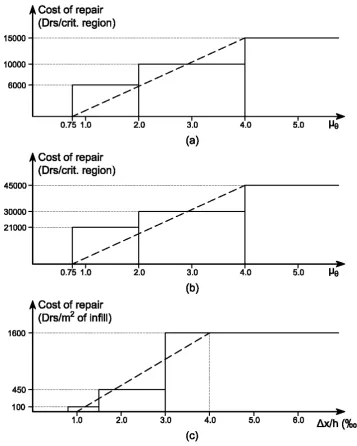
infills), as estimated by the Aristotle University group, based on their experience with the repair-strengthening techniques used after the Thessaloniki earthquake. For R/C members the first step corresponds to an actual intervention type, i.e. use of epoxy resin to seal cracks (a typical repair technique), the second step corresponds to bonding of metal plates on the damaged faces, and the third step to the construction of an R/C jacket around the damaged region, or part of it, as in the case of beams. For brick masonry walls, the three steps correspond to replastering the region with cracks, use of wire fabric along the main cracks, and demolition and reconstruction. Clearly, there is substantial uncertainty in establishing the thresholds of ductility μθ or drift Δx/h for

each intervention, hence the models shown in dashed lines in Fig. 1, which are

continuous rather than stepwise, lead to more reasonable results and were actually used in the aforementioned study.

Starting from the models shown in Fig. 1, Kappos et al. (1998) proposed

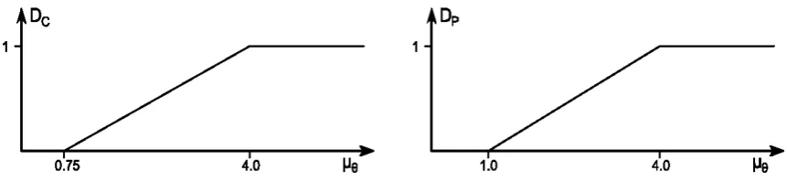
normalised versions, wherein for R/C members the cost is normalised to that of the most expensive intervention, typically, though not necessarily, jacketing, and is calculated as a function of the largest rotational ductility ratio in the member, whereas for brick masonry infills the cost is normalised to that of replacing the infill and is calculated as a function of the interstorey drift at the storey where the infill is located. Hence, referring to Figure 2, the economic damage index for an R/C member Dc is equal to 1 when jacketing is used, and less than 1 when other techniques (shotcreting, injection of resins, gluing of metal plates) are used.

For the loss index to be calculated for the entire building, a weighting factor wi is defined for each critical region i as the ratio of concrete volume in the region to the total volume of all concrete members (beams, columns, walls). If the total number of

R/C members is N, then w_i i N =



1, since each critical region is deemed to extend half a

member length.

The global economic damage index for the entire R/C structural system is

7

and its max value Dcg = 1 corresponds to the case wherein all structural members are strengthened using the most costly technique (μθ ≥4 in all R/C members). If the total cost of these interventions is Cc and the total value of the building, including structural and non-structural elements, as well as all installations, is Ctot, then the economic intervention index for the entire R/C structural system is defined as

G D C

C c cg c

tot

= ⋅ (4)

and expresses the cost of intervention as a fraction of the total cost of the building. Bearing in mind that the value of an existing building, having an age Tn years, is not the same as that of a similar new building (for which Ctot can be readily evaluated from current market rates), the cost can be estimated as

C T

T C

tot n rem d tot , = ,       γ 0 (5)

where Td is the design life of the structure and Trem = Td −Tn its “remaining” life after n

years. Based on data from Greek practice, Td = 67 yrs. and γ = 1 may be assumed, corresponding to an annual depreciation of 1.5%.

A (structural damage) vs. (loss) correlation model similar to the one used for R/C members is proposed by Kappos et al. (1998) for masonry infill wall panels (Fig. 2-right). In this case loss is correlated to the interstorey drift ratio, and the intervention types are different from those used for R/C members; in the case of masonry infills the most costly repair consists in demolition of the existing panel and construction of a new one. The intervention index for the infill panels is then defined as

G D C

C p pg

p

tot

= ⋅ (6)

where the global economic damage index Dpg is defined similarly to Dcg in equation (3)

and Cp is the total cost of replacing all infill panels in the building.

The global damage indices Dcg and Dpg can to be related to the global

8

R/C buildings with dual structural system (frames and walls), which is the most common type of medium and high rise R/C structure in Greece and Southern Europe, the empirical relationships (7) and (8) were proposed by Kappos et al. (1998);

appropriate adjustments are clearly required in countries where economic parameters are significantly different.

• For medium-rise structures (3-5 storeys):

G = Gc + Gp = 0.25Dcg + 0.08Dpg (7)

• For high-rise structures (8-10 storeys):

G = Gc + Gp = 0.30Dcg + 0.08Dpg (8)

Based on equations (7) and (8), if a building has suffered repairable damage, the required cost of interventions does not exceed 38% of the value of a similar new building; hence repair/strengthening, rather than reconstruction should be the optimum solution for all structures with a remaining life of 25 or more years (see equation 5). However, it is noted that the analysis used for deriving equations (7) and (8) did not account for repair of slabs and/or foundations; hence, in cases of heavy global damage (say G>0.25) slabs and foundations will probably have to be repaired, and the equations should be adjusted accordingly.

Derivation of DPMs using nonlinear dynamic analysis

The first application of the hybrid approach to vulnerability assessment of building stocks was made by Kappos et al. (1995) to derive DPMs for R/C buildings in Greece, using the data from the database of the 1978 earthquake damage (Penelis et al. 1989) and nonlinear response-history analysis of 2D models of representative low-rise (1-3 storeys), medium-rise (4-7 storeys), and high-rise (8-10 storeys) R/C buildings designed according to the provisions of the 1950s to 1970s codes, i.e. without any specific

9

and the other columns by appropriately scaling the aforementioned data on the basis of cost estimated as described in the previous section using the structural damage indices (ductility factors, drifts) calculated from response-history analysis. The assumption was made that all buildings in the studied part of the city fell within the same intensity zone, estimated as VII (MMI). It is now recognised that neither part of this assumption is strictly correct, i.e. the intensity was not really uniform in the study area (eastern Thessaloniki), and VII, albeit a reasonable value for a small area in the city centre where a collapse of a multi-storey R/C building occurred, is an overestimation of the average intensity in the area. Moreover, different groupings for buildings resting on "good" or "poor" soil were initially carried out, but since no conclusive trends with regard to the effect of soil conditions were detected, when the above mentioned methodology was applied, it was finally decided to construct a single DPM for each building class.

The columns of the DPMs referring to intensity VIII were estimated on the basis of analytical studies involving models of medium and high rise R/C buildings designed to the 1959 Seismic Code of Greece, which was in force up to 1984. Details of the design of buildings and a discussion of the limitations of the analytical models used may be found in Kappos et al. (1991). The models were first analysed for a total of 10 input motions, each corresponding to a typical soil profile in the area under

10

not increase linearly with intensity (e.g. Kappos 1997), the values suggested by ATC-13 (1985) were adopted; it is noted that the key objective of the Kappos et al. (1995) study was to derive benefit/cost ratios for pre-earthquake strengthening of buildings and the columns of the DPMs corresponding to intensities IX or higher contributed only marginally to the final ratios.

A more complete version of the hybrid method for deriving DPMs is reported in the paper by Kappos et al. (1998), which is often cited as the initial reference for the hybrid approach, although this is not really the case, as should be obvious from the foregoing paragraphs. In fact, as far as DPMs are concerned, the key improvement with respect to the previously described procedure is the use of the normalised models for correlating damage to cost of intervention shown in Fig. 2 in lieu of the initial ones of Fig. 1, the former in parallel with equations (7) and (8) to analytically estimate cost. Each row in the first column in Table 1 corresponds to one of the damage states (DS) considered (6 DS plus the undamaged state) which are the same as those adopted by ATC (1985); this has the double advantage of allowing meaningful comparisons with DPMs for US buildings and using the ATC-13 data for the very high intensities for which the hybrid method (as applied at that time) was not expected to produce reliable results. All DS are defined in terms of the central damage ratio, which can best be expressed as the cost of required (due to the damage induced) interventions to the replacement cost. The remaining columns include the percentage of medium-rise non-ductile R/C frames with brick masonry infills that fall within each DS for each

earthquake intensity (IMM). The last row can be seen as a condensed form of the DPM showing the average cost of damage at each intensity. The 4.8% shown for IMM=VII is the actual cost of damage for the specific category of buildings struck by the 1978 earthquake; the other columns were derived as described previously. It is noted that the economic damage indices calculated for intensity VII were reasonably close to those from the Thessaloniki 1978 data when the entire building stock was considered, but discrepancies for some individual building classes did exist.

Table 1. Damage probability matrix for medium-rise (4–7 storey) non-ductile R/C frames (Kappos et al. (1998).

Central damage ratio (%)

Modified Mercalli intensity

VI VII VIII IX X XI XII

11

0.5 45.0 40.9 34.8 0 0 0 0

5.0 15.3 19.3 24.3 1.9 0.2 0 0

20.0 10.0 10.9 11.5 65.1 30.8 3.6 0.5

45.0 0.6 1.2 4.3 33.0 67.7 70.0 27.9

80.0 0 1.2 1.4 0 1.3 26.4 71.2

100.0 0 0 0 0 0 0 0.4

Mean damage ratio 3.2 4.8 6.7 27.9 37.7 53.3 70.0

The same procedure was later used by Kappos et al. (2002) to derive DPMs for the building stock of another city in Greece (Volos). It is worth noting that during the course of that project it was found out that damage data collected in Greece after earthquakes more recent than the 1978 one (Kalamata 1986, Pirgos 1993, Patras 1993, Aegion 1995), albeit valuable, were generally not in a form that economic damage statistics could be reliably assessed for a representative set of buildings. What usually happened was that the collected data concerned only buildings that were inspected for a second time and/or wherein some post-earthquake intervention had taken place;

furthermore, the extent of the geographical area, hence the total building stock to which the data refers, was often unclear. Since no empirical data was available for Volos, the Thessaloniki database was used, while the analytical part of the hybrid procedure was carried out using a different set of ground motions, i.e. 16 accelerograms that

represented the scenario earthquake motion in each sub-zone of the city. The 16 accelerograms were scaled, using the previously discussed procedure, to match four different intensities (VI to IX), so that average values of the economic damage indices could be estimated for each building type for all these intensities (that were the critical ones).

12

most appropriate values using the resulting shape of the fragility curve (see next section) as the main criterion. This empirical correction only affects the two lowest damage states in the DPMs (see Table 1), if the ‘no damage’ state is kept separate from the ‘slight damage’ state (cost ratio <1%), which is important for low intensities, but increasingly less so for higher intensities. Engineering judgement can be used in

combination with available data to assign reasonable percentages of buildings to each of the two lowest damage states, or appropriate curve fitting of the corresponding

multilinear fragility curve can be made, e.g. using a lognormal distribution function, and then the DPM be accordingly revised.

Damage probability matrices were derived (Kappos et al. 2002b) for the following 18 R/C building typologies:

• “Old” dual R/C systems (wall+frames) regularly infilled with masonry walls, 1-3 storeys

• “Old” dual R/C systems irregularly infilled with masonry walls (pilotis), 1-3 storeys

• “Old” dual R/C systems without infills, 1-3 storeys

• “Old” dual R/C systems regularly infilled with masonry walls, 4-7 storeys

• “Old” dual R/C systems irregularly infilled with masonry walls (pilotis), 4-7 storeys

• “Old” dual R/C systems without infills, 4-7 storeys

• “Old” dual R/C systems regularly infilled with masonry walls, ≥ 8 storeys

• “Old” dual R/C systems irregularly infilled with masonry walls (pilotis), ≥ 8 storeys

• “Old” dual R/C systems without infills, ≥ 8 storeys

• The above 9 types of structures, but designed to modern code(post-1990) provisions.

DPMs for new buildings, built in the 1990s and beyond, were derived by a double scaling of the empirical data available for ‘old’ buildings using analytical results calculated for new buildings, i.e. one scaling factor was the ratio of analytically derived cost of intervention for a particular building type designed to the two procedures

13

Derivation of DPMs using nonlinear static analysis

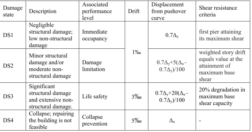
The type of analysis to be used in the hybrid approach is also a major consideration. In the case of unreinforced masonry (URM) buildings use of nonlinear response-history analysis is cumbersome if realistic structures are to be analysed for a large number of ground motions, as is the case with vulnerability assessment. Hence the AUTh group, along with several others, have long been using nonlinear static (‘pushover’) analysis for assessing the seismic response of URM structures. Most of these analyses have been carried out using the equivalent frame model (Kappos et al. 2002a), which renders nonlinear analysis feasible even for large 3D structures. When pushover curves, better called ‘resistance curves’, i.e. plots of base shear vs. top displacement, are derived from this analysis, global damage indices can be conveniently estimated without the need to start from local damage (such as Dci in equation 3). As first suggested by Kappos (2001), DS can be defined in terms of selected values of top displacement, typically fractions of the yield displacement Δy and the displacement at failure Δu. Table 2 summarises the most important proposals for the definition of damage state for URM buildings; the 5th _{column includes the aforementioned thresholds in terms of top}

displacement, while other columns present alternative definitions in terms of interstorey drift or base shear.

Table 2. Damage state definitions for masonry buildings (Kappos & Papanikolaou 2015).

Damage

state Description

Associated performance

level Drift

Displacement from pushover curve Shear resistance criteria DS1 Negligible structural damage; low non-structural damage Immediate occupancy 1‰

0.7Δy first pier attaining _{its maximum shear}

DS2 Minor structural damage and/or moderate non-structural damage Damage

limitation 0.7Δy+5(Δu

-

0.7Δy)/100

weighted story drift equals value at the attainment of maximum base shear DS3 Significant structural damage and extensive non-structural damage.

Life safety 3‰ 0.7_0.7Δy_Δ+20(Δu-

y)/100

20% degradation in maximum base shear capacity

DS4 Collapse; repairing the building is not feasible

Collapse

14

Whereas deriving analytically DPMs and/or fragility curves using pushover analysis and the definitions of Table 2 is fairly straightforward, use of the hybrid approach is much more cumbersome in this case, as well as subject to substantial uncertainty. The AUTh group (Penelis et al. 2002) has utilised the two then available databases for seismic damage to URM buildings, the aforementioned one including the 1978 Thessaloniki earthquake data, and the one including the 1995 Aegion earthquake data, compiled by the University of Patras group; the assumption was made that the former corresponds to an intensity VII, while the latter to VIII. Rather than working with intensities, DPMs for URM buildings were derived in terms of spectral

displacement Sd, as also done in HAZUS (FEMA 2005) for fragility curves, which makes easier scaling on the basis of pushover analysis that predicts top displacement that can be easily related to Sd if a proper displacement spectrum is adopted and the concept of the equivalent SDOF system is invoked. This decision led to the need for a further crude assumption, i.e. that the representative Sd spectrum in each city was the one of the (only) available recorded ground motion. The DPMs corresponding to spectral displacements smaller than those from the Thessaloniki event were calculated by scaling down the Thessaloniki database, while the ones that correspond to higher than the Aegion event were calculated by scaling up the Aegion database. The scale factor was calculated by using the purely analytical DPMs for all spectral

displacements. It is clear that such a procedure, albeit interesting, is also subject to high uncertainty, primarily in the definition of the representative ground motion, but also in the analysis of the representative buildings and the definition of global damage states.

The hybrid approach to derivation of fragility curves

15

ratio is used for each curve, which is the average of the range of economic damage index values for the pertinent DS, e.g. 0.5% is the central value for DS1 which starts when damage exceeds 0 and ends at a damage equal to 1% the replacement cost of the building. Essentially, the multilinear segments of Fig. 3 are just a visual representation of a DPM and using them offers no real advantage over using the corresponding DPMs, except perhaps for calibrating the scaling procedure of zero (statistical) values of Ca, as discussed previously. Of course, cumulative density functions can be fitted to these segments, but even so the resulting curves will not be fragility curves in their standard form, i.e. each curve corresponding to the threshold of the pertinent DS. In fact the proper procedure, described in the remainder of this section, is exactly the opposite, i.e. first derive the fragility curve sets and then (whenever needed) the corresponding DPMs.

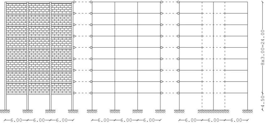
A rigorous procedure for deriving fragility curves for R/C buildings using the hybrid approach was presented by Kappos et al. (2004); the curves were derived in terms of PGA for a total of 5 DS (plus the undamaged one), essentially the same as those indicated in Table 2 but with the last DS split into DS4 and DS5. The statistical data set is the previously described one from the 1978 Thessaloniki earthquake. Nonlinear response history analysis was carried out for 2D models of the concrete buildings, either bare or with brick masonry infills; in the example shown in Fig. 4 the infills are discontinued at the ground storey (‘pilotis’ system), hence creating a soft storey effect. Response history analysis was carried out using the lumped plasticity models of DRAIN-2D 90 (Kappos & Dymiotis 2000). The input motions used were 16 accelerograms, 8 natural and 8 synthetic, representative of typical ground motions in Greece (see Kappos et al. 2006), and they were scaled to increasingly higher PGA values until failure criteria for the buildings were met. Performing successive response history analyses is currently known as incremental dynamic analysis (Vamvatsikos & Cornell 2002) but it is worth noting, since this is a historical review, that the basic concept of this approach, i.e. estimating the evolution of a demand parameter with increasing earthquake intensity, has been used by the author since the late 1980s (Kappos 1990).

16

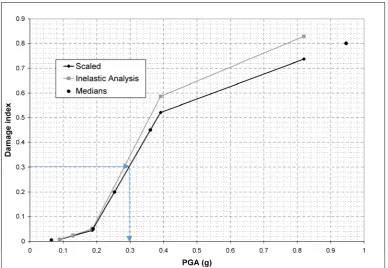
the primary vulnerability curve, i.e. the relationship describing the evolution of damage index (here the loss index L, i.e. the ratio of intervention to replacement cost) versus the earthquake intensity (here the PGA to which the ground motions are scaled); a typical example is shown in Figure 5 (grey line). Due to the fact that the cost of the R/C structural system and the infills totals less than 40% of the cost of a building, equations 7 and 8 give values up to 38% for the loss index L, wherein replacement cost refers to the entire building, including finishings, equipment etc. In the absence of a more exact model, situations leading to the need for replacement (rather than repair/strengthening) of the building were identified using analytical failure criteria for members and/or storeys (Kappos et al. 2006):

 In R/C frame structures, failure was assumed to occur (hence L=1) at the step where either 50% or more of the columns in a storey ‘failed’, i.e. their plastic rotation capacity was less than the corresponding demand calculated from the inelastic analysis, or the interstorey drift exceeded a value of 4% at any storey.

 In R/C dual structures, failure was assumed to occur (hence L=1) whenever either 50% or more of the columns in a storey ‘failed’, or the walls (which carry most of the lateral load) in a storey failed, or the interstorey drift exceeded a value of 2% at any storey (drifts at failure are substantially lower in systems with R/C walls).

Since the statistical database also includes the economic damage index, statistical values can be plotted on diagrams such as that of Fig. 5, provided the

corresponding intensity is expressed in the same way, here in terms of PGA. This can be easily done if PGA values in the damaged area are known, but often, especially for earthquakes that occurred in the last century, only macroseismic intensity (I) is

available. Of course, I can always be converted to PGA but it is well-known that this is associated with substantial scatter. In the studies by Kappos et al. (2004, 2006) the empirical relationship

ln(PGA)=0.74·I+0.03 (9)

suggested by Koliopoulos et al. (1998) was used; this equation is calibrated for

17

only, the intensity of the 1978 Thessaloniki earthquake in this case, the procedure is straightforward but subject to substantial uncertainty; if data for more intensities exists a more rigorous procedure can be followed (see next section).

Adopting the usual in seismic fragility analysis assumption of a lognormal distribution (equation 1), only two parameters are needed for each DS (i), the threshold

i

ds

PGA, (the median value of peak ground acceleration at which the building reaches

the DS) and the logarithmic standard deviation βdsi. The threshold PGA values are

readily obtained from the hybrid primary vulnerability curve (black line in Fig. 5) as soon as threshold values of economic damage index are defined for each DS; for instance, if DS4 starts for a loss index of 30% the corresponding PGA threshold for the building of Fig. 5 is about 0.3g.

Lognormal standard deviation values (β) describe the total variability associated with each fragility curve, which is mainly due to three sources: the definition of the damage states in terms of damage/loss indices, the uncertainties in defining the capacity of each structural type, and finally the variability of the demand imposed on the

structure by the earthquake ground motion. In the studies by Kappos et al. (2004, 2006) the uncertainty in the definition of damage state, for all building types and all damage states, was assumed to be β=0.4 (FEMA, 2005), the variability of the capacity for low-code buildings was assumed to be β=0.3 and for high-code β=0.25 (FEMA 2005), while the uncertainty in the seismic demand, was taken into consideration through a

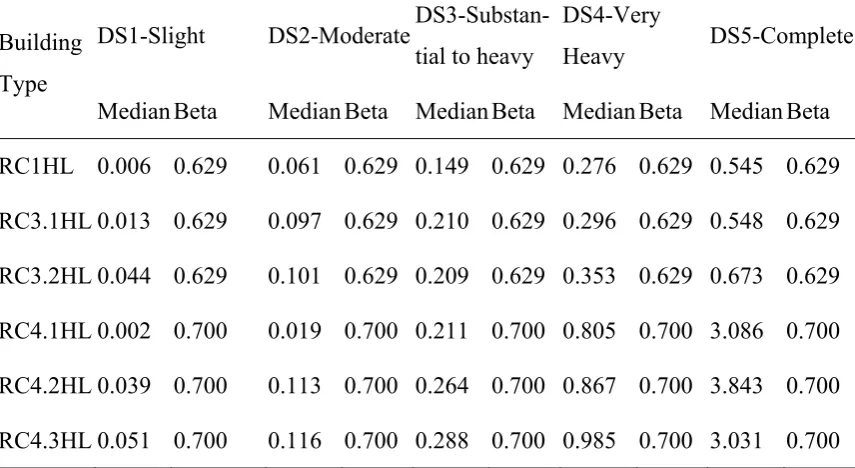
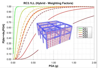
convolution procedure, i.e. by calculating the variability in the final results of inelastic dynamic analyses carried out for a total of 16 motions at each level of PGA considered. An example of median values (DS thresholds) and standard deviations is given in Table 3; RC1 are bare frames, RC3 are infilled frames (3.1 regularly infilled, 3.2 pilotis) and RC4 are dual systems (4.1 bare, 4.2 regularly infilled, 4.3 pilotis); see details of the classification scheme in Kappos et al, (2006).

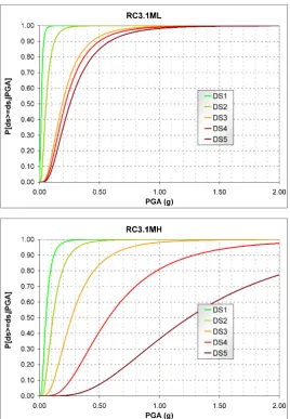
Figure 6 shows the finally resulting fragility curve sets for a typical case

18

Table 3. Estimated fragility curve parameters (median values of PGA in g), for R/C High-rise Buildings, Low-Code Design (Kappos et al. 2006).

Building Type

DS1-Slight DS2-Moderate DS3-Substan-tial to heavy

DS4-Very

Heavy DS5-Complete

Median Beta Median Beta Median Beta Median Beta Median Beta

RC1HL 0.006 0.629 0.061 0.629 0.149 0.629 0.276 0.629 0.545 0.629

RC3.1HL 0.013 0.629 0.097 0.629 0.210 0.629 0.296 0.629 0.548 0.629

RC3.2HL 0.044 0.629 0.101 0.629 0.209 0.629 0.353 0.629 0.673 0.629

RC4.1HL 0.002 0.700 0.019 0.700 0.211 0.700 0.805 0.700 3.086 0.700

RC4.2HL 0.039 0.700 0.113 0.700 0.264 0.700 0.867 0.700 3.843 0.700

RC4.3HL 0.051 0.700 0.116 0.700 0.288 0.700 0.985 0.700 3.031 0.700

In the paper by Kappos et al. (2006) an alternative representation of fragility curves is also presented, in terms of spectral displacement Sd. The procedure adopted for R/C buildings was to transform the median PGA values to corresponding median Sd values, using an appropriate spectrum and either the fundamental period of the

‘prototype’ building, assuming that the equal displacement rule applies, or using the capacity spectrum approach for short period buildings. For URM buildings, which are also addressed in that paper published in the special issue devoted to the results of the EU-funded project RISK-UE, fragility curves for URM buildings were derived using the displacement-based approach and the definitions based on fractions of Δy and Δu (Table 2), as described in the previous section. It is recalled that the Sd-based procedure is sensitive to the type of ‘representative’ response spectra selected for each earthquake intensity.

Latest developments in the hybrid approach for fragility analysis

19

presented in this section; the versions described herein represent the current state-of-the-art in the hybrid approach for fragility analysis.

A major limitation of the older versions of the hybrid approach was that they assumed that the actual damage statistics from previous earthquakes are reliable, whereas the analytical predictions of damage are reliable only in a relative way, hence they are basically used for scaling the former. This is, of course, not true when the statistical sample is insufficient, which is quite often the case, particularly when a rather detailed classification scheme is adopted. It is noted that in the RISK-UE classification a total of 54 classes were defined for R/C buildings (Kappos et al. 2006) since structural system, height, and level of seismic design were all taken into account. For several of these classes the number of buildings for which loss data was available was insufficient for reliable statistical processing in the Thessaloniki 1978 database; in fact, there is arguably no available database that includes sufficient data for all 54 classes. For such cases, different interpretations of the data were put forward by Kappos & Panagopoulos (2010), using the ratio λ =Lact/Lanl for I=6.5 which is the value associated with the

Thessaloniki earthquake database, after a re-evaluation of this intensity. Lact is the

‘actual’ (statistical) cost of damage and Lanl is the analytically calculated loss value

using nonlinear response-history analysis as discussed in the previous sections; note that L is the same as G in equations 7 and 8.

1. For building classes with sufficient statistical data the ratio λ is estimated as in the ‘standard’ hybrid approach. If statistical data is limited, then the λ value of the closer class with sufficient available data is used (e.g. RC3.2LL and RC3.1LL).

2. A common λ ratio for all building classes of the same height is used, defined as

, 6.5 , 6.5 1 1 λ = = = = =





3. The λ ratio is defined as in the 1st _{approach but a common loss index} anl I, 6.5=

aver

L (at

20

,

, 6.5 1

1 ( ) Ι= = = ⋅ =





L is the ‘actual’ (statistical) loss value at a point I=6.5 for building class i

,

anl I=6.5 i

L is the analytically calculated loss value at a point I=6.5 for building class i

i=1,2,...n building classes with sufficient available statistical data

Ni is the number of buildings assigned to class i in the database

The above three approaches were applied to the ‘low’ code building classes, since no ‘moderate’ or ‘high’ code buildings were present at the time the Thessaloniki 1978 earthquake occurred. The same λ ratios estimated for the ‘low’ code building classes were used for the corresponding (i.e. having the same structural system, height, infills arrangement) ‘moderate’ and ‘high’ code classes; e.g. λRC3.1ML= λRC3.1MM=

λRC3.1MH. Kappos & Panagopoulos (2010) found that the effect of the way statistical data

is interpreted in the hybrid approach on the resulting fragility curves was rather significant, particularly for the higher damage states.

Hybrid fragility curves based on statistical data for multiple intensities

21

of data for a single intensity, in lieu of the somewhat arbitrary ‘interpretations’ presented in the previous section.

Having established analytically the loss index L, the final value to be used for each PGA in the fragility analysis depends on whether an empirical value is available for that PGA or not, i.e.

(i) if the ‘actual’ (statistical-empirical) loss value at a point i (PGA=PGAi), Lact,i is

available in the database, the final value to be used is

Lfin,i = w1,iLact,i + w2,iLanl,i (w1,i+w2,i=1) (12)

where Lanl,i is the analytically calculated loss value for that PGAi and w1,i, w2,i are

weighting factors that depend on the sample size and the reliability of the empirical data available at that intensity. If Lact,i is based on more than about 60 buildings with reliable

data, w1,i equal to about 1 is recommended, if it is based on 6 buildings or less, w1,i

should be taken as zero (or nearly so). The ratio λi,=Lfin,i/Lanl,i at point i is

λi = w1,i(Lact,i /Lanl,i) + w2,i (13)

(ii) if the ‘actual’ loss value at a point j (PGAj), Lact,j is not available in the database,

new ‘actual’ loss values, as well as new weighting factors, are estimated using linear interpolation between points i and k corresponding to intensities for which data is available (PGAi<PGAj<PGAk).

Clearly, this is an interpolation scheme that aims to account in a feasible way for the strongly nonlinear relationship between intensity and damage-loss. In the common case that Lact is available at one or very few points the scheme should be properly

adapted, as discussed subsequently.

22

non-conservative fragility curves according to the procedure of the previous section, is observed for building classes with λ ratios significantly smaller than 1.0. The weighted hybrid approach manages to overcome these problems, provided that sufficient

statistical data is available for high (I≥8.0) intensity values.

Ground motion dependence of fragility curves

It should be clear from the discussions presented so far that the type of ground motion selected for carrying out the fragility analysis using the hybrid approach is always important. Hence, the question to be addressed is: Is it possible to adapt the fragility curves derived using a certain set of ground motions, generally compatible with a selected response spectrum, for them to be used in another area where the representative response spectrum is different? The question is far from purely academic, as loss

scenarios are often carried out for different parts of a country, or even for other

countries, using exactly the same fragility curves for the same building classes. One of the milestones in the development of the hybrid approach was the method proposed by Kappos et al. (2010), for carrying out this adaptation of fragility curves in a relatively low-cost way, i.e. avoiding to repeat the cumbersome analytical part for a different set of input motions. The adaptation of the fragility curves is carried out by scaling their damage state thresholds to match the intensity of the representative spectrum in the area under consideration, as described in the following.

It has long been recognised that the pseudo-velocity spectrum is a much better indicator of the destructiveness of an earthquake than the pseudo-acceleration spectrum commonly used for design. Hence the damage state thresholds of the hybrid fragility curves derived for a certain area are scaled using a uniform correction factor c,

calculated from the ratio of the area enclosed under each pseudo-velocity spectrum (Spv)

for a selected period range (e.g. from 0.1 to 2.0 sec) as follows:

c = Ehfc/ Erepr (14)

where Ehfc and Erepr denote the area under the mean pseudo-velocity spectrum of the

records used for the derivation of the hybrid fragility curves and the representative Spv

23

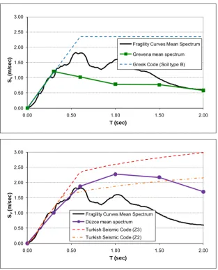
synthetic accelerograms representative of typical ground motions in Greece to two specific areas, one in Greece (Grevena) and one in Turkey (Düzce). The representative Spv spectra for each city, along with the spectra used for deriving the fragility curves are

shown in Fig. 8, and it is clear that in one case the former is clearly less destructive than the latter, whereas the opposite holds for the other city. As an example, using Eq. 14, a value c =1.38 was calculated for Grevena and was then used for the modification of all damage state medians in the R/C fragility curves, regardless of the building class they referred to.

This simple approach is quite general and very convenient for deriving site-specific analytical fragility curves for a building stock in a site-specific area, regardless of whether the appropriate ‘target’ spectrum is defined from a microzonation study or a seismic code. Alternatively, a more refined (and more complex) approach can be used involving different c factors for each structural type, which can be estimated within a period range close to the fundamental period T0 of each typical building class.

Closing remarks

24

Regarding the probabilistic model to be adopted and its parameters, the type of assumption made for the functional form of the fragility curve is a key one, and the current trend worldwide seems to be towards adopting the lognormal cumulative distribution function. The determination of damage medians and the variabilities

associated with each damage state can be based on the procedures described in HAZUS, or the alternative ones suggested herein. It is noted, though, that values of the

variabilities proposed in HAZUS should not be adopted blindly if the analytical procedure used is not the one based on the ‘capacity spectrum’. Substantial room for further development exists in quantifying both the uncertainty in capacity (through proper probabilistic studies) and in the definition of damage states; the latter should combine engineering judgement with observation of damage under real earthquakes and during testing.

Regarding the different earthquake parameters that can be used in fragility analysis, PGA-based curves offer a number of advantages, but also ignore, to an extent that depends on the spectral characteristics of the motions considered for deriving the fragility curves and their relationship to the characteristics of the scenario motions, the possibly lower damageability of motions with high PGA and spectra peaking over a very narrow period range and/or with very short duration. The Sd-based curves take into

account the spectral characteristics of the motion but further research is needed as to what type of spectra should be used in this respect.

Finally, the recent developments in the method, that allow incorporating damage data for multiple intensities, and weighting analytical and statistical-empirical data points, seem to be promising. It is clear, nonetheless, that further research is needed in this direction, notably for the calibration of the weighting factors used, which for the time-being are based purely on expert judgement. Last and not least, the pragmatic procedure for adapting the fragility curves to ground motion types different from those used for their derivation on the basis of the Spv spectra is particularly useful, and at the

25

Acknowledgements

The vulnerability studies at AUTh have been a joint effort of the first writer and his colleagues,

notably Prof. K. Stylianidis, and also a number of highly-motivated graduate students, mainly

G. Panagopoulos, and also Gr. Penelis, C. Panagiotopoulos, E. Papadopoulos, and K. Morfidis.

The contribution of Prof. K. Pitilakis (AUTh-Geotechnical Engineering Section) and his group

to issues related to ground motions used for vulnerability analysis is also acknowledged.

References

ATC [Applied Technology Council] (1985). Earthquake damage evaluation data for California. Redwood City, California.

Barbat, A.H., Moya, F.Y., et al. (1996) Damage Scenarios Simulation for Seismic Risk Assessment in Urban Zones, Earthquake Spectra, 12(3), 371-394.

Calvi, G.M., Pinho, R., Magenes, G., Bommer, J.J., Restrepo-Vélez, L.F. and Crowley, H. (2006). Development of seismic vulnerability assessment methodologies over the past 30 years. ISET Journal of Earthquake Technology, 43(3), 75-104.

Dolce, M., Kappos, A., Zuccaro, G. and Coburn, A.W. (1995). State of the Art Report of W.G. 3 - Seismic Risk and Vulnerability, 10th European Conference on Earthquake

Engineering, Vienna, Austria (Aug. - Sep. 1994), Vol. 4, 3049-3077.

FEMA (2005). Multi-hazard Loss Estimation Methodology - Earthquake Model: HAZUS®MH Technical Manual. Washington DC.

Kappos, A.J. (1990). Problems in using Inelastic Dynamic Analysis to estimate Seismic Response Modification Factors of R/C Buildings, 9th European Conference on Earthquake Engineering, Moscow, USSR, Sep., Vol. 10-B, 20-29.

Kappos, A.J. (1997). Discussion of paper “Damage Scenarios Simulation for Seismic Risk Assessment in Urban Zones”, Earthquake Spectra, 13 (3): 549-551.

Kappos, A.J. (2001). Seismic vulnerability assessment of existing buildings in Southern Europe, Keynote lecture, Convegno Nazionale ‘L’Ingegneria Sismica in Italia’ (Potenza/Matera, Italy), CD ROM Proceedings

Kappos, A.J. and Dymiotis, C. (2000) DRAIN-2000: A program for the inelastic time-history and seismic reliability analysis of 2-D structures, Report No. STR/00/CD/01,

26

Kappos, A.J. and Panagopoulos, G. (2010). Fragility curves for R/C buildings in Greece. Structure & Infrastructure Engineering, 6(1): 39 – 53.

Kappos A.J. and Papanikolaou, V.K. (2015). Nonlinear dynamic analysis of masonry buildings and definition of seismic damage states. The Open Construction and Building

Technology Journal, (in press).

Kappos, A.J., Panagiotopoulos, C., and Panagopoulos, G. (2004). Derivation of fragility curves using inelastic time-history analysis and damage statistics. ICCES'04 (Madeira,

Portugal), CD ROM Proceedings, 665-672.

Kappos, A.J., Panagopoulos, G., Panagiotopoulos, Ch. & Penelis, Gr. (2006). A hybrid method for the vulnerability assessment of R/C and URM buildings. Bull. of Earthquake

Engineering 4 (4): 391-413.

Kappos, A.J., G.K. Panagopoulos, A.G. Sextos, V.K. Papanikolaou, K.C. Stylianidis (2010). Development of Comprehensive Earthquake Loss Scenarios for a Greek and a Turkish City - Structural Aspects. Earthquakes & Structures, 1(2): 197-214.

Kappos A.J., Penelis, Gr.G., and Drakopoulos, C. (2002a). Evaluation of simplified models for the analysis of unreinforced masonry (URM) buildings, Journal of Structural

Engineering, ASCE, 128(7): 890-897.

Kappos, A., Pitilakis, K., Morfidis, K. & Hatzinikolaou, N. (2002b). Vulnerability and risk study of Volos (Greece) metropolitan area. 12th European Conference on Earthquake Engineering (London, UK), CD ROM Proceedings (Balkema), Paper 074.

Kappos, A., Pitilakis, K., Stylianidis, K., Morfidis, K. and Asimakopoulos, D. (1995). Cost-benefit analysis for the seismic rehabilitation of buildings in Thessaloniki, based on a hybrid method of vulnerability assessment”, 3rd Intern. Conf. on Seismic Zonation, Nice, France, Oct., Vol. I, pp. 406-413.

Kappos, A.J, Lekidis ,V, Panagopoulos, G., Sous, I., Theodulidis, N., Karakostas, Ch., Anastasiadis, T., Salonikios, T. and Margaris, B. (2007). Analytical Estimation of Economic Loss for Buildings in the Area Struck by the 1999 Athens Earthquake and Comparison with Statistical Repair Costs, Earthquake Spectra, 23 (2): 333-355.

Kappos, A.J., Stylianidis, K.A., and Penelis, G.G. (1991). Analytical Prediction of the Response of Structures to Future Earthquakes. European Earthquake Engineering, 5(1): 10-21.

27

Koliopoulos, P.K., Margaris, B.N. and Klimis, N.S. (1998) Duration and energy characteristics of Greek strong motion records. Journal of Earthquake Engineering, 2(3): 391-417.

Papazachos V., Papaioannou, Ch. A., et al (1990). On the reliability of different methods of seismic assessment in Greece. Nat. Hazards, 3(2): 141-151.

Penelis, Gr.G., Kappos, A.J., Stylianidis, K.C. and Panagiotopoulos, C. (2002). 2nd level analysis and vulnerability assessment of URM buildings. International Conference Earthquake Loss Estimation and Risk Reduction, Bucharest, Romania.

Penelis, G.G., Sarigiannis, D., Stavrakakis, E. and Stylianidis, K.C. (1989). A statistical evaluation of damage to buildings in the Thessaloniki, Greece, earthquake of June, 20, 1978. Proceedings of 9th World Conf. on Earthq. Engng., (Tokyo-Kyoto, Japan, Aug. 1988), Tokyo:Maruzen, VII:187-192.

Theodulidis, N.P. and Papazachos, B.C. (1992). Dependence of strong ground motion on magnitude-distance, site geology and macroseismic intensity for shallow earthquakes in Greece: I, Peak horizontal acceleration, velocity and displacement, Soil Dynamics and EarthquakeEngineering, 11(7): 387-402.

Vamvatsikos D., and Cornell C. A. (2002). “Incremental dynamic analysis.” Earthq. Engng and Struct. Dyn., 31(3), 491-514.

Whitman, R.V., Reed, J.W. and Hong, S.T. 1973. “Earthquake Damage Probability Matrices”, Proceedings of the 5th _{World Conference on Earthquake Engineering, Rome, Italy, Vol.}

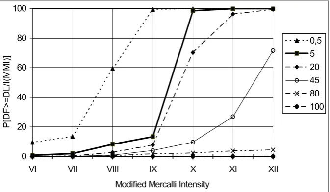
Figure 3. Fragility curves for medium-rise dual R/C systems regularly infilled with brick masonry walls, corresponding to ‘old’ buildings (Kappos et al. 2002b).

0 20 40 60 80 100

VI VII VIII IX X XI XII Modified Mercalli Intensity

P[DF>=DL/

Ι

(MMI)]

Figure 8. Comparison of the Grevena (top) and Düzce (bottom) microzonation study mean velocity spectra with the design spectra of the Greek and Turkish seismic codes and the mean spectrum of the records used for the derivation of fragility curves (Kappos et al. 2010).

0.00 0.50 1.00 1.50 2.00 2.50 3.00

0.00 0.50 1.00 1.50 2.00

Sv

(m

/sec

)

T (sec)

Fragility Curves Mean Spectrum

Grevena mean spectrum

Greek Code (Soil type Β)

0.00 0.50 1.00 1.50 2.00 2.50 3.00

0.00 0.50 1.00 1.50 2.00

Sv

(m

/sec

)

T (sec)