Interaction Effects on Common Measures of Sensitivity: Choice of Measure, Type I Error and Power
Stephen Rhodes1, Nelson Cowan1, Mario A. Parra2,3, and Robert H. Logie2
1Department of Psychological Sciences, University of Missouri
2Human Cognitive Neuroscience, Centre for Cognitive Ageing and Cognitive Epidemiology, Department of Psychology, University of Edinburgh
3Department of Psychology, Heriot-Watt University
Accepted for publication at Behavior Research Methods. June 26, 2018
Author Note
Part of this work was completed while the first author was at the University of Edinburgh and was supported by a PhD studentship from the Centre for Cognitive Ageing and Cognitive Epidemiology, part of the UK cross council Lifelong Health and Well-being Initiative (MR/L501530/1). S.R., N.C., and R.H.L are currently supported by the ESRC, Grant ES/N010728/1. Part of this work was presented at the 57th annual meeting of the Psychonomic Society in Boston. The code written to perform these simulations can be found here:
https://github.com/stephenrho/MeasuresAndErrors.
Abstract
Here we use simulation to assess previously unaddressed problems in the assessment of statistical interactions in detection and recognition tasks. The proportion of hits and false-alarms made by an observer on such tasks is affected by both their sensitivity and bias, and numerous measures have been developed to separate out these two factors. Each of these measures makes different assumptions regarding the underlying process and different predictions as to how false-alarm and hit rates should covary. Previous simulations have shown that choice of an inappropriate measure can lead to inflated type I error rates, or reduced power, for main effects, provided there are differences in response bias between the conditions being compared. Interaction effects pose a
particular problem in this context. We show that spurious interaction effects in analysis of variance can be produced, or true interactions missed, even in the absence of
variation in bias. Additional simulations show that variation in bias complicates patterns of type I error and power further. This under-appreciated fact has the
potential to greatly distort the assessment of interactions in detection and recognition experiments. We discuss steps researchers can take to mitigate their chances of making an error. (194 words)
Interaction Effects on Common Measures of Sensitivity: Choice of Measure, Type I Error and Power
In binary choice recognition and detection paradigms, observers are presented with a sequence of stimuli and are required to distinguish targets (for example, previously studied items) from non-targets (for example, new items). Performance on such tasks is captured by the proportion of target responses conditional on whether the probe was actually a target or not. Participants make a hit if they correctly identify a target, whereas they make afalse-alarm if they incorrectly characterize a non-target. The proportion of hits and false-alarms will not only be influenced by an observer’s ability to distinguish targets and non-targets (which is usually of primary interest to researchers), but also by their preference for one response option over another. Thus, researchers regularly adopt measures that aim to separate out the sensitivity of observers from their response bias. In order to do this, these commonly used measures make particular assumptions about the process underlying discrimination. If these assumptions are unfounded then researchers are at risk of concluding that two conditions differ in sensitivity when truly they differ in bias, or they may miss true differences between conditions (Rotello, Masson, & Verde, 2008; Schooler & Shiffrin, 2005).
Here we consider the assessment of interactions with commonly used single point estimates of sensitivity (d0, Pr, A0) and find that this presents a particular problem not
recognized before in the literature. Typically researchers interested in differences
(1978), but remain under-appreciated (Wagenmakers, Krypotos, Criss, & Iverson, 2012). Here we illustrate a previously unarticulated problem in interpreting interactions from binary choice detection or recognition experiments that build on these earlier observations.
The article is organized as follows; firstly, three commonly applied measures of sensitivity (d0,P
r,A0) and their assumptions are described. We then discuss previous
simulation studies that have looked at the issue of main effects with point estimates of sensitivity and outline the rationale for the present simulations examining interactions. Following this, we describe type I error and power simulations for the three oft-used measures under different generative assumptions. Extending the previous simulations on main effects, the present work demonstrates that the interpretation of interaction effects poses an even greater problem if the selected measure is inappropriate for the data at hand. Specifically, problems with interactions can arise even in the absence of variation in response bias. Finally, we discuss ways in which researchers may choose a measure which is appropriate for their data, provide an empirical example of how conclusions are liable to be affected if they don’t, and discuss approaches if no reasonable measure can be identified.
Commonly used Measures and their Assumptions
Two broad classes of model dominate the analysis of sensitivity in recognition or detection paradigms; namely, the signal detection and high-threshold accounts. We outline these models in turn along with their frequently used estimators of sensitivity.1 In addition, we discuss a measure outside of these models that is often used in an attempt to avoid making assumptions about the underlying discrimination process, and the arguments that have been made against this measure.
1The present analysis deals entirely with commonly used point measures of sensitivity derived from
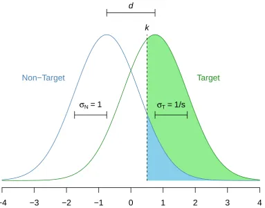
Signal Detection Theory. Accounts based on signal detection theory propose that items are evaluated on a continuous decision variable (Green & Swets, 1966; Tanner Jr & Swets, 1954). This evaluation is noisy (either due to the nature of the stimulus or the internal processing) but targets are expected to yield greater values on the decision variable than non-targets, producing two distributions (see Figure 1). The observer must establish a criterion, above which they respondtarget and below which they respondnon-target. Applications of signal detection theory tend to assume that the underlying evidence distributions are Gaussian as depicted in Figure 1. In this parameterization, the difference between the means of the two distributions is given by d. This parameter captures the sensitivity of the observer, which is their ability to
distinguish target and non-target items. As depicted in Figure 1, sensitivity is given in units of the standard deviation of the non-target distribution, which is fixed to 1 (without loss of generality). To account for the possibility that the two distributions have different variances, an additional parameter,s, controls the ratio of the non-target to target standard deviations. Consequently, the standard deviation of the target distribution is 1/s (as the non-target standard deviation is fixed to 1. See Figure 1). Here the criterion, k, is placed relative to the mid point between the means of the two distributions. According to this account, when a stimulus is presented, it elicits a value along the decision variable. As the observer does not know from which distribution this value has been sampled, they respond non-target if it is smaller thank and target if it is greater. Thus, negative k values indicate a liberal criterion (a bias toward responding
target), whereas positive values indicate a more conservative criterion (a bias toward respondingnon-target).
Assuming the distributions are normal, the probability an observer makes a hit is given by h= Φ[(d/2−k)/(1/s)], where Φ is the standard normal cumulative
−4 −3 −2 −1 0 1 2 3 4
Non−Target Target
d
k
σN=1 σT=1/s
Figure 1. Illustration of Gaussian signal detection theory. The parameterd determines the distance between the means of the non-target and target distributions, while σN
and σT give the standard deviations of these distributions. Finally, k is the criterion at
which the observer goes from responding non-target totarget. In this example, d= 1.5, k = 0.5, and s= 1 (equal variance). Hit rate is equal to the area of both the green and blue shaded areas. False-alarm rate is equal to the area of the blue area only.
order to derive a closed form estimator that translates pairs of false-alarm and hit rates into sensitivity, irrespective of response bias, it is necessary to restrict the s parameter (which controls the relative variance of the target and non-target distributions). Figure 1 depicts the case where s= 1 and, consequently, the distributions have equal variance. In this case a simple estimate of sensitivity can be determined by rearranging the above equations,d0 =z(h)−z(f), where z is the quantile function of the standard normal distribution (z(x) = Φ−1(x)). As the equation shows,d0 only serves as an estimate of d provided that the two distributions are standard normals with equal variances, otherwise sensitivity and bias will be confounded (Swets, 1986b).
[image:6.595.108.492.84.385.2]0.0 0.2 0.4 0.6 0.8 1.0
0.0
0.2
0.4
0.6
0.8
1.0
d'=
0
d'=
0.5
d'=
1
d'=
1.5
d'=
2.5
A
0.0 0.2 0.4 0.6 0.8 1.0
Pr=
0
Pr=
0.2
Pr=
0.4
Pr=
0.6
Pr=
0.8
B
0.0 0.2 0.4 0.6 0.8 1.0
A'=
0.5
A'=
0.65
A'=
0.8
A'=
0.9
A'=
0.95
C
false−alarm rate
hit r
ate
Figure 2. ROC curves predicted by (A) the Gaussian equal variance signal detection theory (σN =σT), (B) two high-threshold theory (PN =PT), and (C) the measure,A0.
between false-alarm rate and hit rate for a fixed level of sensitivity across all levels of bias. Figure 2A presents several ROC curves for different values of d0. This measure predicts symmetrical, curved ROCs that become more compressed to the top left of ROC space with incrementally increasing sensitivity. Relaxing the assumption of equal-variance (s6= 1) allows for asymmetrical ROC curves, that have often been
observed in the literature (Ratcliff, Sheu, & Gronlund, 1992; Swets, 1986a). The form of these ROC plots becomes particularly important when discussing evidence for
interactions, as will be shown later in detail.
High-Threshold Theory. Accounts based on threshold theory propose that, rather than items being evaluated on a continuum, observers enter one of a handful of discrete states (Luce, 1963; Snodgrass & Corwin, 1988). Consequently, the crucial quantities of interest are the probabilities of entering these states. According to this account, observers are said to either detect a certain state of affairs or be in a state of complete information loss and must guess. The most popular variant of threshold theory states that observers cannot detect an incorrect state of affairs (i.e. they cannot enter a target detect state when presented with a non-target and vice versa); that is, the thresholds are ‘high’ (see Snodgrass & Corwin, 1988). Figure 3 presents the
two-high threshold (THT) account of the detection process. The left tree indicates that, when a target is presented (as denoted by T), an observer has a specific probability, PT,
T
DT hit
!D
hit
miss
N
DN correct rejection
!D
false alarm
correct rejection
PT
1−PT
Br
1−Br
PN
1−PN
Br
1−Br
Figure 3. Illustration of the two-high threshold (THT) theory of detection. Diamonds refer to the nature of the item presented (T = target, N = non-target), circles refer to the internal state of the observer (DT = detect target, DN = detect non-target, !D = no detection), and rectangles refer to category of response made. Note that targets cannot lead to the detect non-target state and vice versa, making the model ‘high threshold’.
hit. On some proportion of trials (1−PT), however, the observer does not enter the
detect state, and must guess. The probability that the observer correctly guesses that the item is old is given by,Br. Zero bias towards responding target over non-target is
reflected in aBr of 0.5. The probability of correctly responding target, then, is the sum
of the branches in Figure 3 ending in a target response,h=PT + (1−PT)Br. On trials
where a non-target is presented (the right tree of Figure 3 beginning N), observers detect this at a rate of, PN. Therefore, a false-alarm can only occur if the detect
threshold is not passed and participants incorrectly guess. The probability of this occurring is given by, f = (1−PN)Br.
Constraints are needed to arrive at a point estimate of sensitivity from a pair of observed false-alarm and hit rates. Assuming that the probability of entering the target detection state is the same as the probability of entering the non-target detection state (PT =PN, referred to as Pr: Snodgrass & Corwin, 1988) results in a simple measure of
discriminability,Pr =h−f, which is commonly referred to as hit rate corrected for
guessing (or corrected recognition).
proportion correct, p(c), as an index of sensitivity. As noted by Macmillan and
Creelman (2005), the formula for proportion correct can be written as a linear function of hits minus false alarms, p(c) = 12(h−f) + 12. Thus, using proportion correct to summarize performance (sensitivity) in a recognition task implies a threshold decision model (see also Swets, 1986b), although this is rarely acknowledged. The two-high threshold model can also be expressed in a signal detection framework with rectangular underlying evidence distributions (see Rotello et al., 2008), however the
parameterization presented here more clearly outlines the rationale of this measure. The ROC curve predicted by the measure Pr is presented in Figure 2B. Unlike equal
variance signal detection, this account predicts linear functions within ROC space with an intercept of Pr and a slope of 1.
The measure A0. As noted by Pastore, Crawley, Berens, and Skelly (2003), the assumptions underlying measures of sensitivity, in particular signal detection theory, have caused some concern among researchers, who have gravitated towards the use of ostensibly assumption free, ‘non-parametric’ measures of sensitivity. The most popular measure in this vein isA0, which was developed by Pollack and Norman (1964) with the aim of estimating the area under the ROC curve. From the estimate of this area the researcher would obtain the expected proportion correct of an unbiased observer on a two-alternative forced choice task, irrespective of the underlying process (Green, 1964). This would achieve the goal of obtaining a truly assumption free measurement of an observers’ ability to distinguish targets from non-targets (Bamber, 1975; Green & Moses, 1966). With a single hit and false-alarm pair, however, it is only possible to get an average of the minimum and maximum areas implied.
high, A0 is consistent with a threshold model assuming (roughly) rectangular
distributions, as the ROCs are approximately linear. However, as performance lowers, the shape of the A0 ROC curve increasingly mimics that of a signal detection model assuming logistic evidence distributions (see Macmillan & Creelman, 1990, for a critique of bias measures associated with A0). No currently offered theory of recognition or detection makes the assumption that the underlying evidence distributions change with greater sensitivity, making this a problematic characteristic of A0. Further, while the initial aim behind the development of A0 was to obtain a compromise between the minimum and maximum areas implied by the single point, A0 fails to do this (see Smith, 1995; Zhang & Mueller, 2005). Despite these issues, A0 is still regularly used, so we include it in the present simulations. Grier (1971) and Aaronson and Watts (1987) provide the formulae for A0 for above and below chance performance, respectively:
A0 = 1
2 +
(h−f)(1 +h−f)
4h(1−f) , h≥f
A0 = 1
2 −
(f −h)(1 +f−h)
4f(1−h) , h < f.
Previous Simulations: Main Effects and Differences in Response Bias
Looking closely at Figure 2, one can see that for two conditions in which
participants have equal sensitivity, the different sensitivity metrics will be in agreement
provided that response bias is also equivalent. This is because, in this situation, the (f, h) pair from each condition occupies the same point in ROC space. As the effect of
changing bias is to move the (f, h) point along the ROC curve, differences between conditions in bias produce disagreements between different measures of sensitivity. For example, imagine two conditions generated by a signal detection process with the same sensitivity (d0) but where one condition has a neutral criterion and the other condition has a conservative response bias (i.e. k > 0). The more conservative condition is shifted along the same ROC curve as the neutral condition, but the effect of this is to produce a sensitivity difference when, say, Pr is calculated. This is an example of type I error,
different sensitivities (i.e. points on different ROC curves) appear to result in equal performance when an inappropriate measure is applied (i.e. a type II error). To our knowledge, two studies have looked at the ramifications of this via simulation.
Schooler and Shiffrin (2005) explored the efficacy of sensitivity measures when the available data are sparse due to small trial numbers per participant. Their simulated data were generated using a equal-variance signal detection model, in which two conditions either did or did not differ in terms of sensitivity. This allowed them to assess power and type I error rate, respectively. Provided the two conditions did not differ in terms of criterion placement or bias, the high threshold measure, Pr, performed
well, with type I error rates around the accepted value of 0.05. However, when
conditions differed in criterion placement, type I error rates for this measure were high (up to 34%) and, unsurprisingly, d0 performed better. When conditions truly differed in terms of sensitivity, power was greatly improved by using d0 relative to Pr, again
unsurprisingly as it matched the generative model.
Rotello et al. (2008) provided a more comprehensive set of simulations in which they generated data using either an underlying signal detection or two-high threshold structure. They assessed the type I error rates of repeated measures t-tests on multiple commonly used measures—including d0, A0 and proportion correct. They found that, with data simulated to have true differences in response bias between conditions, use of a measure not matching the assumptions of the generative model (e.g. applying Pr to
data simulated from a signal detection model) resulted in type I error rates typically in excess of 20%. Critically, the error rate associated with A0 was large regardless of the true underlying distributions. They also conducted power simulations for their
measures where there were true differences between hypothetical conditions in
The Present Simulations: Problems Interpreting Interactions, Even with
Equal Bias
The work of Schooler and Shiffrin (2005) and Rotello et al. (2008) clearly shows that, in the case of a comparison between two experimental conditions (or two groups), a misguided choice of sensitivity measure can result in errors provided there are
differences in response bias. The reason for this is clearly seen in the ROC plots
depicted in Figure 2; variation in bias between conditions results in two different points along the same ROC curve and, consequently, different measures of sensitivity give discrepant results.
One contribution of the present work is to point out that, for interactions between experimental conditions in ANOVA, it is possible for measures of sensitivity to produce discrepant results without any variation in response bias. The only condition that must be met for this disagreement to occur is that each experimental factor has a main effect on sensitivity.
To illustrate this, the simplest situation to consider is a 2 × 2 design; here we consider one between-subjects factor (e.g. age group) and one within-subjects
(experimental condition). Figure 4 depicts two situations where, in absence of variation in response bias,Pr and d0 would give opposing answers to the question of a group ×
condition interaction effect in a standard analysis of variance. The top row presents the case where for Pr there are two main effects but no interaction. However, whend0 is
calculated using the (f, h) pairs, a clear interaction effect emerges, where the effect of condition for group 1 is smaller than it is for group 2. The reason for this distortion can again be seen in the ROC plots of Figure 2; at increasingly high levels of sensitivity (d0) the curves implied by signal detection theory become more compressed and, thus, the equally spaced points in ROC space shown in Figure 2A imply increasingly large values of d0, resulting in an over-additive interaction. This analysis would imply that the effect of condition is larger for the higher performing group.
Group 1 Group 2 Cond 1 Cond 2
0.0 0.2 0.4 0.6 0.8 1.0
0.0
0.2
0.4
0.6
0.8
1.0
false−alarm rate
hit r
ate
1 2
1.0
1.5
2.0
2.5
3.0
3.5
d'
Condition
1 2
0.4
0.6
0.8
1.0
Pr
Condition
0.0 0.2 0.4 0.6 0.8 1.0
0.0
0.2
0.4
0.6
0.8
1.0
false−alarm rate
hit r
ate
1 2
1.0
1.5
2.0
2.5
3.0
3.5
d'
Condition
1 2
0.4
0.6
0.8
1.0
Pr
Condition
Figure 4. Plots showing that, when considering interactions, it is possible for the
commonly used two-high threshold and signal detection measures,Pr and d0, to disagree
without variation in bias. Top row: non-interaction with Pr but interaction usingd0.
Bottom row: interaction using Pr but main effects only with d0.
between conditions is smaller for the higher performing group. It is important to reiterate that this disagreement arises without any difference in response bias (all the points lie on the negative diagonal indicating neutral responding) and occurs when each experimental factor produces a main effect. No variation in bias and no main
experimental effects on sensitivity would result in four overlapping points in ROC space and, thus, no disagreement between the measures. Crucially, the data from this simple 2 ×2 design will not signal which is the correct measure to use. This decision must be based on empirical ROC data and other tests aimed at probing the generative process underlying the specific task in question (see the General Discussion).
great concern to researchers. The extent to which this has affected the literature on detection and recognition (especially that on group differences across different
experimental conditions) is difficult to gauge (although see Rotello, Heit, & Dubé, 2015, for examples where the choice of outcome measure may have greatly affected
conclusions). Simulation allows us to examine the extent to which these issues could conceivably cause problems in interpreting interactions for reasonable research designs. Consequently, in the present simulations we assess a wide range of parameter values, for both sensitivity and bias, across equal and unequal variance signal detection, and
two-high threshold generative models as well as assessing the influence of number of simulated subjects per group or trials per condition. There are potentially limitless combinations of these factors, so the code used to produce the present simulations is available at https://github.com/stephenrho/MeasuresAndErrorsfor researchers interested in assessing specific parameter settings. We report a subset of the simulations here which serve to illustrate, and elaborate on, the main points made so far. The results of all simulations are presented in Supplementary Material.
Structure of Simulations
Simulated data sets contained two groups of NS hypothetical subjects each
performing in two within-subjects conditions with the same number (NT) of target and
non-target trials per condition. Each set of trials was drawn from independent Binomial distributions, with the probability of a hit or false-alarm determined by the underlying model parameters (i.e. d and k, or Pr and Br) for a given subject in a given condition.
For both signal detection and two-high threshold simulations the underlying parameter values, p, that controlled sensitivity and bias were determined using the same linear equation:
pi,b,w =β0+β1xb +β2xw+β3xbxw+bi,
group) and W (within subjects, condition), respectively.2 The indicator variables, x
b
and xw, are set to −1 if the observation comes from the first level of the factor or to 1
for the second level. Consequently, positive values of our deflection parameters mean lower parameter values at level 1 relative to level 2. The value β3 is the multiplicative interaction between the two variables (xbxw); so as long asβ3 = 0 there is no interaction present in the simulated data set. The final component,bi, reflects random variation in
the parameter value due to theith simulated subject. This is assumed to be normally
distributed with a mean of zero and standard deviation, σS. Note that this only affects
the overall level of performance between hypothetical participants and there is no variability associated with the effect of the within subjects factor.
Both sensitivity (d or Pr) and bias (k or Br) parameters were determined using
this linear equation. These general parameters are referred to throughout this manuscript with superscripts denoting the model parameter to which they refer; for example, a main effect of group on sensitivity with a signal detection generative model would be indicated in the magnitude of β1(d), whereas an effect of condition on two-high threshold response bias is determined by β(Br)
2 . For the high threshold simulations, as the parameters are constrained to fall between 0 and 1 values outside this range were rounded up to 0 or down to 1. Each simulation proceeded as follows;
1. Parameter values for the generative model were derived for NS hypothetical
participants using the above equation with the present settings forβ0, β1, β2, and β3. Participant variability was sampled from a normal distribution with a mean of zero and a standard deviation,σS.
2. Predicted h and f rates were determined according to the generative model (see description of models above).
3. NT target and non-target trials were simulated for each condition for each subject
as samples from a Binomial distribution, with success probability determined by h 2In many applications of signal detection theory the symbolβ is used to refer to the likelihood ratio
for target trials and f for non-target trials.
4. d0, A0, and Pr were calculated with the simulated hit and false-alarm rates (see
formulae above).3
5. Steps 1-4 were repeated 1000 times per combination of parameter settings and ANOVAs were conducted on the resulting data sets to obtain the frequency of
p <0.05 for the group × condition interaction.
Here we focus on a subset of the type I and type II error simulations where there are no true condition or group differences in response bias. Full results of all the
simulations conducted are presented in Supplementary Material and the code to conduct them is available online: https://github.com/stephenrho/MeasuresAndErrors.
Type I Error Simulations
In these simulations, we were interested in assessing the type I error rates of the different measures in the absence of variation in response bias. To this end, we varied the overall sensitivity (controlled by the parameter β0 in the linear equation above) of our hypothetical observers as well as the main effects of group (β1) and condition (β2). To reduce the number of simulations, we fixed the size of the two main effects to be equal. In addition, we also assessed the effect of increasing the number of participants per group (NS) or trials per condition (NT) on error rate.
Two-High Threshold
For the simulations with the threshold model, the grand mean bias parameter (β(Br)
1 ) was set to 0.5 (neutral) and there were no main effects or participant variability in bias (that is, β(Br)
1 =β (Br)
2 =σ (Br)
S = 0). Of primary interest here was variability in
grand mean sensitivity (or probability of detection) and main effects of group and 3In calculatingd0, one encounters problems with undefinedzscores with proportions of 0 or 1. Prior
condition. Mean sensitivity (β(Pr)
0 ) was varied from 0.4 to 0.8 in steps of 0.1 and random participant variability in sensitivity was simulated by setting the standard deviation parameter, σ(Pr)
S , to 0.1. Our primary interest was in the influence of main
effects on sensitivity, so the main effect parameters for group (β(Pr)
1 ) and condition (β(Pr)
2 ) took the values 0, 0.025, 0.05, and 0.1, with the constraint that they were fixed to the same magnitude. Scaled in terms of the random intercept parameter mentioned above, these values represent no, small, medium, and large effects, respectively. These settings allowed us to cover a wide range of parameter values and hit/ false-alarm rates. The range of hit and false-alarm rates across simulations was comparable across the two-high threshold and signal detection simulations (presented next). For both, the most sensitive group and condition were expected to achieve almost perfect performance (h≈1,f ≈0; i.e. a ceiling effect), whereas the least sensitive group/ condition was close to chance (h≈.6, f ≈.4). Note that the main effects were also scaled in the same way relative to the random participant standard deviation parameter for both the THT and SDT simulations (0%, 25%, 50%, 100% for none, small, medium, and large,
respectively).
Finally, in separate simulation runs we varied the number of hypothetical subjects (NS) or the number of trials (NT) through 12, 24, 48. The results of increasing the
number of participants per group or trials per condition were practically identical, therefore we present the former here and the latter in the supplementary material (see Simulation 2).
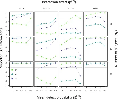
The results of this simulation with a threshold-generative model are presented in Figure 5. As can be seen in this figure, type I error rates remain under control until there are large main effects of group and condition. As shown in the rightmost panels, error rates for bothA0 and d0 depend on the overall level of discriminability (β(Pr)
0 ). The frequency of errors is more pronounced with d0 relative to A0 until the very highest grand mean sensitivity is reached, at which point the error rate for d0 drops to a similar level as Pr. As noted above, erroneously applying d0 to data conforming to the
Index
100
0.0 0.2 0.4 0.6 0.8 1.0
0
d' A' Pr
Index
100
0.025
Index
100
0.05
Index
100
0.1
12
Index
100
0.0 0.2 0.4 0.6 0.8 1.0
Index
100
Index
100
Index
100 24
Index
100
0.4 0.5 0.6 0.7 0.8 0.0
0.2 0.4 0.6 0.8 1.0
Index
100
0.4 0.5 0.6 0.7 0.8
Index
100
0.4 0.5 0.6 0.7 0.8
Index
100
0.4 0.5 0.6 0.7 0.8
48
Mean detection probability (β0(Pr)) Detection main effects (β1(Pr)= β2(Pr))
Number of subjects (
NS
)
Propor
tion Sig. Inter
actions
Figure 5. Type I error rates for d0, A0, and Pr with an underlying two-high threshold
(THT) model. This simulation varied overall detection probability (xaxis), magnitude of main effects on detection (left to right), and number of simulated participants (top to bottom).
differences between conditions are larger in groups that are more sensitive overall (an
over-additive interaction effect). As overall performance improves (moving along the x-axis), this distorting effect becomes even larger, rising to an error rate in excess of
80% with groups of 48 hypothetical subjects. The ceiling effect encountered at high underlying levels of sensitivity (yeilding hit rates around 1 and false-alarm rates around 0 in the highest performing group) reduces thisover-additive tendency, seen as a drop of error rate at the highest mean sensitivity in Figure 5. The effect of ceiling
discriminability on type I error rate is also seen when the correct measure,Pr, is applied
pattern of means (Rotello et al., 2015).
In further simulations, we introduced individual differences in bias (Br) and varied
the overall grand mean bias, which did not affect the pattern of errors greatly (see Simulation 4 in supplement). Introducing main effects of both group and condition on response bias, along with the main effects on sensitivity, had a big effect on errors, however. This was especially true for d0, whose errors were magnified by a conservative overall bias (i.e. Br <0.5) and large main effects on this parameter. As a logical
extension of the simulations reported by Rotello et al. (2008) and Schooler and Shiffrin (2005), we also assessed the effect of manipulating bias between groups and conditions in the absence of true main effects on sensitivity. d0 was the only measure to exhibit inflated type I errors in this simulation (around 20%) when the bias effects were large. Interested readers can find the full results of these simulations in the supplementary material accompanying this article.
Signal Detection
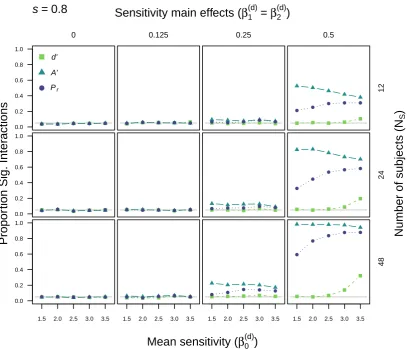
According to the formulation of the signal detection model described above (see Figure 1), a criterion of zero represents a neutral bias. Therefore, for these simulations the grand mean criterion (β0(k)) was fixed to 0 and there were no main or participant effects on criterion placement (β1(k) =β2(k) =σS(k)= 0). Overall sensitivity was varied by having the grand mean parameter (β0(d)) take several values (1.5, 2, 2.5, 3, 3.5).
Similarly, the magnitude of the main effects of group (β1(d)) and condition (β2(d)) on sensitivity were also varied (0, 0.125, 0.25, 0.5) with the two fixed to be the same value. The random participant effect had a standard deviation (σS(d)) of 0.5. These settings allowed us to cover a wide variety of parameter values and hit/ false-alarm rates. As in the previous simulations with a threshold generative model, combinations of these parameter settings were assessed with varying numbers of hypothetical subjects or (in a separate run) varying numbers of trials. Once again the results of these two sets of simulations were remarkably similar (see Simulation 2 in the supplementary material).
Index
100
0.0 0.2 0.4 0.6 0.8 1.0
0
d' A' Pr
Index
100
0.125
Index
100
0.25
Index
100
0.5
12
Index
100
0.0 0.2 0.4 0.6 0.8 1.0
Index
100
Index
100
Index
100 24
Index
100
1.5 2.0 2.5 3.0 3.5 0.0
0.2 0.4 0.6 0.8 1.0
Index
100
1.5 2.0 2.5 3.0 3.5
Index
100
1.5 2.0 2.5 3.0 3.5
Index
100
1.5 2.0 2.5 3.0 3.5
48
Mean sensitivity (β0(d)) Sensitivity main effects (β1(d)= β2(d))
Number of subjects (
NS
)
Propor
tion Sig. Inter
actions
Figure 6. Type I error rates for d0, A0, and Pr with an underlying Gaussian
equal-variance signal detection theory (EV-SDT) model. This simulation varied overall detection sensitivity (xaxis), magnitude of main effects on sensitivity (left to right), and number of simulated participants (top to bottom).
underlying equal variance signal detection model. A couple of noteworthy patterns standout; firstly, error rates for all measures are at, or around, the conventionally accepted rate of 0.05 when there are no main effects or the true main effects of group (the between-subjects factor) and condition (the within-subjects factor) on sensitivity are small. When there are medium-to-large main effects, the error rates for A0 and Pr
depart from accepted levels, and increasing the number of participants per group
exacerbates this (Figure 6 right-hand panels). Of the measures, A0 clearly is more likely to erroneously give evidence for an interaction effect where none exists.
becomes increasingly problematic as the underlying sensitivity increases, whereas for A0 errors become somewhat less pronounced as mean sensitivity increases. For both of these measures, however, when there are large main effects, the type I error rate is unacceptable (around 0.7 for Pr and 0.8 for A0 with 24 participants per group). d0 also
exhibits exacerbated error rates for the interaction test when underlying sensitivity is high and there are large main effects, despite the fact that this measure is consistent with the generating model. This is clearly due to a ceiling effect, which restricts performance of the highest performing group, producing an under-additive interaction where the effect of condition appears smaller in the better performing group. This begins to appear in the simulations where grand mean sensitivity (β0(d)) is 3 and the main effects are large (0.5). In this case the expected hit and false-alarm rates of the highest performing group are 0.98 and 0.02, respectively.
We also conducted several simulations in which bias was allowed to vary, the results of which are presented in the supplement. To summarize, allowing for individual differences and overall shifts in criterion placement (i.e. non-neutral) had a small effect on error rates. Mainly, type I error rates for all three measures were less pronounced as the observers departed from neutral overall responding, either towards a liberal or conservative criterion placement. Introducing main effects of both variables had a pronounced effect on error rates (see Simulation 6 in supplement). As the size of these main effects increases, type I error rates rise for both Pr and A0, particularly when the
overall criterion placement is neutral. We discuss reasons for this pattern of results in the supplement. This tendency for main effects on criterion placement to inflate type I errors for interactions was also present when main effects on sensitivity were removed (see Simulation 7). Thus, in line with previous findings concerning type I error for main effects (Rotello et al., 2008; Schooler & Shiffrin, 2005), it is possible to generate
spurious interactions purely from differences in response bias.
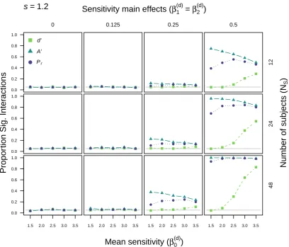
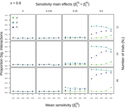
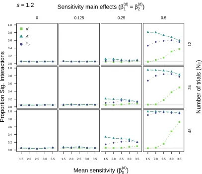
also looked at situations where targets produced a more variable distribution over the decision variable than non-targets (s= 0.8) and vice versa (s = 1.2). For each
simulation the same general patterns of type I error rates (and power, see below) were visible as in the equal variance case, although they were slightly less pronounced for s= 0.8 and slightly more pronounced fors= 1.2. Interested readers can find the full results of these simulations in the online supplementary material.
Summary of type I error simulations
The simulations reported above (and those in the supplement) confirm the
argument made on the basis of Figure 4 and show that choosing a measure of sensitivity that mismatches the model underlying the decision process can lead to spurious
evidence for interaction effects in detection or recognition experiments. Crucially, this happens without systematic variation in response bias when the factors in the
experimental design produce main effects. In follow up simulations, we fixed the number of participants per group and trials per condition to 24 and orthogonality varied the magnitude of group and condition main effects. This confirmed that as long as one effect is large and the other is at least medium in size, inflated type I error rates occur (see Simulation 3 in the supplement).
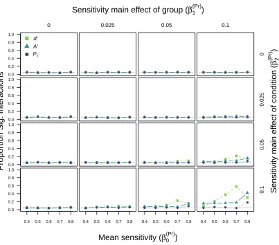
Power Simulations
Another implication of Figure 4 is that there are likely to be occasions where actual interaction effects on the correct scale of measurement are missed. Specifically, it seems that over-additive interactions with a signal detection underlying model may be missed by choosingPr, whereas an under-additive interaction on two-high threshold’s
detection parameter may be missed with d0. The next set of simulations addressed this. As described above in the Structure of Simulations section, the indicator variables xb and xw were set to −1 if the observation came from the first level of the factor or to
1 for the second level. Using positive values of our β1 and β2 coefficients is then useful for simulating interaction effects in the current context. A negative coefficient for the interaction (β3) produces an under-additive interaction effect, where the effect of condition is less pronounced for the better performing group (or, equivalently, group differences are less pronounced in the easier condition). A positive coefficient, on the other hand, produces an over-additive interaction where there is a greater effect of condition in the higher performing group (or a greater group difference in the easier condition). We used this to assess the power (1− type II error) of the three measures under different generative models. There was no variation in response bias between groups, conditions, or individuals. We examined power under varying numbers of participants per group (presented here) and trials per condition (presented in the supplementary material, Simulation 9).
Two-High Threshold
This set of simulations used the same general parameter settings as the earlier type I error simulations, but this time introduced interaction effects that were either under- or over-additive. As mentioned above, negative values of β(Pr)
3 produce
under-additive interactions, whereas positive values produce over-additive interactions. This parameter was varied through, −0.05, −0.025, 0.025, 0.05.
effects on sensitivity were large (β(Pr)
1 =β (Pr)
2 = 0.1). It is in this condition where the differences between measures were most pronounced, however we summarize the other results here. At a small main effect size (β(Pr)
1 =β (Pr)
2 = 0.025) power for the interaction effect was more-or-less identical for all three measures. Power began to diverge between measures for the medium main effect size (0.05), with d0 slightly under-powered for under-additive interactions and somewhat overpowered (relative to the correct measure, Pr) for over-additive interactions, as we would predict from Figure 4. Figures depicting
these findings are presented in the supplement under Simulation 8.
Index
100
0.0 0.2 0.4 0.6 0.8 1.0
−0.05
Index
100
−0.025
Index
100
0.025
Index
100
0.05
12
Index
100
0.0 0.2 0.4 0.6 0.8 1.0
Index
100
Index
100
Index
100 24
Index
100
0.4 0.5 0.6 0.7 0.8 0.0
0.2 0.4 0.6 0.8 1.0
d' A' Pr
Index
100
0.4 0.5 0.6 0.7 0.8
Index
100
0.4 0.5 0.6 0.7 0.8
Index
100
0.4 0.5 0.6 0.7 0.8
48
Mean detect probability (β0(Pr)) Interaction effect (β3(Pr))
Number of subjects (
NS
)
Propor
tion Sig. Inter
actions
Figure 7. Power for d0, A0, and Pr with an underlying two-high threshold (THT) model.
This simulation varied overall probability of detection (x axis), the magnitude and direction of interaction (left to right) and the number of participants per group (top to bottom). Note: this figure depicts the case where main effects on detection equal 0.1.
[image:24.595.86.500.280.631.2]right ones it is clear to see that, relative to the correct measure Pr,A0 is overpowered4
for under-additive interactions (left) and tends to miss over-additive interactions
(right). This pattern is reversed for d0, which tends to miss under-additive interactions, as indicated by its low power. Figure 4 provides the explanation for this, in that
conversion ofPr onto d0 scale produces an exaggeration of differences at higher levels of
sensitivity; therefore, when the ‘true’ interaction is under-additive the two cancel each other out to a large extent. Finally, Pr appears to miss over-additive interactions at
very high levels of performance due to a ceiling effect for the most sensitive group, which limits the visibility of the over-additive interaction (see rightmost panels).
Once again, in additional simulations, presented in full in the supplement, we also assessed the effect of manipulating bias on power. Introducing participant variability and different overall levels of bias did not affect estimates greatly. Adding large main effects on response bias complicated things further and was sufficient to cause
distortions in power even without group or condition effects on sensitivity.
Signal Detection
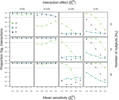
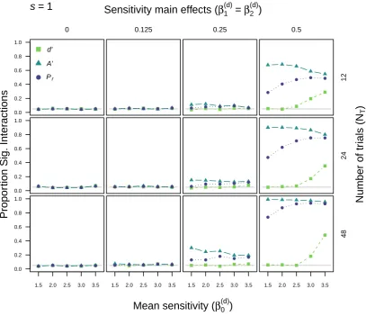
For the signal detection simulations, we used the same parameter values as the initial type I error simulations with the additional interaction effect on sensitivity (β3(d)), which could either be under-additive (−0.25,−0.125) or over-additive (0.125, 0.25).
At a small main effect on sensitivity (β1(d)=β2(d) = 0.125) there is not much separating the measures in terms of power. With 24 participants in each group and a larger interaction effect (−0.25 or 0.25), power is always well above 80%. The measures diverge with two slightly bigger main effects (0.25), with A0 and Pr producing more
misses, relative to d0, for under-additive interactions but exhibiting artificially inflated power for over-additive interactions. The clearest divergence is shown in Figure 8 which depicts the results of simulations with two large main effects (0.5) on sensitivity. The results not depicted here can be found in the supplementary material.
As can be seen in Figure 8, when the true generative model consists of a small 4It is worth noting that being ‘overpowered’ is not a good thing in this case, as it arises from an
Index
100
0.0 0.2 0.4 0.6 0.8 1.0
−0.25
d' A' Pr
Index
100
−0.125
Index
100
0.125
Index
100
0.25
12
Index
100
0.0 0.2 0.4 0.6 0.8 1.0
Index
100
Index
100
Index
100 24
Index
100
1.5 2.0 2.5 3.0 3.5 0.0
0.2 0.4 0.6 0.8 1.0
Index
100
1.5 2.0 2.5 3.0 3.5
Index
100
1.5 2.0 2.5 3.0 3.5
Index
100
1.5 2.0 2.5 3.0 3.5
48
Mean sensitivity (β0(d)) Interaction effect (β3(d))
Number of subjects (
NS
)
Propor
tion Sig. Inter
actions
Figure 8. Power ford0, A0, and Pr with an underlying Gaussian equal variance signal
detection theory (SDT) model. This simulation varied overall sensitivity (x axis), the magnitude and direction of interaction (left to right) and the number of participants per group (top to bottom). Note: this figure depicts the case where main effects on
sensitivity equal 0.5.
under-additive interaction and a small sample size per groupA0 and Pr produce higher
estimates of power than the correct measure,d0, due to their tendency to distort data conforming to a signal detection model (see Figure 4). Their theoretical ROCs do not imply the same compression towards the top-left of ROC space thatd0 does and, consequently, they make differences at higher levels of performance appear less
pronounced. This is inverted for over-additive interactions, for the exact same reason, and d0 has consistently greater power, except for cases where ceiling level sensitivity quashes the interaction effect (as can be seen progressing along the x-axis). A0 performs particularly badly for a large over-additive interaction (see right most panels of
[image:26.595.85.503.83.434.2]Additional power simulations, in which overall criterion placement was varied, showed that for over-additive interactions the power of the correct measure, d0 dropped as criterion deviated from neutral, whereas power with Pr was inflated. Adding main
effects on criterion placement complicated things a great deal (see the supplement for in depth discussion) and was sufficient to distort estimates of power even in the absence of main effects on the sensitivity parameter.
Summary of power simulations
The power simulations reveal a complex set of results wherein evidence for interactions is either suppressed or erroneously magnified, depending on the nature of the true interaction effect (either under- or over-additive) and the generative model. Analyses of interactions conforming to a two-high threshold discrimination process with the measure d0 tend to miss under-additive effects, where group differences are
suppressed in higher performing conditions. Applying A0 to this data, however, one would be liable to miss over-additive interactions where group differences are more pronounced at higher performance levels. With data conforming to a signal detection theory account, applying A0 orPr will lead to an increased likelihood of missing a true
over-additive interaction effect. This happens because of the different scaling implied by the different measures and does not rely on variation in bias, although adding this variation complicates matters further (see Supplement).
General Discussion
Binary choice recognition or detection performance summarized in terms of hit and false-alarm rates confounds the observer’s ability to perform the discrimination with their inherent bias towards one of the response options. In order to separate the contribution of these two factors, a model of the underlying decision process is needed. Commonly used measures, d0 and Pr, come from two broad classes—those that assume
a continuous decision variable, with observers comparing sampled values to a criterion, and those assuming a handful of discrete states—and are particularly restricted
not specify the basic process underlying the discrimination but, that being said, does
imply specific evidence distributions and ROC curves (Macmillan & Creelman, 1996). Previous work has established that, if a measure is applied that does not conform to the underlying structure of the data, two conditions may appear to differ in
performance (i.e. sensitivity) where no true difference exists, provided that they differ in response bias (Rotello et al., 2008; Schooler & Shiffrin, 2005). In the present case we were interested in conclusions regarding interactions between variables assessed via analysis of variance. The simulations presented here (and in the online supplementary material) have shown that erroneous conclusions can arise regarding interactions between variables in the absence of any difference in response bias. In the examples used here, provided both group and condition resulted in moderate to large main effects themselves, the probability of erroneously encountering a significant interaction effect is quite large when an inappropriate measure is applied. Further, genuine interaction effects are likely to be missed; with a specific tendency for d0 to miss under-additive interactions and for Pr to miss over-additive interactions (see Figure 4). These
simulations show how various factors, such as the overall sensitivity of observers, differences between groups and conditions, and variation in response bias, combine to influence error rates and power.
The problem of understanding the theoretical importance of interactions, such as these, were well outlined by Loftus (1978) who distinguished ‘interpretable’ and
‘uninterpretable’ interactions. The present simulations underline the problems
Recommendations
As we have described so far, assessing the evidence for interaction effects is more difficult than it may first appear. In the field of recognition and detection, however, there are ways that researchers may gain greater confidence in the veracity of their interaction effects. Table 1 summarizes a number of steps researchers might take to avoid the problems highlighted in the simulations presented here. The remainder of the article covers these recommendations in more detail.
Choosing an appropriate measure. The importance of selecting a measure consistent with the structure of the data has been highlighted several times before (Macmillan & Creelman, 2005; Rotello et al., 2008; Swets, 1986a). But, as recently noted by Rotello et al. (2015), there is a tendency for outcome measures to be chosen on the basis of what is typically used in the field, without consideration of whether the measure gives an accurate representation of the underlying process. As outlined in the
Introduction, the source of the discrepancy between measures is in their different
predictions as to how false-alarm and hit rates should relate over varying response bias; that is, their predicted ROC curves (see Figure 2). The form of these ROC curves need not remain a mystery, however. Researchers should search the existing literature for empirical ROC curves constructed for tasks similar to their own (Swets, 1986a).
This is not without its pitfalls, and researchers should be wary of the controversy surrounding ROC curves derived from ratings procedures, in which, instead of a yes/no decision, participants rate their decision on a scale fromsure target to sure non-target. With such a ratings procedure, it is not necessarily the case that a threshold model predicts linear ROCs, as a change in the mapping of detection states onto ratings can introduce curvature (see Bröder, Kellen, Schütz, & Rohrmeier, 2013; Malmberg, 2002). Thus, it has been argued that analysts should focus on the form of binary choice ROC curves, derived from the manipulation of base rates (i.e. expectation of the frequency of target trials), or payoffs (i.e. offering more or less reward for correct target responses) (see Bröder & Schütz, 2009).
disciplines or tasks, and several such reviews already exist (Dube & Rotello, 2012; Macmillan & Creelman, 2005; Swets, 1986a; Wixted, 2007; Yonelinas & Parks, 2007). However, we are able to give an example of choosing an appropriate measure from our own field of interest (and what happens when an inappropriate measure is applied). Isella, Molteni, Mapelli, and Ferrarese (2015) recently used a change detection paradigm to assess younger and older adults’ short-term recognition memory for simple objects made up of color and shape. They were interested in the extent to which healthy aging affected the ability to detect changes to color-shape pairing beyond any age effect observed for detecting changes to individual features. In this case, a group by condition interaction may suggest that older adults have a specific deficit in short-term memory binding.
To address this question, the authors applied A0, claiming that it was “the most classical and appropriate parameter for a change detection task” (p. 38); however, it is not clear how this conclusion was reached. Nevertheless, Isella et al. (2015) found a significant group by condition interaction with this measure. In the online supplement to their paper, however, they report an additional analysis of proportion correct in which the crucial interaction is not significant. It is important to note that Isella et al. (2015) employed an adjustment for multiple comparisons which led them to dismiss the interaction contrast between the lowest performing individual feature condition (shape only) and the condition requiring color-shape binding (p=.021) as non-significant. As we argue below, this was likely a good move, however, given that this group by
condition interaction was the component of primary interest in this study, we can equally envisage a situation where the correction was not applied and the significant interaction interpreted in a different manner. Thus, we are using this as a case where different conclusions could have been reached based on the choice of measure, not as a specific critique of the conclusions of Isella et al. (2015).
achieved by varying the proportion of target and non-target trials and informing
participants of this, yield linear ROC curves when categorically distinct stimuli are used (e.g. Rouder et al., 2008). Thus, it can be argued that proportion correct, which can be justified as an index of sensitivity according to a high-threshold model (see above), is a more appropriate measure for the data of Isella et al. (2015). Indeed, other studies on the same topic have applied the two-high threshold measure, Pr, and have provided
evidence against the group by condition interaction (see Rhodes, Parra, & Logie, 2016; Rhodes, Parra, Cowan, & Logie, 2017).5
Nevertheless, it is often difficult to find truly diagnostic ROC curves (see, for example, the debate in the recognition memory literature; Bröder & Schütz, 2009; Dube & Rotello, 2012). Researchers should therefore consider additional sources of
information to help them decide between measures. For instance, recent interest has shifted from comparing models on the basis of ROC data towards tests of critical predictions made by models of the discrimination process. An example of this is the prediction of conditional independence made by the two-high threshold model (see Chen, Starns, & Rotello, 2015; Province & Rouder, 2012, for recent tests of this
prediction). This is the expectation that given a certain internal state (e.g. detection of a previously studied stimulus) has been reached, responses (e.g. confidence ratings) should be invariant and not depend on experimental manipulation. Assessments of the predictions of signal detection and high-threshold accounts regarding distributions of reaction times are also informative in arriving on an appropriate measure for a given situation (see Donkin, Nosofsky, Gold, & Shiffrin, 2013; Dube, Starns, Rotello, &
5When considering change detection it is worth noting that there are a range of other measures that
Ratcliff, 2012; Province & Rouder, 2012).
In the process of searching for a measure it is highly likely that a measure outside of the set considered here will be appropriate for the paradigm under consideration. It is then useful for applied researchers to be aware of other models and measures that they may add to their toolkit. For example, even if the data conform to a Gaussian signal detection model, it may be that the evidence distributions have different
variance, making the use of d0 inappropriate (Swets, 1986a). Previous estimates of the ratio of non-target to target standard deviations (s) can be used to correct d0 to be more appropriate to the underlying structure of the data. In recognition memory
paradigms, for example, ROC estimates ofs tend to be smaller than 1 at approximately 0.8 (see Ratcliff et al., 1992; Wixted, 2007). It is possible, given a previous estimate of s, to obtain an appropriate estimate of sensitivity according to a signal detection
account. One such measure isda (Simpson & Fitter, 1973), which gives the separation
of the target and non-target distributions in terms of the root mean square of the two standard deviations. The formula for calculating this measure can be found on page 400 of Rotello et al. (2008).
a detailed discussion of this important point). Knowledge of these alternative measures and models, often ignored in applied research, will better place researchers to avoid erroneous conclusions regarding interactions.
Avoid ceiling level performance. Avoiding perfect, or near perfect,
performance is usually a concern for researchers. The present simulations reinforce this concern by clearly showing that high levels of performance can cause issues even when an appropriate measure is chosen. The simulations with variable response bias also reveal a problem wheneither h orf are at ceiling (or floor), as this results in the other estimated rate coming to dominate inference, which in turn can drive erroneous
conclusions even when the correct measure is applied. Thus, while overall performance (e.g. proportion correct) may not be at ceiling, individual rates of 0 and 1 can still cause problems. The supplementary material contains further discussion of this point.
Consider the scale of measures. When there is no variation in response bias, the primary source of disagreement between measures in an analysis of variance stems from the way in which they are scaled. Equal increments along the negative diagonal imply increasingly smaller differences in d0 (Figure 2A), whereas the way in which our two-high threshold simulations were set up reflects the general assumptions implied in analyzing estimates of Pr with ANOVA. That is, that Pr is on an interval scale so that
mean differences are equally as meaningful at moderate and high levels of sensitivity. It seems unlikely that researchers would ascribe as great a meaning to a difference in Pr of
0.55 vs 0.6 as they would to the difference between 0.9 and 0.95. These scaling issues are often raised when discussing the analysis of categorical data, so analyses assuming a high threshold process may benefit from insights from this area.
As noted in the Introduction, proportion correct can be justified as a measure of sensitivity given its linear relation to Pr. To reflect the assumption that differences at
higher levels of accuracy are more meaningful than differences at lower levels,
researchers may analyze a transformation of proportion correct. Logit models offer one such method of analysis, which is preferable to the analysis of aggregated and
estimate the log odds of a correct response (across both target and non-target trials) using the raw binary (correct and incorrect) responses. This analysis would still imply linear ROCs but would produce a similar scaling of effects to that produced with the signal detection theory measure, d0 (the z, or probit, transformation used in calculating d0 is very similar to the log odds, or logit, transformation). Consequently, one avoids the problem of treating Pr as if it were interval in scale (as is implied in the use of
ANOVA), and scales effects similarly to a signal detection theory analysis.
To show this, we fit a mixed-effects logit model to each simulated data set from the first series of simulations that used an equal variance signal detection generative model. P-values for group by condition interactions were obtained using the lme4 package in R
(Bates, Maechler, Bolker, & Walker, 2014; R Core Team, 2015). As expected, relative to ANOVA on Pr, the logit model fared much better with type I error rates, on average,
approximately 13% lower. Overall, there was no clear difference between the logit model and the correct measure d0 (on average, type I error rates differed by 0.5%). Thus, changing the way in which one thinks about the scale of effects on Pr, which seems
reasonable given that this measure is bounded by 0 and 1, reduces the disagreement between models in the absence of variation in response bias. Disagreement still arises when bias is varied between groups and conditions, as exemplified by the simulations in which there were no main effects on sensitivity (see Simulations 7 and 12 in
supplementary material) (see also Rotello et al., 2008; Schooler & Shiffrin, 2005).
Present a range of measures. It is likely that researchers will be faced with a situation where there is no good reason to pick a particular measure over others
available. For example, a researcher may design a task for which no good ROC evidence exists and they are unable, due to lack of time or resources, to probe this themselves. In this case what can they do? Many of the options open to researchers in this
circumstance have already been outlined by Wagenmakers et al. (2012, pp. 157). Perhaps the simplest is that investigators may choose to report a range of different measures, such as d0,Pr, logit(p), as well as signal detection measures that do not
survives (or whether additivity remains). If an interaction effect appears with multiple measures, one can gain confidence that their conclusion is not dependent on a single scale of measurement (although doubtlessly it will vary in magnitude, in which case a range of effect sizes may be given).
Alternative ways of assessing of sensitivity. The frequent use of the
measureA0 suggests that—possibly due to an (implicit or explicit) understanding of the issues above—researchers are not comfortable with the underlying assumptions made by other measures of sensitivity, and desire an assessment of performance that is not tied to a particular conception of the discrimination process. However, as outlined in the
Introduction,A0 does not live up to its ‘non-parametric’ name (Macmillan & Creelman, 1996) and there have been repeated calls for use of the measure to be reconsidered or abandoned (Pastore et al., 2003; Rotello et al., 2008). Our simulations add to the long list of reasons to avoid this measure. In type I error simulations, A0 performed
particularly badly when data conformed to the expectation of a signal detection model and did not fare well at detecting over-additive interactions for both generative models considered here. However, the desire to have a measure of performance which is tied to as few assumptions as possible remains.
Alternatively, if the target/ non-target decision is not integral to the study design, researchers may consider a two-alternative forced choice (2AFC) task in which observers are presented with two items (one a target and one a non-target) and must select one of them as the target. In many applications it may be safely assumed that bias plays little role in responding and does not vary greatly between conditions or groups. Thus the 2AFC can reduce concerns regarding the separability of sensitivity and bias, but measurement decisions still need to be made (see Macmillan & Creelman, 2005, Chapter 7 for detailed discussion).
A summary of recommendations, along with their strengths and drawbacks, can be found in Table 1.
Concluding Remarks
References
Aaronson, D., & Watts, B. (1987). Extensions of Grier’s computational formulas for A’ and B” to below-chance performance. Psychological Bulletin, 102(3), 439–442. Bamber, D. (1975). The area above the ordinal dominance graph and the area below
the receiver operating characteristic graph. Journal of Mathematical Psychology,
12(4), 387–415.
Bates, D., Maechler, M., Bolker, B., & Walker, S. (2014). lme4: Linear mixed-effects models using Eigen and S4 [Computer software manual]. Retrieved from
http://CRAN.R-project.org/package=lme4 (R package version 1.1-7)
Bröder, A., Kellen, D., Schütz, J., & Rohrmeier, C. (2013). Validating a
two-high-threshold measurement model for confidence rating data in recognition.
Memory, 21(8), 916–944.
Bröder, A., & Schütz, J. (2009). Recognition ROCs are curvilinear—or are they? on premature arguments against the two-high-threshold model of recognition. ,
35(3), 587–606.
Brown, S. D., & Heathcote, A. (2008). The simplest complete model of choice response time: Linear ballistic accumulation. Cognitive Psychology, 57(3), 153–178.
Chen, T., Starns, J. J., & Rotello, C. M. (2015). A violation of the conditional
independence assumption in the two-high-threshold model of recognition memory.
Journal of Experimental Psychology: Learning, Memory, and Cognition, 41(4), 1215–1222.
Cowan, N., Blume, C. L., & Saults, J. S. (2013). Attention to attributes and objects in working memory. Journal of Experimental Psychology: Learning, Memory, and Cognition, 39(3), 731–747.
Dixon, P. (2008). Models of accuracy in repeated-measures designs. Journal of Memory and Language, 59(4), 447–456.