City, University of London Institutional Repository
Citation
:
Slabaugh, G. G., Gundry, M., Knapp, K., Asad, M. and Al Arif, S. M. M. R.
(2017). Patch-based Corner Detection for Cervical Vertebrae in X-ray Images. Signal
Processing: Image Communication, doi: 10.1016/j.image.2017.04.002
This is the accepted version of the paper.
This version of the publication may differ from the final published
version.
Permanent repository link:
http://openaccess.city.ac.uk/17209/
Link to published version
:
http://dx.doi.org/10.1016/j.image.2017.04.002
Copyright and reuse:
City Research Online aims to make research
outputs of City, University of London available to a wider audience.
Copyright and Moral Rights remain with the author(s) and/or copyright
holders. URLs from City Research Online may be freely distributed and
linked to.
City Research Online: http://openaccess.city.ac.uk/ [email protected]
PATCH-BASED CORNER DETECTION FOR
CERVICAL VERTEBRAE IN X-RAY IMAGES
S M Masudur Rahman Al Arif1, Muhammad Asad1, Michael Gundry2, Karen Knapp2
and Greg Slabaugh1
1Department of Computer Science, City, University of London
2University of Exeter Medical School
Abstract
Corners hold vital information about size, shape and morphology of a vertebra in an x-ray image, and recent literature [1, 2] has shown promising performance for detecting vertebral corners using a Hough forest-based architecture. To provide spatial context, this method generates a set of 12 patches around a vertebra and uses a machine learning approach to predict corners of a vertebral body through a voting process. In this paper, we extend this framework in terms of patch generation and prediction methods. During patch generation, the square region of interest has been replaced with data-driven rectangular and trapezoidal region of interest which better aligns the patches to the vertebral body geometry, resulting in more discriminative feature vectors. The corner estimation or the prediction stage has been improved by utilising more efficient voting process using a single kernel density estimation. In addition, advanced and more complex feature vectors are introduced. We also present a thorough evaluation of the framework with different patch generation methods, forest training mechanisms and prediction methods. In order to compare the performance of this framework with a more general method, a novel multi-scale Harris corner detector-based approach is introduced that incorporates a spatial prior through a naive Bayes method. All these methods have been tested on a dataset of 90 X-ray images and achieved an average corner localization error of 2.01 mm, representing a 33% improvement in localisation accuracy compared to the previous state-of-the-art method [2].1
Keywords: Cervical, X-ray, Vertebra, Corner detection, Hough forest, Machine learning, Harris corner
1. Introduction
Evaluation of a cervical spine injury in an X-ray image is a major radiological challenge for an emer-gency physician. Studies show that 44% of cervical spine injuries are misdiagnosed due to misinterpreta-tion [3] and up to 67% of patients with missed cervical fractures suffered neurological deterioramisinterpreta-tion [4]. In order to decrease the risk of misinterpretation, automated image analysis algorithms can assist the emergency physicians. But applying these techniques on X-ray images has its own challenges due to low contrast, noise, and inter-patient variability.
In the past decade, researchers have tried to solve different problems on several radiographic mediums and body regions. A Hough transform-based method has been demonstrated in order to locate the ver-tebrae position, orientation and size in cervical X-ray images [5]. Another random forest based global spine localization algorithm has been presented in [6]. In [7], a 3D atlas-based method was proposed to locate the vertebra column in Computer Tomography (CT) scans. Dong et al. [8] utilized a probabilistic graphical model to measure the size and orientation and to identify cervical vertebrae on X-ray images. A layered framework of regression forest and hidden Markov model is proposed in [9] to localize vertebra centers in CT scans. Segmentation of the cervical vertebrae is addressed in [10–12]. The most popular techniques for segmentation are active shape models (ASM) and active appearance models (AAM) [11– 16]. However, both ASM and AAM require a good initialization of the mean shape near the optimal
segmentation. Corners can provide a good initialization for these models. In our previous work [1, 2], we demonstrated a semi-automatic method to localize vertebra corners accurately using Hough forest [17]. In this paper, we extend this framework with new feature vectors, patch generation methods and prediction methods. Unlike [1, 2] that uses a square region of interest (ROI), in this paper we explore rectangle and trapezoidal ROIs that better match vertebral geometry. A new prediction method is formulated which uses prior knowledge of patch classes known at test time due to the fixed manner in which patches are generated. Also unlike [1, 2] that use multiple kernel density estimations (KDE) to aggregate votes coming from different leaf nodes, in this paper, a new method is implemented that collect all the votes together and use a single KDE, which improves both the accuracy and the computational efficiency. Apart from the basic intensity and gradient-based feature vectors, more complex and advanced feature vectors are investigated and compared against their usefulness in this framework. A novel Harris corner detector-based framework has also been formulated and implemented for comparison. All the methods are tested on a dataset of 90 emergency room X-ray images consisting of 450 vertebrae and 1800 corners, and show promising performance.
1.1. Contribution
The contribution of this paper is two-fold. First, the Hough forest framework has been improved. This has been achieved by introducing data-driven patch creation methods, a new cost-efficient single KDE based prediction method and a novel feature vector called random mirrored features (RMF). We have also presented a thorough evaluation of the framework over all the variants and achieved an average corner prediction error of 2.01 mm, greatly improving upon the previous state-of-the-art approach [2] that produced an average error of 3.03 mm on a challenging clinical dataset. Second, we have formulated a novel multi-scale Harris corner detector-based framework which requires only a fraction of a second for training and achieves comparative performance against our Hough forest framework.
2. Methodology
2.1. Data and Manual Annotations
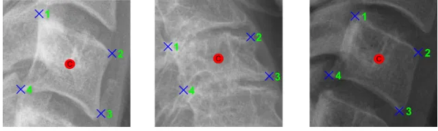
[image:3.612.151.471.533.629.2]90 lateral cervical spine X-ray images were collected from Royal Devon and Exeter Hospital in associ-ation with the University of Exeter. The age of the patients varied from 17 to 96. Different radiographic systems (Philips, Agfa, Kodak, GE) were used to produce the scans. Image resolution varied from 0.1 to 0.194 mm per pixel. The images include examples of vertebrae with fractures and degenerative changes. The data is anonymized and standard research protocols have been followed. For this work, 5 vertebrae C3-C7 are considered. Each of the 450 vertebrae from 90 images was manually annotated for corners and centers by an expert radiographer. Three annotated vertebrae are shown in Fig. 1.
Figure 1: Vertebra corners (x) and centers (o)
2.2. Hough Forest
2.2.1. Overview
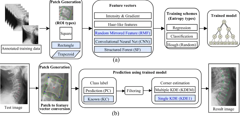
of five different types of feature vectors including a novel feature vector named random mirrored feature (RMF) (Sec. 2.2.4). Training is performed by Hough forest where both classification and regression en-tropy are used together. This training scheme has also been compared against standard training schemes, i.e. using either classification or regression entropy (Sec. 2.2.3). The training process is summarized in Fig. 2a where all the options available for each stage are shown graphically. Once the forests are trained, the framework can be used to predict corners for the new vertebrae. At test time, a new image is pro-vided with manually clicked vertebra centers. The ROIs are generated and patches are fed into trained forests, which then goes through a three stage process to localize corners: class prediction, filtering and corner estimation. The class prediction method has been improved by using prior knowledge from patch generation and corner estimation stage has been improved by using a cost efficient single kernel density estimation method (Sec. 2.2.5). The test time process is summarised as a flowchart in Fig. 2b.
Figure 2: (a) Training (b) Test flowcharts. Shaded block represents improvements and highlighted text represent novel contributions.
2.2.2. Patch Creation
The first step of the framework is to divide the vertebra into smaller patches. In order to do that, first, an ROI needs to be created around the vertebra centers. The position, overall size and orientation of this ROI can be calculated from the manually annotated vertebrae centers [1, 2]. In previous work [1, 2], a square ROI was constructed. However, distribution of the corners around the center for each vertebra reveals that vertebrae corners form a quadrilateral, that can be better approximated as a rectangle or trapezoid, as demonstrated in Fig. 3 which superimposes normalised corner distributions of the different cervical vertebral bodies in the dataset.
-0.5 0 0.5
-0.8 -0.6 -0.4 -0.2 0 0.2 0.4 0.6
Vertebra C3
-0.5 0 0.5
-0.8 -0.6 -0.4 -0.2 0 0.2 0.4 0.6
Vertebra C4
-0.5 0 0.5
-0.8 -0.6 -0.4 -0.2 0 0.2 0.4 0.6
Vertebra C5
-0.5 0 0.5
-0.8 -0.6 -0.4 -0.2 0 0.2 0.4 0.6
Vertebra C6
-0.5 0 0.5
-0.8 -0.6 -0.4 -0.2 0 0.2 0.4 0.6
[image:4.612.110.515.241.437.2]Vertebra C7
Figure 3: Normalized corner distribution in the dataset.
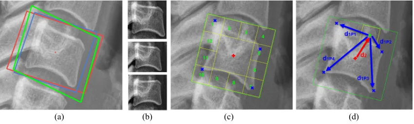
[image:4.612.89.538.596.677.2]The ROI is then divided in 16 equal-sized non-overlapping patches. Four center patches are discarded due to their homogeneous intensity distribution. Each of the boundary patches is associated with a class label (from 1 to 12) and five vectors. The class label (Cpatch) represents the position of the patch within the ROI and 4 vectors (d1P1,d1P2,d1P3andd1P4) point to four corners from the patch center and vector (d2) points to the vertebra center, as shown in Fig. 4. These image patches are converted to a feature vector (see Sec. 2.2.4) and fed into a Hough forest algorithm for training.
(a) (b) (c) (d)
Figure 4: (a) Different ROIs: Square (Blue), Rectangle (Red), Trapezoid (Green) (b) Vertebra inside different ROI: Square (Top), Rectangle (Middle), Trapezoid (Bottom) and Patches: (c) Class labels and (d) Vectors.
2.2.3. Training
Hough forest [17], a variant of the random forest [18, 19] algorithm, has shown promising performance in object detection using votes from image patches. Here this algorithm has been adapted and customized in order to localize vertebral corners in X-ray images. In contrast to the random forest algorithm which performs either regression or classification, Hough forest performs both together in the same forest. During training the algorithm requires training data, each of which is associated with a class label and a vector. In our case, patches generated from the vertebrae are converted into feature vectors (see Sec. 2.2.4). These feature vectors are considered as training data and corresponding class labels (Cpatch) and vectorsd1 are used to calculate the information gain (IG) using classification entropy (Hclass) or regression entropy (Hreg). The choice of entropy at each node is random for Hough forest. However, experiments have been conducted with pure classification and regression forest as well. The data flows down the tree until the maximum tree depth (D) is reached or number of elements in a node falls below a threshold (nM in).
IG=H(S)− X
i{L,R}
|Si| S H(S
i) (1)
The IG is calculated using Eqn. 1, whereS is a set of examples arriving at a node and SL, SR are the data that travel left or right respectively. H(S) is the entropy of the dataS. It can be either classification entropy,Hclass or regression entropy,Hreg. These can be calculated as below:
Hclass(S) =−
X
cC
p(c)log(p(c)) (2)
whereC is the set of classes available at the considered node. In our caseC⊆ {1,2,3, ...,12}.
Hreg(S) = 1
2log((2πe) 2|Λ(D
1)|) (3)
[image:5.612.101.526.184.312.2]2.2.4. Feature vectors
After creation, in order to train or test, the patches are converted into feature vectors. In this work, along with previously used feature vectors of [1, 2], we have considered and evaluated three other feature vectors including a novel one.
Intensity and gradient distribution-based feature vectors: The patches contain grey level intensity distributions (I). Patch sizes in pixels vary from image to image based on the corresponding X-ray resolution. In order to generate feature vectors of similar length and distributions range, patches are resized to form a square shape and distributions are normalized. Four sizes are considered: 30×30, 10×10, 5×5, and 3×3. These resized patches are then converted into feature vectors of dimension 900 (I30), 100 (I10), 25 (I5) and 9 (I3) respectively. The same procedure is repeated with the gradient distribution of each patch. Gradients are calculated in horizontal and vertical direction. Then the root-mean-square (RMS) of the magnitudes are considered. This also produced feature vectors of dimension 900 (G30), 100 (G10), 25 (G5) and 9 (G3). A few examples of the resized patches for intensity and gradient distributions are shown in Fig. 5. These feature vectors have been used in our previous work [1].
Intensity Gradient
[image:6.612.157.468.281.400.2]I30 I10 I5 I3 G30 G10 G5 G3
Figure 5: Appearance of intensity and gradient patches of different sizes
f f f f f
f f f f f
1 2 3 4 5
6 7 8 9 10
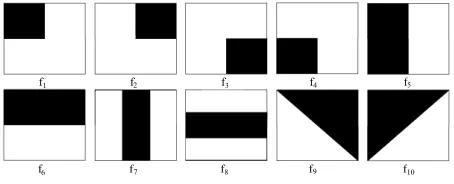
Figure 6: Haar-like feature templates
Haar-like feature vectors: Haar-like fea-tures have been used in numerous image process-ing approaches since its inception in [20]. For our work, ten Haar-like templates are chosen based on the patch appearances in terms of intensity and gradient distribution (see Fig. 6). Each template returns a feature value when passed through an intensity or gradient patch based on the differ-ence between the average intensity of the dark and bright area. Finally, feature vectors (Hv) are formed by the feature values from ten feature tem-plates.
fi= ¯Idark−I¯bright (4)
Hv= [f1, f2, f3, ..., f10] (5)
where ¯Ixis the average intensity of area denoted byx. Both intensity and gradient distributions are used to create two versions of Haar-like feature vectors of dimension ten: Haar-Intensity and Haar-Gradient. Another longer feature vector of dimension 20 has also been considered by putting both features together: Haar-Mixed. These feature vectors also have been investigated in our previous work [2].
[image:6.612.312.539.440.532.2]value is created from one pair by calculating the difference between the intensities (I) at those vector locations.
fi =I(d2+L1δ1)−I(d2+L2δ2) (6)
Figure 7: RMF
During training, a number (see Table 1) of feature values are com-puted at a split node and the one that maximises the information gain is chosen. This feature vector is inspired by the work of [21], where random displacement feature vectors are used in 3D on depth im-ages. In this work, two types of RMF are used. One that con-siders only one pixel at each of the random vector locations (RMF-1P) other that considers the average intensity of 3×3 pixel box cen-ter at each vector location (RMF-B) to calculate the feature values using Eqn. 6.
Convolutional Neural Net (CNN) feature vectors: Recently, convolutional neural networks (CNN) have shown impressive performance in a variety of machine learning and image analysis tasks. Off-the-shelf CNN feature vectors using a pre-trained deep network have been used for various compli-cated image processing tasks with great success [22]. Based on these recent developments, in this work, a pre-trained deep network (ImageNet-MatConvNet) is used to convert the patches into CNN feature vectors [23, 24]. Two different sizes of patches are considered for CNN feature vectors. The standard non-overlapping patch size inside the ROI generates CNN-S feature vector. Another larger and overlap-ping patch size is considered in order to provide more spatial information about the patch to the network, this feature vector is denoted by CNN-B. This size of the larger patch is the same asLmaxused for RMF feature vectors. The used deep network has 37 layers including the final classification layer. For this work, the response of 36th layer is used as the feature vector. A detailed description of this pretrained network can be found in [23]. This network requires a 3 channel RGB image of size 224×224 as an input. To achieve this our patches (both standard and larger) are resized to 224×224 and same grey-level intensity channel is repeated in each of the three channels. The dimension of the resultant feature vector is 1000.
Structured forest (SF) feature vectors: Edge detection is a fundamental problem in image processing. State-of-the-art works [25–27] on this field have shown significant improvement from the baseline [28]. All these recent papers use a complex feature vector. In order to compute the response vector from a patch, first, it is resized to a dimension of 16×16. Then gradient magnitude is computed in two scales (original and half down-sampled). For each scale, gradient orientations are computed with four directions resulting in 8 orientation channels. These 8 orientation channels, 2 magnitude channels and the original intensity channel (total 11) of size 16×16 are then resized to 5×5. These smaller size patches are then used to compute pair-wise difference vectors. 11 channels of size 16×16 results in 2816 feature candidates and pair-wise difference from same number of channels results in (11×5×5C
2=) 3300 feature candidates from each patch. The total feature dimension stands at 6116 from a single patch. Both patch sizes are considered to compute this vector: features computed from standard size patch is denoted by SF-S and larger patch is denoted as SF-B.
2.2.5. Prediction
At the time of testing, image patches from unseen vertebra are fed into the forest. Each patch travels through each tree and reaches a leaf node. Each leaf node contains vectord1s and class labels Cpatch of the examples present at that node. In [1, 2], the prediction stage first predicts the class of the image patch along with corner positions. However, as the image patches are created in a fixed manner based on the ROI, this class,Cpatch, is known at test time. In this work, along with the predicted class (PC) procedure of [1, 2], a new method has been formulated where known class (KC) of the patches are utilised. Class prediction in PC methods ˆCP C are computed by Eqn. 7 and on the other hand, ˆCKC is the class of the patch known at the time of its creation from the ROI.
ˆ
CP C= ˆCf orest= arg max ˆ Ctree
ˆ Cpatch=
(
ˆ
CP C for predicted class (PC) method, ˆ
CKC =Cpatch for known class (KC) method.
(8)
Once the class label ˆCpatch is determined, a filtering stage is introduced to discard all the d1 vectors belonging to classes other than ˆCpatch. These filteredd1s are then combined with the correspondingd2 of that patch to find the corner location with respect to the vertebra centre (see Fig. 4d). Then the final corner positiond is predicted using a single two-dimensional kernel density estimation (KDE1) process over the collection of vectors coming from all the patches. Previously in [1, 2], multiple KDEs were used to aggregate votes from leaf nodes (KDEM).
ˆ
d1tree= ˆd1f iltered={∀d1|c= ˆCpatch} (9)
ˆ
dpatch ={dˆ1tree(1),dˆ1tree(2), ...,dˆ1tree(N)} − {dˆ2patch,dˆ2patch, ...,dˆ2patch} (10)
ˆ
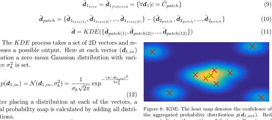
[image:8.612.97.539.214.409.2]d=KDE({dˆpatch(1),dˆpatch(2), ...,dˆpatch(12)}) (11)
Figure 8: KDE: The heat map denotes the confidence of
the aggregated probability distributionp(d1out). Red
crosses indicates the positions of the input d1 vector and
green circle represents the maxima ofp(d1out) and
out-put vectord1out.
TheKDEprocess takes a set of 2D vectors and re-gresses a possible output. Here at each vector (d1in) location a zero mean Gaussian distribution with vari-anceσ2
k is set.
p(d1in) =N(d1in, σk2) = 1
σk
√
2πexp
−(x−d1in)2 2σ2
k
(12) After placing a distribution at each of the vectors, a final probability map is calculated by adding all distri-butions.
p(d1out) = 1 n
n
X
i=1
pi(d1in) (13)
Finally, the maxima of this aggregated distribution are located and considered as the output vector (d1out). The process is also graphically summarized in Fig. 8.
2.3. Harris based vertebral corner detector
The Harris corner detector is a popular method to identify corners. It uses a second moment ma-trix composed of image derivatives. As with other gradient-based methods, it suffers if the image has low contrast, common to X-ray images. Initially, we attempted to compare our method to a standard implementation of the Harris corner detector, but results were poor due to lack of contrast. Therefore, we devised a novel multi-scale Harris corner detector-based framework with a spatial term trained from our manually labelled corners. Given a cervical X-ray image, similar to Sec 2.2.2, manually annotated vertebra centers are used to cut out an ROI around the vertebra. This ROI can be square, rectangle or trapezoid. This ROI is then passed through a collection edge detectors. In this work, Canny edge detector, Sobel, Prewitt, Roberts operators and Laplacian of Gaussian (LoG)-based edge detector are used. Each of these detectors returns a binary image. Then all the returned binary images are added together and an edge is determined only when more than two edge detectors agree. This process reduces noise and false edge detection.
EIψ=EdgeImage(ROI, ψ) (14)
whereψis the edge detection method: ψ {Canny, Sobel, Prewitt, Roberts, LoG};
EI =EICanny+EIP rewitt+EIRoberts+EILoG; (15)
Output Edge Image, EIO=
(
0 when EI<3,
1 otherwise. (16)
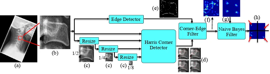
corner, the intensity profile at different scales increase the chance of detecting actual corners. Along with the corner location, it also returns a score which represents confidence of the detected corner. From each scale, the top 50 corners are selected. All the selected corners are then passed through a Corner-Edge filter where only the corners near edges (EIO= 1) are selected. Then these selected corners are converted into a probability distribution,P(C|I). A spatial prior probability distribution,P(L|I), is created from the training data containing all the corners (Fig. 3) except for the test image for that vertebra. These P(L|I) looks like Fig. 9g for different vertebrae. TheseP(L|I) is then made corner specificP(Li|I) by considering single (i-th) corners only. A final posterior distribution, P(Ci, Li|I) is then computed by multiplyingP(C|I) and P(Li|I) following a naive Bayes method. Final corner positions are found by localizing the maximum probability in each of the four posterior distributionP(Ci, Li|I). The complete framework is graphically explained in Fig. 9.
P(Li|I) = 1 N
N
X
j=1 1
σc
√
2πexp
−(x−2Cijσ2)2
c , (17)
where N is the number of training examples,σ2c is the variance of Gaussian distribution initialized at each training corner locations andP(Li|I) is the prior probability distribution for i-th corner. The variance, σc2, is optimized experimentally using a set of test images.
P(Ci, Li|I) =P(C|I)×P(Li|I), (18) whereCi is the i-th corner, Li is the location of that corner, and I is the ROI. P(C|I) comes from the edge-filtered multi-scale Harris corner detection andP(Li|I) comes from training data.
(a)
(b)
(c) (c) (c) (d)
(e)
(f) (g) (h)
Edge Detector
Resize Resize
Resize
Harris Corner Detector
Corner-Edge
Filter Naive BayesFilter
1/2
1/4
[image:9.612.89.538.386.510.2]1/8
Figure 9: Harris based vertebra corner detector (a) Original X-Ray (b) cropped ROI (c) ROI at different scales (d) Harris
Corner detector output at each scale (e) Binary edge image (EIO) (f) Output of Corner-Edge filter: P(C|I) (g)P(L|I) (h)
final distribution:P(C, L|I), corners are pointed out by red arrows.
3. Parameters
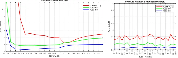
There are a few free parameters in the corner localization forests: number of trees (nTree), maximum allowed depth of a tree (D), minimum number of elements at a node (nMin), number of variables to look at in each split nodes (nVar) and number of thresholds (nTresh) to consider per variable. Apart from the random forest parameters, the kernel density estimation function requires a given bandwidth (BW) which is the variance,σ2
and annotated manually by experts for the fixed test set. Two example of error vs. parameter value graphs are plotted for BW selection and nVar-nTheta selection for Haar-Mixed features is shown in Fig. 10. The BW selection graph indicates that the lowest error occurs with BW = 0.03 for KDE1+KC method. Lowest error for nVar-nTheta selection occurs at 2-1. The next option could have been 4-5, but that would increase the computational cost by a factor of ten. Similarly, all the parameters are optimized based on the lowest error and corresponding computational cost. The chosen parameters are reported in Table 1.
Bandwidth
0.0010.005 0.01 0.02 0.03 0.04 0.05 0.06 0.07 0.08 0.09 0.1 0.2 0.3 0.4 0.5 0.6 0.7 0.8 0.9 1
Error in MM
1.5 2 2.5 3 3.5 4 4.5 5
Bandwidth (BW) Selection
KDEM+PC [2] KDE1+PC KDE1+KC
nVar - nTheta
1 - 1 1 - 2 1 - 5 1 - 10 1 - 20 2 - 1 2 - 2 2 - 5 2 - 10 2 - 20 3 - 1 3 - 2 3 - 5 3 - 10 3 - 20 4 - 1 4 - 2 4 - 5 4 - 10 4 - 20 5 - 1 5 - 2 5 - 5 5 - 10 5 - 20
Error in MM
1.5 2 2.5 3 3.5 4 4.5 5
nVar and nTheta Selection (Haar Mixed)
KDEM+PC [2] KDE1+PC KDE1+KC
Figure 10: Bandwidth (BW), Number of variables (nVar) and number of thresholds (nThresh) selection.
Table 1: Optimized parameters for corner localization
Parameters Features Dimension Value
BW (σ2k)
ALL
0.03
nTree 100
D 10
nMin 5
nVar - nThresh
SF 6116
85-10
RMF Infinity* (5000)
CNN 1000 30-10
I30 900 15-20 G30 I10 100 10-2 G10 I5 25 2-1 G5
Haar Mixed 20
I3 9 1-5 G3 Haar Intensity 10 Haar Gradient
The rest of the experiments are conducted with these parameter values. (*RMF is dynamically created with random vectors so technically feature dimension is infinity, however for the sake of implementation, the choice of possible vector locations was quantized such that maximum possible feature dimension becomes 5000.)
4. Experiments & Results
4.1. Effect of different ROIs
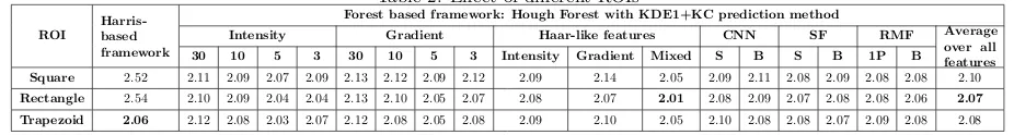
Both the Harris corner detector-based framework and the forest-based framework are experimented with three ROI types: square, rectangle and trapezoid; results shown in Table 2. (The forest framework results here are for Hough (random entropy selection) forest type and with KDE1+KC prediction type). The Harris framework shows an increase in error from square to rectangle ROI and a sharp decrease for the trapezoid ROI. The increased area of a rectangle from the square sometimes triggers false corners whereas for a trapezoid, the axis-aligned edges results in much better edge and corner detection and decreases the error to 2.06 mm. A different pattern is observed for the forest-based framework. The results for square and rectangle ROIs are always (for all features) better than the Harris framework but in the case of the trapezoid, the results are very comparable. The average over all the features show that the rectangle and trapezoid ROI performs marginally better than square, and in between these two, the rectangle is slightly better. However, the pattern is not consistent with all the features. The lowest error of 2.01 mm is achieved with the Haar-Mixed feature for the rectangle ROI. The Harris framework clearly shows that the trapezoid ROI can help when the algorithm uses horizontal and vertical gradients to detect edges and corners as this ROI aligns the vertebra edges (see Fig. 4b). But the forest framework does not directly use this information thus the differences are not noticeable. Among all the features Haar-Mixed performed the best followed by Intensity 5 (I5). The advanced features (RMF, CNN, SF) do not perform very well in terms of the error.
Table 2: Effect of different ROIs
ROI
Harris-based framework
Forest based framework: Hough Forest with KDE1+KC prediction method
Intensity Gradient Haar-like features CNN SF RMF Average
over all features
30 10 5 3 30 10 5 3 Intensity Gradient Mixed S B S B 1P B
Square 2.52 2.11 2.09 2.07 2.09 2.13 2.12 2.09 2.12 2.09 2.14 2.05 2.09 2.11 2.08 2.09 2.08 2.08 2.10
Rectangle 2.54 2.10 2.09 2.04 2.04 2.13 2.10 2.05 2.07 2.08 2.07 2.01 2.08 2.09 2.07 2.08 2.08 2.06 2.07 Trapezoid 2.06 2.12 2.08 2.03 2.07 2.12 2.08 2.05 2.08 2.09 2.10 2.05 2.10 2.08 2.08 2.07 2.09 2.08 2.08
4.2. Comparison of forest type
[image:11.612.80.543.337.399.2]Table 3: Performance of different forest types (Errors)
Forest type
Forest framework with KDE1+KC prediction method (Rectangle ROI)
Intensity Gradient Haar-like CNN SF RMF
Average 30 10 5 3 30 10 5 3 Intensity Gradient Mixed S B S B 1P B
Regression 2.10 2.08 2.05 2.07 2.10 2.08 2.06 2.05 2.08 2.06 2.02 2.11 2.10 2.10 2.11 2.09 2.09 2.08
Classification 2.04 2.05 2.03 2.05 2.15 2.14 2.06 2.11 2.05 2.14 2.03 2.08 2.12 2.05 2.07 2.06 2.04 2.0748
Hough 2.10 2.09 2.04 2.04 2.13 2.10 2.05 2.07 2.08 2.07 2.01 2.08 2.09 2.07 2.08 2.08 2.06 2.0726
Table 4: Performance of different forest types (% of Patch Classification Accuracy)
Forest type
Forest framework with KDE1+KC prediction method (Rectangle ROI)
Intensity Gradient Haar-like CNN SF RMF
Average
30 10 5 3 30 10 5 3 Intensity Gradient Mixed S B S B 1P B
Regression 9.46 40.68 56.47 53.57 8.78 24.47 41.29 39.88 48.09 35.92 53.56 9.63 9.41 10.03 11.99 9.14 9.50 27.76
Classification 61.56 61.87 58.85 57.25 32.75 42.25 44.14 43.38 51.28 39.50 55.25 47.55 42.58 71.50 92.40 84.06 85.38 57.15 Hough 54.71 56.99 57.47 56.31 25.08 38.68 43.20 42.88 50.51 38.48 54.41 43.25 37.21 66.11 90.92 80.37 82.04 54.04
is not trained with any X-ray images. Also, the used network is trained to accomplish a highly complex task of classifying an image into certain classes based on the content of the image like- dog, cat, bicycle etc. In our case, the image patches are not complex, rather it is just a grey level distribution having one edge and/or corner and often with very low contrast. One solution could be to use only first few layers of the network which are usually responsible to detect simple gradient features of different types. Alternatively, one could train a new network with the corresponding data.
4.3. Per-vertebra analysis
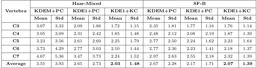
[image:12.612.100.520.519.630.2]To compare between three prediction methods (KDEM+PC, KDE1+PC and KDE1+KC), the best feature in terms of errors, Haar-Mixed and the best feature in terms of patch classification accuracy, SF-B are considered. Table 5 lists vertebra by vertebra mean and standard deviation (std) of the errors (over 90 images and 4 corners) for two features and three prediction type (with classification forest and rectangle ROI). The corner-by-corner mean errors are also plotted in Fig. 11. It can be observed that for all the features and prediction types, the error tends to increase as it moves down the spine from C3 to C7. Among three prediction methods, the graph in Fig. 11 and also Fig. 10 clearly indicates that KDE1+KC is the most robust and performs the best. Followed by KDE1+PC and KDEM+PC [2]. However, both KDE1+PC and KDE1+KC perform comparably well in the case of SF-B feature. This is because of the excellent patch classification accuracy achieved by this feature.
Table 5: Average error of different vertebra
Vertebra
Haar-Mixed SF-B
KDEM+PC KDE1+PC KDE1+KC KDEM+PC KDE1+PC KDE1+KC
Mean Std Mean Std Mean Std Mean Std Mean Std Mean Std
C3 3.07 3.33 2.09 1.86 1.72 1.15 2.35 1.81 1.77 1.16 1.76 1.14
C4 3.05 3.09 2.31 2.42 1.85 1.48 2.48 2.12 2.08 2.19 1.87 1.39
C5 3.23 3.56 2.61 2.60 2.25 1.79 2.77 2.50 2.24 1.62 2.23 1.64
C6 3.73 4.29 2.77 3.03 2.10 1.44 2.77 2.36 2.23 1.41 2.18 1.37
C7 4.67 5.36 3.47 3.73 2.24 1.52 2.97 2.63 2.55 2.18 2.32 1.39
Average 3.55 3.93 2.65 2.73 2.03 1.48 2.67 2.28 2.17 1.71 2.07 1.39
4.4. Discussion
Vertebra - Corner
C3-1 C3-2 C3-3 C3-4 C4-1 C4-2 C4-3 C4-4 C5-1 C5-2 C5-3 C5-4 C6-1 C6-2 C6-3 C6-4 C7-1 C7-2 C7-3 C7-4
Mean error in MM
1.5 2 2.5 3 3.5 4 4.5
5 Error pattern over vertebrae
[image:13.612.178.441.97.243.2]Haar-Mixed KDEM+PC Haar-Mixed KDE1+PC Haar-Mixed KDE1+KC SF-B KDEM+PC SF-B KDE1+PC SF-B KDE1+KC
Figure 11: Mean error pattern over vertebra corners
reflecting a 33% improvement over [2]. Among other work, Glocker et al. [9] reported a mean error of 6 mm in locating vertebra centers in CT images. Zamora et al. [15] reports a mean corner to segmentation line error of higher than 3 mm, whereas, for our algorithm, point to point error for corners is found to be only 2.01 mm. Representative results on the vertebrae are shown in Fig. 12. Unsurprisingly, our forest based algorithm suffers when a test image is not similar to any the training images (Fig. 12(C6-E) - longer bone structure). Sometimes some patients have implants or severe degenerative change that renders corner detection a difficult problem. However, the strength of this framework is that through the vote aggregation procedure from different patches, a robust result can be achieved even if some patches are noisy or occluded (Fig. 12(C5-D)).
C3
C4
C5
C6
C7
A B C D E
[image:13.612.131.492.387.739.2]5. Conclusion
Two vertebral corner detection frameworks have been studied in this work. The Hough forest frame-work of [1, 2] has been improved with data-driven ROI generation (rectangle and trapezoid) and advanced, simpler corner localization method (KDE1). Along with the previous features of [2], more advanced and complex features like CNN and SF features are considered. A novel feature, RMF, is introduced which performed considerably well in terms of patch classification accuracy. On the other hand, a novel Har-ris corner detector-based framework has also been formulated. This framework achieved a lowest error of 2.06 mm with trapezoid ROI outperforming many features in forest-based framework. However, the overall lowest error of 2.01 mm is achieved by Haar-Mixed feature with rectangle ROI and Hough forest. Along with the corner localization error, patch classification accuracy has also been investigated where SF feature achieved a maximum accuracy of 92.4% with classification forest and rectangle ROI.
The current framework requires manually clicked seed points (vertebra centers) at test time. We have already demonstrated a global spine localization algorithms in [6] which could be further developed to localize vertebra centers. By combining these two algorithms, a fully automatic vertebral corner detection method can be formulated. In future work, these predicted corners will be used to initialise an ASM for segmentation of the vertebra. Once initialized correctly using predicted corners, the ASM is expected to segment the vertebra more accurately than an initialization based solely on the vertebra centers.
References
[1] S. M. M. R. Al-Arif, M. Asad, K. Knapp, M. Gundry, and G. Slabaugh, “Hough forest-based corner detection for cervical spine radiographs,” in Medical Image Understanding and Analysis (MIUA), Proceedings of the 19th Conference on, pp. 183–188, 2015.
[2] S. M. M. R. Al-Arif, M. Asad, K. Knapp, M. Gundry, and G. Slabaugh, “Cervical vertebral corner detection using Haar-like features and modified Hough forest,” in Image Processing Theory, Tools and Applications (IPTA), 2015 5th International Conference on, IEEE, 2015.
[3] P. Platzer, N. Hauswirth, M. Jaindl, S. Chatwani, V. Vecsei, and C. Gaebler, “Delayed or missed diagnosis of cervical spine injuries,” Journal of Trauma and Acute Care Surgery, vol. 61, no. 1, pp. 150–155, 2006.
[4] C. Morris and E. McCoy, “Clearing the cervical spine in unconscious polytrauma victims, balancing risks and effective screening,”Anaesthesia, vol. 59, no. 5, pp. 464–482, 2004.
[5] A. Tezmol, H. Sari-Sarraf, S. Mitra, R. Long, and A. Gururajan, “Customized hough transform for robust segmentation of cervical vertebrae from x-ray images,” inImage Analysis and Interpretation, 2002. Proceedings. Fifth IEEE Southwest Symposium on, pp. 224–228, IEEE, 2002.
[6] S. M. M. R. Al-Arif, M. Gundry, K. Knapp, and G. Slabaugh, “Global localization and orientation of the cervical spine in x-ray images,” inComputational Methods and Clinical Applications for Spine Imaging (CSI), The Fourth MICCAI Workshop on, Springer, 2016.
[7] T. Klinder, J. Ostermann, M. Ehm, A. Franz, R. Kneser, and C. Lorenz, “Automated model-based vertebra detection, identification, and segmentation in ct images,”Medical Image Analysis, vol. 13, no. 3, pp. 471–482, 2009.
[8] X. Dong and G. Zheng, “Automated vertebra identification from x-ray images,” inImage Analysis and Recognition, pp. 1–9, Springer, 2010.
[9] B. Glocker, J. Feulner, A. Criminisi, D. R. Haynor, and E. Konukoglu, “Automatic localization and identification of vertebrae in arbitrary field-of-view CT scans,” in Medical Image Computing and Computer-Assisted Intervention–MICCAI 2012, pp. 590–598, Springer, 2012.
[11] M. Benjelloun, S. Mahmoudi, and F. Lecron, “A framework of vertebra segmentation using the active shape model-based approach,”Journal of Biomedical Imaging, vol. 2011, p. 9, 2011.
[12] S. M. M. R. Al-Arif, M. Gundry, K. Knapp, and G. Slabaugh, “Improving an active shape model with random classification forest for segmentation of cervical vertebrae,” inComputational Methods and Clinical Applications for Spine Imaging (CSI), The Fourth MICCAI Workshop on, Springer, 2016.
[13] T. F. Cootes, C. J. Taylor, D. H. Cooper, and J. Graham, “Active shape models-their training and application,”Computer Vision and Image Understanding, vol. 61, no. 1, pp. 38–59, 1995.
[14] T. F. Cootes, G. J. Edwards, and C. J. Taylor, “Active appearance models,”IEEE Transactions on Pattern Analysis & Machine Intelligence, no. 6, pp. 681–685, 2001.
[15] G. Zamora, H. Sari-Sarraf, and L. R. Long, “Hierarchical segmentation of vertebrae from x-ray images,” in Medical Imaging 2003, pp. 631–642, International Society for Optics and Photonics, 2003.
[16] M. G. Roberts, T. F. Cootes, and J. E. Adams, “Automatic location of vertebrae on dxa images using random forest regression,” inMedical Image Computing and Computer-Assisted Intervention– MICCAI 2012, pp. 361–368, Springer, 2012.
[17] J. Gall, A. Yao, N. Razavi, L. Van Gool, and V. Lempitsky, “Hough forests for object detection, tracking, and action recognition,” Pattern Analysis and Machine Intelligence, IEEE Transactions on, vol. 33, no. 11, pp. 2188–2202, 2011.
[18] L. Breiman, “Random forests,”Machine Learning, vol. 45, no. 1, pp. 5–32, 2001.
[19] A. Criminisi and J. Shotton, Decision forests for computer vision and medical image analysis. Springer Science & Business Media, 2013.
[20] P. Viola and M. Jones, “Rapid object detection using a boosted cascade of simple features,” in Com-puter Vision and Pattern Recognition, 2001. CVPR 2001. Proceedings of the 2001 IEEE ComCom-puter Society Conference on, vol. 1, pp. I–511, IEEE, 2001.
[21] J. Shotton, T. Sharp, A. Kipman, A. Fitzgibbon, M. Finocchio, A. Blake, M. Cook, and R. Moore, “Real-time human pose recognition in parts from single depth images,”Communications of the ACM, vol. 56, no. 1, pp. 116–124, 2013.
[22] A. S. Razavian, H. Azizpour, J. Sullivan, and S. Carlsson, “CNN features off-the-shelf: an astounding baseline for recognition,” inComputer Vision and Pattern Recognition Workshops (CVPRW), 2014 IEEE Conference on, pp. 512–519, IEEE, 2014.
[23] K. Simonyan and A. Zisserman, “Very deep convolutional networks for large-scale image recognition,” arXiv preprint arXiv:1409.1556, 2014.
[24] “MatConvNet.”http://www.vlfeat.org/matconvnet/. Accessed: 2016-11-04.
[25] P. Doll´ar and C. L. Zitnick, “Structured forests for fast edge detection,” inProceedings of the IEEE International Conference on Computer Vision, pp. 1841–1848, 2013.
[26] P. Doll´ar and C. L. Zitnick, “Fast edge detection using structured forests,”IEEE Transactions on Pattern Analysis and Machine Intelligence, vol. 37, no. 8, pp. 1558–1570, 2015.
[27] S. Hallman and C. C. Fowlkes, “Oriented edge forests for boundary detection,” inProceedings of the IEEE Conference on Computer Vision and Pattern Recognition, pp. 1732–1740, 2015.