Novel Method for State Space Modeling of Full Bridge Converter

Abstract: The requirement of converters is increasing with the increase in demand for the power conversion devices. For efficient power conversion, stability and time response of the system must be improved. For improving characteristics a mathematical model of the system must be determined. In this paper, an improvised state space model of full bridge converter is presented which can be used in converter design. This state-space model incorporates the non-idealities of the transformers like discharge time of primary inductance and secondary inductance as well as the wire resistance. The interdependency of the parameters affects the state space model of the converter compared to the ideal modeling. This variation in state space model of the converter has an impact on design of compensator which improves the system efficiency of the converter.

Keywords : State Space Representation, Discharge time Primary Inductance, Secondary Inductance.

I.INTRODUCTION

D

C-DC converters are implemented as an interface between the power source and appliance as to ensure compatibility between the power supply provided and the connected load. DC-DC converters are of two categories; isolated converters and isolated converters. The non-isolated topologies include buck, boost, buck-boost and other configurations of these converters. The isolated topologies include flyback, forward, push-pull, half bridge and full bridge converter.

In case of high power requirements the recommended DC-DC converter is full bridge converter (for example in battery charger of an electric vehicle). To ensure a better output, switching must be controlled as per the variations in the load, hence a closed loop operation is required for switching and hence controller is required which can generate precise PWM pulses. Methods to determine control parameters of the controller are: 1.) Determining the transfer function by conventional methods i.e. using Laplace transformation. 2.) Determining the state space model. The transfer function of the system can also be found by state space model in the zero-pole-gain form [1]. Through the transfer function approach the parameters can be evaluated using Bode plots or root-locus which determines the poles and zeros. The control parameters can also be obtained by using the state-space representation directly using the observability criteria[2].

Revised Manuscript Received on October 05, 2019. * Correspondence Author

Aniruddh Kulkarni, Undergraduate Student, Institute of Technology, Nirma University, Ahmedabad, 382481, Gujarat, India. Email: [email protected]

P. N. Kapil*, Assistant Professor, Institute of Technology, Nirma University, Ahmedabad, 382481, Gujarat, India, [email protected]

State space representation is a mathematical model of a system in which the parameters of the system are expressed in matrix form in a unique combination[2]. The generic representation of the state space model can be given as:.

[𝑑𝑥/𝑑𝑡] = [𝐴] ∗ [𝑥] + [𝐵] ∗ [𝑢]

(1)

[𝑦] = [𝐶] ∗ [𝑥] + [𝐷] ∗ [𝑢]

(2)

Here,

𝑥

= State variable matrix

𝑢

= Input matrix

𝑦

= Output matrix

The matrices [A], [B], [C], [D] represent scaling matrices which consists of the constants that are multiplied to the state parameters and the input parameters so as to satisfy the circuit equations.

[𝐴]

= System-State matrix

[𝐵]

= Input matrix

[𝐶]

= Output matrix

[𝐷]

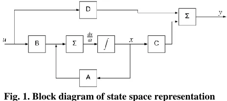
= Feed-Forward Matrix

[image:1.595.315.547.449.552.2]

The block diagram of state space representation which illustrates the parameters that contribute to the output and the order of the matrices is represented in figure 1[2].

Fig. 1. Block diagram of state space representation equations

II.RESEARCHMETHOD

The state-space technique is only applicable to LTI (Linear-Time-Invariant) systems. As seen from the equations the term

𝑑𝑥/𝑑𝑡

represents slope, which implies that the system must be linear and hence the operation of the model can be predicted. The term

𝑑𝑥/𝑑𝑡

holds no significance when the model contains non-linear parameters. Hence the circuit is linearised in order to obtain the mathematical model. The slope is determined by the storage elements in the circuit like the inductor and the capacitor.

𝐿𝑑𝑖/𝑑𝑡 = 𝑉

𝐶𝑑𝑉/𝑑𝑡 = 𝐼

These two equations represent the slope of the measured parameters which are the inductor current and the capacitor voltage.

Novel Method for State Space Modeling of Full

Bridge Converter

Hence the inductor current and the capacitor voltages are considered as state variables while obtaining model for a DC-DC converter.

A.Advantages of using state space for isolated topologies

The method of obtaining transfer function of isolated topologies is complex as the circuit involves transformer and switches. Hence a state space model is used to obtain the representation of such circuits.

The circuit of DC-DC converter contains different operating modes and the components of the circuit which are operating vary. Hence, the circuit contains linear components when segregated according to ON and OFF time periods.

B.Full Bridge Converter Operation

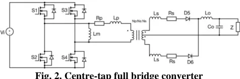
[image:2.595.51.289.316.395.2]

The full bridge converter with the equivalent circuit model of the isolation transformer is given in fig-2. The state space representation is completed by modelling the circuit in ON time and the OFF time. The switching of hard switched full bridge converter are given in four modes[3].

Fig. 2. Centre-tap full bridge converter

Mode 1: During the first mode the switches S1 and S4 are in

on state. The positive input voltage is applied across the primary winding of the transformer. The secondary of the transformer is centre-tap. Hence, for the positive voltage applied across the primary winding upper winding of the secondary of centre-tap transformer is in operating state.

Mode 2: In this mode the switches S1 and S4 are turned off

and the inductor freewheels across the secondary and the leakage inductance of the transformer on the primary discharges. The freewheeling mode is necessary as to ensure that the inductor is not saturated. On the secondary, both the diodes are active during freewheeling mode.

Mode 3: This mode is similar to Mode 1. In this mode the switches S2 and S3 are turned on. Hence, negative voltage is

applied across the primary winding and the lower winding of the secondary if centre-tap transformer is active. The direction of inductor current does not change.

Mode 4: This mode is same as Mode 2. The inductor discharges through the load and both the diodes remain in the on state during this mode. The current is equally divided in both the winding. Therefore, the current in each winding is 𝐼𝑠/2, where 𝐼𝑠 is the secondary current.

III.STATESPACEREPRESENTATION

The state space representation is modelled for all four modes individually and then the complete state space model is obtained by circuit averaging [3]. The magnetizing inductance is not considered as the high frequency transformer is not used for storing energy when used in

isolated converters [1]. Hence, the value of magnetizing inductance is selected to be sufficiently high and hence the current in the magnetizing path can be neglected as compared to the current in the leakage inductance. Therefore, the magnetizing inductance can be neglected. Here an assumption is made that, on the secondary side the leakage inductance and the filter inductance are added in order to achieve effective inductance (L). In the on state, only one of the diode is active. Hence, the effective inductance is the sum of secondary leakage inductance and the filter inductance. During the OFF time the filter inductance freewheels and hence the current is split into two equal halves at the centre-tap. The contribution of voltage drop of the leakage inductances is same for both. As the number of turns are the same on both the windings of secondary the leakage inductance remain same. As the voltage drops in both the inductances are halved as the current through the inductance is halved the net drop is equivalent to the on-state drop of one leakage inductance and hence the effective inductance can be represented by adding the filter inductance and the leakage inductance of any one part of the winding. Hence on the secondary side the storage elements are

𝐿

and

𝐶

_𝑜 which is the filter capacitance.

State Space Model can be determined by:

Step 1: Identifying the storage elements

On the primary side of the transformer the storage element is the leakage inductance

𝐿

₁. On the secondary side the storage elements are

𝐿

and

𝐶

_𝑜 where,

𝐿

1= Primary leakage inductance.

𝐿

= Sum of secondary leakage inductance and filter inductance.

𝐶

𝑜= Filter capacitor.

Step 2: Mentioning the state vectors, input vectors and the output vectors.

The matrix of state vectors consists of the parameters that the storage elements.

𝑥 =

𝑖

𝑙1

𝑖

𝑙

𝑣

𝐶0 ;

This is the state vector matrix.

where,

𝑖

_𝑙 is the current through the effective inductance

𝐿

.

𝑖

𝑙₁represents the current through the primary circuit.

𝑣

𝐶0 represents the voltage across capacitor.

𝑢 = 𝑣

𝑖 ; This is the input matrix, where

𝑉

𝑖 is the input voltage.

𝑦 = 𝑣

𝑜 ; This is the output matrix, where

𝑉

_𝑜 is the output voltage.

Step 3: State space model for on time (0 − 𝛼𝑇𝑠).

𝛼 =

𝑡𝑜𝑛

𝑡𝑜𝑓𝑓, where α represents the duty ratio.

𝑇

𝑠 represents the switching time.

𝑑𝑖_𝑙1 𝑑𝑡

=

𝑉𝑖−𝑖𝑝𝑅𝑝

𝑖

𝑙1 represents the current though the primary leakage inductance and

𝑖

𝑝 represents the current in the primary

circuit. But

𝑖

_𝑝

= 𝑖

_𝑙1 as the current in the transformer is in series with the leakage inductance. Hence the equation is now represented as,

𝑑𝑖_𝑙1 𝑑𝑡

=

𝑉𝑖−𝑖𝑙1𝑅𝑝 𝐿₁

=

−𝑖_𝑙1𝑅𝑝 𝐿₁

+

𝑉_𝑖

𝐿₁ (4) Here,

𝑅

𝑝 represents the net resistance on the primary side. This includes the on-state resistance of the switches, the winding resistance and the leakage resistance of the transformer.

The equations of the other space vectors can be written as,

𝑑𝑖𝑙 𝑑𝑡

=

𝑉𝑠−𝑖𝑠𝑅𝑠−𝑉𝑜

𝐿 (5) Aforementioned the value of

𝐿

can be evaluated by adding the leakage inductance of one of the windings and the filter inductance.

𝑅

_𝑠 represents the net resistance on the secondary side which incorporates the leakage resistance, winding resistance and on-state resistance of the diode.

𝐶𝑉

𝐶0

= 𝑄

𝑐, differentiating this equation yields, 𝑑𝑉_𝑐0

𝑑𝑡

=

𝑖_𝑐 𝐶₀

=

𝑖_𝑙 𝐶₀

−

𝑉_𝑜

𝑍∗𝐶₀ (6) where,

𝑍

represents the load impedance connected to the output of the converter.

Based on these three equations the state space matrix of the full bridge converter in the positive on state can be written in the format of

[𝑑𝑥/𝑑𝑡] = [𝐴

1

] ∗ [𝑥] + [𝐵

1

] ∗ [𝑢]

(7) 𝑑𝑖_𝑙1

𝑑𝑡 𝑑𝑖𝑙 𝑑𝑡 𝑑𝑣_𝐶0

𝑑𝑡

=

−𝑅𝑝

𝐿1

0

0

−𝑅𝑝∗𝑛𝑠 𝐿

−𝑅_𝑠 𝐿

−1 𝐿

0

1

𝐶0 −1 𝑍∗𝐶0

∗

𝑖

𝑙1

𝑖

𝑙

𝑣

𝐶0

+

1 𝐿1 𝑛_𝑠 𝑛_𝑝∗𝐿

0

∗ 𝑉

𝑖

(8)

[𝑦] = [𝐶

1

] ∗ [𝑥] + [𝐷

1

] ∗ [𝑢]

(9)

𝑉

0

= 0 0 1 ∗

𝑖

𝑙1

𝑖

𝑙

𝑣

𝐶₀

+ 0 ∗ 𝑉

𝑖

(10)

where

𝐴

1,

𝐵

1,

𝐶

1,

𝐷

1 represent the state matrices of obtained in mode 1. By comparing these equations the value of

𝐴

₁,

𝐵

₁,

𝐶

₁,

𝐷

₁ can be obtained.

Step 4: State space model for dead time(

𝛼𝑇

𝑠

− 𝑇

𝑠) The time interval during dead time is split into two parts. During the dead time the primary leakage inductor discharges. As the inductor discharges by reversing its polarity, the diodes of switches S2 and S3 turn on. This state

is similar to mode 3 in which the switches are turned on.

Hence, to model the circuit in dead time interval, it is divided into two parts:

1. Interval in which leakage inductor of transformer discharges (Mode 2.1).

2.Time interval when the transformer is off (Mode2.2). Hence, there are two state space model for the dead time interval. Evaluating part-wise,

Mode 2.1-When the leakage inductance discharges

Consider the time for which the leakage inductor discharges to be

𝑡

_𝑓

(1 − 𝛼)𝑇

_𝑠; where

𝑡

_𝑓 is a fraction of time

(1 −

𝛼)𝑇

𝑠 for which the inductor discharges. As this mode is similar to mode-3, the voltage across primary is

−𝑉

_𝑖. Hence the matrices of mode-3 and mode 2.1 will be same.

𝑑𝑖_𝑙1 𝑑𝑡

=

−𝑉𝑖+𝑖𝑝𝑅𝑝

𝐿1 (11) and

𝑖

_𝑝

= 𝑖

_𝑙1

Hence the equation can be written as, 𝑑𝑖_𝑙1

𝑑𝑡

=

𝑖𝑝𝑅𝑝

𝐿1

−

𝑉𝑖

𝐿1 (12)

The equation of the secondary side can be written will remain same as mode 1. As the secondary side has two diodes, if the negative voltage is applied on the primary side the diode on the other part of the winding is active but the equations remain same. The equation of the other state parameters are:

𝑑𝑖𝑙 𝑑𝑡

=

𝑉𝑠−𝑖𝑠𝑅𝑠−𝑉𝑜

𝐿 (13)

𝑑𝑉_𝐶0 𝑑𝑡

=

𝑖_𝐶0 𝐶0

=

𝑖𝑙 𝐶0

−

𝑉𝑜

𝑍∗𝐶0 (14)

Hence the state space model of the mode 2.1 can be written as,

[𝑑𝑥/𝑑𝑡] = [𝐴

2.1

] ∗ [𝑥] + [𝐵

2.1

] ∗ [𝑢]

(15)

𝑑𝑖_𝑙1 𝑑𝑡 𝑑𝑖_𝑙 𝑑𝑡 𝑑𝑣_𝐶0

𝑑𝑡

=

𝑅_𝑝

𝐿1

0

0

−𝑅𝑝∗𝑛𝑠 𝐿

−𝑅𝑠 𝐿

−1 𝐿

0

1

𝐶0 −1 𝑍∗𝐶0

∗

𝑖

𝑙₁

𝑖

𝑙

𝑣

𝐶0

+

−1 𝐿₁ 𝑛𝑠 𝑛𝑝∗𝐿

0

∗ 𝑉

𝑖

(16)

[𝑦] = [𝐶

2.1

] ∗ [𝑥] + [𝐷

2.1

] ∗ [𝑢]

(17)

𝑉

0

= 0 0 1 ∗

𝑖

𝑙1

𝑖

𝑙

𝑣

𝐶0

+ 0 ∗ 𝑉

𝑖

(18)

Mode 2.2: Time interval when the transformer is off. In this mode the value of

𝑖

_𝑙

1 is zero and as the leakage inductor has discharged the value of

𝑑𝑖

_𝑙1

/𝑑𝑡

is also 0. The equation of the other state parameters can be stated as,

𝑑𝑖_𝑙 𝑑𝑡

=

−𝑉_𝑜−𝑖_𝑠𝑅_𝑠

𝐿 (19)

The equation of capacitor remains same.

𝑑𝑣_𝐶0 𝑑𝑡

=

𝑖_𝐶0 𝐶₀

=

𝑖_𝑙 𝐶₀

−

𝑉_𝑜

𝑍∗𝐶₀ (20)

Hence the state matrix during the mode 2.2 can be written as,

[𝑑𝑥/𝑑𝑡] = [𝐴

2.2

] ∗ [𝑥] + [𝐵

2.2

] ∗ [𝑢]

(21) 𝑑𝑖_𝑙1 𝑑𝑡 𝑑𝑖𝑙 𝑑𝑡 𝑑𝑣_𝐶0 𝑑𝑡

=

0

0

0

0

−𝑅𝑠

𝐿 −1 𝐿

0

1 𝐶0 −1 𝑍∗𝐶0

∗

𝑖

𝑙₁

𝑖

𝑙

𝑣

𝐶₀

+

0

0

0

∗ 𝑉

𝑖

(22)

[𝑦] = [𝐶

2.2

] ∗ [𝑥] + [𝐷

2.2

] ∗ [𝑢]

(23)

𝑉

0

= 0 0 1 ∗

𝑖

𝑙1

𝑖

𝑙

𝑣

𝐶₀

+ 0 ∗ 𝑉

𝑖 (24)

where,

[𝐴

_2.2

]

,

[𝐵

_2.2

]

,

[𝐶

_2.2

]

,

[𝐷

_2.2

]

are state matrices for mode 2.2.

Mode 3: This mode is same as mode 2.1 and hence the state model for this mode can be written is same as mode 2.1. Therefore the state space model can be represented as,

[𝑑𝑥/𝑑𝑡] = [𝐴

3

] ∗ [𝑥] + [𝐵

3

] ∗ [𝑢]

(25) 𝑑𝑖_𝑙1 𝑑𝑡 𝑑𝑖_𝑙 𝑑𝑡 𝑑𝑣_𝐶0 𝑑𝑡

=

𝑅𝑝

𝐿1

0

0

−𝑅𝑝∗𝑛𝑠 𝐿 −𝑅_𝑠 𝐿 −1 𝐿

0

1 𝐶0 −1 𝑍∗𝐶0

∗

𝑖

𝑙1

𝑖

𝑙

𝑣

𝐶0

+

−1 𝐿1 𝑛_𝑠 𝑛_𝑝∗𝐿

0

∗ 𝑉

𝑖

(26)

[𝑦] = [𝐶

3

] ∗ [𝑥] + [𝐷

3

] ∗ [𝑢]

(27)

𝑉

0

= 0 0 1 ∗

𝑖

𝑙1

𝑖

𝑙

𝑣

𝐶0

+ 0 ∗ 𝑉

𝑖 (28)

where

[𝐴

₃

]

,

[𝐵

₃

]

,

[𝐶

₃

]

,

[𝐷

₃

]

are state matrices for mode 3.

Mode 4: This mode operates in the same way as mode 2. Hence the mode 4 can also be split in two time intervals. 1.The leakage inductance on the primary discharges

(similar to mode 2.1)

2.The secondary freewheels (similar to mode 2.2)

Mode 4.1: The leakage inductance on the primary discharges (similar to mode 1). The representation in state space is given by,

[𝑑𝑥/𝑑𝑡] = [𝐴

4.1

] ∗ [𝑥] + [𝐵

4.1

] ∗ [𝑢]

(29)

𝑑𝑖_𝑙1 𝑑𝑡 𝑑𝑖_𝑙 𝑑𝑡 𝑑𝑣_𝐶0 𝑑𝑡

=

−𝑅𝑝

𝐿1

0

0

−𝑅𝑝∗𝑛𝑠 𝐿 −𝑅𝑠 𝐿 −1 𝐿

0

1 𝐶0 −1 𝑍∗𝐶0

∗

𝑖

𝑙₁

𝑖

𝑙

𝑣

𝐶0

+

1 𝐿₁ 𝑛_𝑠 𝑛_𝑝∗𝐿

0

∗ 𝑉

𝑖

(30)

[𝑦] = [𝐶

4.1

] ∗ [𝑥] + [𝐷

4.1

] ∗ [𝑢]

(31)

𝑉

0

= 0 0 1 ∗

𝑖

𝑙1

𝑖

𝑙

𝑣

𝐶0

+ 0 ∗ 𝑉

𝑖 (32)

where,

[𝐴

_4.1

]

,

[𝐵

_4.1

]

,

[𝐶

_4.1

]

,

[𝐷

_4.1

]

are state matrices for mode 2.2.

Mode 4.2: The secondary freewheels (similar to mode 2.2). The state-space model for this mode is given by,

[𝑑𝑥/𝑑𝑡] = [𝐴

4.2

] ∗ [𝑥] + [𝐵

4.2

] ∗ [𝑢]

(33)

𝑑𝑖_𝑙1 𝑑𝑡 𝑑𝑖𝑙 𝑑𝑡 𝑑𝑣_𝐶0 𝑑𝑡

=

0

0

0

0

−𝑅𝑠

𝐿 −1 𝐿

0

1 𝐶0 −1 𝑍∗𝐶0

∗

𝑖

𝑙1

𝑖

𝑙

𝑣

𝐶0

+

0

0

0

∗ 𝑉

𝑖

(34)

[𝑦] = [𝐶

4.2

] ∗ [𝑥] + [𝐷

4.2

] ∗ [𝑢]

(35)

𝑉

0

= 0 0 1 ∗

𝑖

𝑙₁

𝑖

𝑙

𝑣

𝐶0

+ 0 ∗ 𝑉

𝑖 (36)

where,

[𝐴

4.2

]

,

[𝐵

4.2

]

,

[𝐶

4.2

]

,

[𝐷

4.2

]

are state matrices for mode 4.2

.

IV.RESULTSANDANALYSIS

Circuit averaging is done to obtain the state space model of the converter in the complete time period of in which

the converter operates.

Evaluating the steady state matrices

𝐴

,

𝐵

,

𝐶

,

𝐷

by weighted average method,

𝐴 =

[

𝐴1∗𝛼 𝑇𝑠

2𝑇𝑠

] + [

𝐴_2.1∗𝑡_𝑓∗(1−𝛼)𝑇_𝑠

2𝑇𝑠

] +

𝐴_2.2∗(1−𝑡_𝑓)∗(1−𝛼)𝑇_𝑠

2𝑇𝑠

+

[

𝐴4.2∗(1−𝑡𝑓)∗(1−𝛼)𝑇𝑠

2𝑇𝑠

]

(37)

𝐵 =

[

𝐵1∗𝛼𝑇𝑠 2𝑇_𝑠

] + [

𝐵2.1∗𝑡𝑓∗(1−𝛼)𝑇𝑠

2𝑇_𝑠

] +

𝐵2.2∗(1−𝑡𝑓)∗(1−𝛼)𝑇𝑠

2𝑇_𝑠

+

[

𝐵4.2∗(1−𝑡𝑓)∗(1−𝛼)𝑇𝑠

2𝑇𝑠

]

𝐶 = [

𝐶1∗𝛼𝑇𝑠 2𝑇𝑠

] + [

𝐶2.1∗𝑡𝑓∗(1−𝛼)𝑇𝑠

2𝑇𝑠

] +

𝐶2.2∗(1−𝑡𝑓)∗(1−𝛼)𝑇𝑠

2𝑇𝑠

+

[

𝐶4.2∗(1−𝑡𝑓)∗(1−𝛼)𝑇𝑠

2𝑇𝑠

]

(39)

𝐷 = 0

(40)

Replacing

𝛼

by steady state duty ratio

𝛼

_𝑠 in the circuit averaged matrices would yield the steady state space model of the converter.

Evaluating the steady state matrices the values of

𝐴

,

𝐵

,

𝐶

,

𝐷

are,

𝐴 =

0

0

0

−𝑅𝑠∗𝑛𝑠∗(𝑡𝑓+𝛼𝑠−𝛼𝑠𝑡𝑓) 𝑛𝑝∗𝐿

−𝑅𝑠 𝐿

−1 𝐿

0

1

𝐶0 −1 𝑍∗𝐶0

(41)

𝐵 =

0

𝑛𝑠(𝑡𝑓+𝛼𝑠−𝛼𝑠𝑡𝑓) 𝑛𝑝∗𝐿

0

(42)

𝐶 = 0 0 1

(43)

𝐷 = 0

(44)

A.Small Signal Analysis

Because the final formatting of your paper is limited in scale, you need to position figures and tables at the top and bottom of each column. Large figures and tables may span both columns. Place figure captions below the figures; place table titles above the tables. If your figure has two parts, include the labels “(a)” and “(b)” as part of the artwork. Please verify that the figures and tables you mention in the text actually exist. Do not put borders around the outside of your figures. Use the abbreviation “Fig.” even at the beginning of a sentence. Do not abbreviate “Table.” Tables are numbered with Roman numerals. Include a note with your final paper indicating that you request color printing.

The state variables and input, output parameters can be expressed in steady state and small signal variation. Hence, the parameters of the converters are represented as follows,

𝑥 = 𝑋 + 𝑥

̂ (45)

𝑦 = 𝑌 + 𝑦

̂ (46)

𝑢 = 𝑈 + 𝑢

̂ (47)

𝛼 = 𝛼

𝑠

+ 𝛼

̂

(48)

where

𝛼

𝑠 is the steady state part of the duty ratio and

𝛼

̂

is the small signal part of the duty ratio.

Substituting these parameters in the obtained formula of circuit averaging and evaluating,

𝑑𝑋

𝑑𝑡

= 𝐴𝑋 + 𝐵𝑈 = 0

(49)

This represents that the steady state would have no deviation

and hence , 𝑑𝑥 𝑑𝑡

=

𝑑𝑋 𝑑𝑡

+

𝑑𝑥̂ 𝑑𝑡

=

𝑑𝑥̂ 𝑑𝑡

This applies to all other parameters as well.

The parameters in circuit averaged model are split and evaluated according to the above equations. The solution gives small signal model of the converter.

The state-space equations are,

𝑑𝑥̂ 𝑑𝑡

= 𝐴𝑥

̂

+ 𝐵𝑢

̂

+ [[

(𝐴1+𝐴3−2∗𝐴₂2.2)∗(1−𝑡𝑓)∗𝑋

] +

[

𝐵1+𝐵3−2∗𝐵2.2∗(1−𝑡𝑓)∗𝑈

2

]]𝛼

̂

(50)

𝑑𝑦̂ 𝑑𝑡

=

𝐶𝑥

̂

+ 𝐷𝑢

̂

+ [[

(𝐶1+𝐶3−2∗𝐶2.2)∗(1−𝑡𝑓)∗𝑋

2

] +

[

𝐷1+𝐷3−2∗𝐷2.2∗(1−𝑡𝑓)∗𝑈

2

]]𝛼

̂

(51)

The

𝛼

̂ represents variation in duty cycle about the steady

state value. As the output deviates by a small amount

𝑣

̂_𝑜 according to the load requirement the duty ratio must be

varied. Hence the value

𝛼

̂ can be considered as an input and

can be included in

𝑢

̂.

From the above analysis the small signal matrices can be

evaluated and the

𝛼

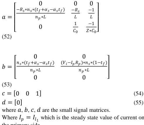
̂ is considered as input. The small signal matrices are given by,

𝑎 =

0

0

0

−𝑅𝑠∗𝑛𝑠∗(𝑡𝑓+𝛼𝑠−𝛼𝑠𝑡𝑓) 𝑛𝑝∗𝐿

−𝑅𝑠 𝐿

−1 𝐿

0

1

𝐶₀ −1 𝑍∗𝐶₀

(52)

𝑏 =

0

0

𝑛𝑠∗(𝑡𝑓+𝛼𝑠−𝛼𝑠𝑡𝑓) 𝑛_𝑝∗𝐿

(𝑉𝑖−𝐼𝑝𝑅𝑝)∗𝑛𝑠∗(1−𝑡𝑓) 𝑛_𝑝∗𝐿

0

0

(53)

𝑐 = 0 0 1

(54)

𝑑 = 0

(55)

where

𝑎

,

𝑏

,

𝑐

,

𝑑

are the small signal matrices.

Where

𝐼

𝑝

= 𝐼

𝑙1 which is the steady state value of current on the primary side.

The variation in duty cycle 𝛼̂ is considered in input matrix . Hence, the dimension of matrix 𝑏 is 2 ∗ 2.

B.Advantage of Proposed State Space Model of Full Bridge Converter

[image:5.595.302.548.388.602.2]

For obtaining the state space model of the non-isolated buck converter from the given result the terms 𝑁𝑝 and 𝑁𝑠

are neglected as they represent the turns of primary and secondary windings which are not present in the buck converter. The factors which consist of the resistance on primary and secondary side of the transformer are neglected. Hence the buck converter model can be obtained. The push-pull converter operates same as the full bridge converter the only difference between full bridge converter and the push-pull converter is that there are only two switches and the voltage is applied is half across the windings. The transformer windings are in four parts; two on the primary side and two on the secondary side. Hence, the factor of 2 is to be removed from the full bridge model.

V.CONCLUSION

The obtained state space model of the full bridge converter can also be used to determine the state space representation of other DC-DC converters. The obtained model can also be used to determine the ideal state space model which can help in design of converter for DC power supply based application. The state space model represents the full bridge converter in mathematical form which depicts the response of the system. Hence, from the response of the system the deficiency of the system can be identified and hence the compensator can be designed according to the deficiency of the primary system. As there is a variation in the proposed state space model from the ideal state space model, the compensator design varies. The compensator designed according to the proposed state space model has a significant improvement in case of high rating converters and hence the converter operation will be more efficient.

REFERENCES

1. L. Umanand, Switched Mode Power Conversion, NPTEL Lecture Series.

2. Katsuhiko Ogata, Modern Control Engineering, 5th edition, Pearson Education.

3. L.Umanand, Power Electronics: Essentials & Applications, Wiley Publications.

4. Robert Erickson, Dragan Maksimovic, Fundamentals of Power Electronics, Springer Science + Business Media, LLC.

AUTHORSPROFILE

Aniruddh Kulkarni is currently an undergraduate student pursuing Bachelors of Technology in Electrical Engineering at Institute of Technology, Nirma University, Ahmedabad, Gujarat. He has completed his secondary and higher secondary studies(HSC) from Vadodara, Gujarat.

P. N. Kapil completed Bachelors in

Engineering from Electrical Engineering

Department at Sankalchand Patel College of

Engineering, Visnagar under

Hemchandracharya North Gujarat University, Patan in May 2007 and subsequently pursued and completed Masters in Technology (M.Tech.) in Electrical Engineering with specialisation in Power Apparatus and Systems from Institute of Technology, Nirma University in May 2009. He has published 14 papers in various National / International Conferences and has published 01 paper as book chapter in a book published by Springer, India and has guided 22 M.Tech.