Simulation of the primate motor cortex and free arm movements in three dimensional space : a robotic arm system controlled by an artificial neural network

Retrospective Theses and Dissertations Iowa State University Capstones, Theses and Dissertations

1-1-1998

Simulation of the primate motor cortex and free

arm movements in three-dimensional space : a

robotic arm system controlled by an artificial neural

network

Lisa Marie Dauffenbach

Follow this and additional works at:https://lib.dr.iastate.edu/rtd Part of theEngineering Commons

This Thesis is brought to you for free and open access by the Iowa State University Capstones, Theses and Dissertations at Iowa State University Digital Repository. It has been accepted for inclusion in Retrospective Theses and Dissertations by an authorized administrator of Iowa State University Digital Repository. For more information, please [email protected].

Recommended Citation

Dauffenbach, Lisa Marie, "Simulation of the primate motor cortex and free arm movements in three-dimensional space : a robotic arm system controlled by an artificial neural network" (1998).Retrospective Theses and Dissertations. 17866.

movements in three-dimensional space: A robotic arm

system controlled by an artificial neural network

/

J

.:?

t

('

I

Lisa Marie Dauffenbach

A thesis submitted to the graduate faculty in partial fulfillment of the requirements for degree of

MASTER OF SCIENCE

Major: Biomedical Engineering Major Professor: Patrick

E.

Iowa State University Ames, Iowa

ii

Graduate College

Iowa State University

This is to certify that the Master's thesis of Lisa Marie Dauffenbach

has met the thesis requirements of Iowa State University

TABLE OF CONTENTS

CHAPTER 1. INTRODUCTION

Anatomy and Physiology of the Motor Cortex Motor Cortex and Control of Movement Motor Cortex in Behaving Monkeys Poisson Spike Trains

Simulated Actuator Purpose

CHAPTER 2. THREE-DIMENSIONAL REACHING: PRIMATE NEUROPHYSIOLOGICAL STUDIES

Materials and Methods

Animals and behavioral apparatus Training Neuronal recordings Data Analysis Epochs Regression model Population coding Weighting function

Neuronal population vectors

Rasters and peristimulus time histograms Cumulative sum technique

Sequential significant testing Results

Database

iv

CHAPTER 3. ARTIFICIAL NEURAL NETWORK MODEL

Background Model

Poisson process Input layer Hidden layer Weight matrices

CHAPTER4.ROBOTSYSTEM

PUMA Robot

Neural Network Connection

CHAPTER 5. SYSTEM PERFORMANCE

Final Remarks Future Research

REFERENCES CITED

32

32

35

35

42

44

47

47

52

54

58

CHAPTER 1. INTRODUCTION

Anatomy and Physiology of the Motor Cortex

The motor cortex was first identified by Gustav Fritsch and Eduard Hitzig in

1870 (Fritsch and Hitzig 1870) when a distinct area of the brain produced muscle

contraction on the contralateral side of the body from electrical stimulation

experiments in dogs. Soon after, David Ferrier (Ferrier 1875) provided strong

experimental evidence supporting Fritsch by stimulating a particular area of the

motor cortex that leads to movements of specific body regions.

It has been shown that the cortical surface of the monkey contains a motor

map of the body in an orderly, somatotopic pattern (Woolsey 1952). That is, the

distal hind limb is represented on the medial surface of the cortex and the proximal

hind limb is represented at the crown of the hemisphere, then the trunk, forelimb,

and face are represented progressively laterally. A similar motor map of the human

brain was also represented through neurosurgical procedures (Penfield and Baldrey

1937).

The motor cortex refers to cortical areas 4 and 6 in a region of the frontal

lobe. The primary motor cortex, also known as cortical area 4, is concerned with the

control of voluntary movement. It is an agranular type cortex, there is no granular

2

the primary motor cortex contains a population of Betz cells, giant pyramidal

neurons, whose large fibers terminate on spinal anterior gray matter and form

synapses on spinal interneurons (Shinoda, Yokota et al. 1981 ). Stimulation of

cortical area 6, anterior to the primary motor cortex, also produces motor effects and

is considered to be the premotor area. Axons project to the primary motor cortex,

subcortical structures, and to the spinal cord. The two principal premotor areas are

the supplementary motor area (SMA) and the premotor cortex.

Motor Cortex and Control of Movement

The brain communicates with the motor neurons of the spinal cord via axons

descending through the spinal cord along the lateral pathway and the ventromedial

pathway. The lateral pathway influences control of the distal musculature in the

extremities used in reaching and manipulation movements with the fingers and

hand. The ventromedial pathway influences motor neurons innervating axial and

proximal musculature that maintain balance and posture.

The lateral pathway consists of the corticospinal tract and the rubrospinal

tract. Approximately two thirds of the axons in the corticospinal tract originate in the

motor cortex, evenly dispersed between the primary motor cortex and premotor

areas. These axons leave the cortex and pass through the telencephalon and

thalamus via an internal capsule, through the midbrain and the pons, and collect at

pyramid-shaped bulge running down the ventral surface of the medulla. At the

junction of the medulla and the spinal cord, three-quarters of the corticospinal fibers

decussate across the mid line where the right motor cortex controls movement of the

left side of the body and the left motor cortex controls movement of the right side of

the body. Corticospinal axons influence motor activity directly on motor neurons and

interneurons and indirectly through the descending brain stem pathways. The

rubrospinal tract axons originates in the red nucleus of the midbrain and decussate

in the pons to join the corticospinal tract in the lateral column.

The ventromedial pathway tracts originate in the brainstem and terminate

among the spinal interneurons controlling proximal and axial muscles. The four

tracts consist of the vestibulospinal tract, functioning at the reflex control of balance

and posture of the head and neck, ensuring that the eyes are stable as the body

moves, the tectospinal tract, functioning at coordinating the head and eye

movements to an appropriate point in space, the pontine tract, facilitating extensors

of the upper and lower limb, and the medullary reticulospinal tracts controlling the

antigravity muscles of the limbs.

Motor Cortex in Behaving Monkeys

Edward Evarts was first to investigate the initiation or control of the motor

cortex in behaving monkeys. He recorded from individual pyramidal tract neurons in

4

simple task of wrist flexion and extension movements with varying extensor and

flexor loads (Evarts 1968). It was discovered that different populations of neurons

were active during flexion and during extension. Furthermore, the onset of their

activity occurred before the contraction of relevant muscles. Evarts then determined

that the firing rate of each neuron increased with load.

As the primary motor cortex influences multiple muscles, how the direction of

multijoint movement is encoded became of interest. Specifically, it was found that

motor cortical cells in behaving monkeys are broadly tuned with respect to the

direction of movement in two-dimensional (2-D) space (Georgopoulos, Kalaska et al.

1982) and later, to 30 space (Georgopoulos, Schwartz et al. 1986; Schwartz,

Kettner et al. 1988). A population of such neurons code accurately this direction.

Both the directional tuning and the population coding have been found to hold for

many motor structures (see Georgopoulos, Taira et al. 1993 for a review).

Together, they demonstrate that movement-related brain signals can be

successfully interpreted for the specification of a desired movement. It is noteworthy

that the amplitude of movement is coded additively in the discharge of motor cortical

cells, so that the directional tuning remains invariant for a range of movement

amplitudes (Fu, Suarez et al. 1993).

The variation of the activity of motor cortical cells related to proximal arm

reaching movements in the shoulder area of the motor cortex has been studied

(Georgopoulos, Kalaska et al. 1982; Georgopoulos, Kalaska et al. 1984; Schwartz,

intensity taking the form of a tuning curve represented by a cosine function. Uniform

representation of the sample population revealed that different cells fired in different

preferred directions such that many cells with different levels of activity throughout

the preferred direction spectrum were recruited into the active population. It was

then concluded that information about a particular movement could only be derived

from the entire active population (Georgopoulos, Kettner et al. 1988).

The main assumptions derived from these are collectively termed the

population vector hypothesis: (1) Each cell makes a contribution in its preferred

direction to the output of the entire ensemble; (2) The contribution strength is

determined by the cell activity in the direction of interest; (3) The vectorial

summation of all cells produce the ensemble output, known as the neuronal

population vector and points at or near the direction of movement. It can be said

that each cell "votes" in the direction of its preferred direction and the population

vector combines the votes into a weighted directional outcome. Each neuron

contributes only part of the information whereas the entire population determines the

direction of movement uniquely.

Poisson Spike Trains

It has been shown that actual motor cortical cell activity has similar firing

characteristics as a Poisson distribution. The Poisson spike train distribution,

6

modulation in relation to behavior. This analysis compares the number of spikes

that occur within a given time interval, the interspike interval (ISi), in an actual spike

train to the number of spikes predicted to occur in that time interval during a random

Poisson occurrence using the same mean discharge rate of the cell. In the actual

spike train, if the spikes occur non-randomly, the Poisson spike train analysis

determines significant changes in neuronal activity. The Poisson distribution serves

as a good null hypothesis because interspike intervals are distributed in an

approximately Poisson fashion (Rodieck, Kiang et al. 1962).

The similarities between Poisson generated spike trains compared with

actual spike trains recorded from a behaving monkey allows artificial simulation of

brain activity that is attained with a randomly selected Poisson distribution (Legendy

and Salcman 1985).

Simulated Actuator

The greatest potential from this research is in the design of prosthetic

devices. Understanding how cortical neurons work and what their activity describes,

it is possible to transmit the pattern of predictable activity in a language that makes

sense to an artificial arm and tell it to do what was initially intended. Researchers

began to implement this idea in the form of a computerized simulation (Lukashin,

Amirikian et al. 1996a). The central nervous system translates commands encoded

motor output that can be applied to the design of an adaptive system. This system

transforms neuronal activity from the motor cortex into a preferred motor output of a

multi-joint prosthetic limb.

Previous neurophysiological studies have shown that the population vector of

directionally tuned cells in the motor cortex can be used to predict future movements

in the arm. It was then conceived that the cortical neuronal signals could drive an

artificial actuator such that motor output would directly correspond to actual

performance. An extension of this study observed forces exerted by the arm

against an immovable object (Georgopoulos, Ashe et al. 1992). A model was

developed to simulate the mechanisms that produce an exertion of force based on

the neuronal signals that converge on the spinal cord (Lukashin, Amirikian et al.

1996a). Specific connection patterns between the populations of supraspinal

neurons and spinal cord interneurons were predicted such that the weights of the

network are based on the directional preferences of the interconnected units. The

idea was to train an artificial neural network such that reproducible experimental

data were achieved for stiffness characteristics of the human arm.

The experiment tested isometric force data in the presence of a constant bias

force over 8 directions in 2-D space (explained in Georgopoulos, Ashe et al. 1992).

A monkey was trained to grasp a handle with its hand pronated and exert a postural,

static force, P, that compensated the given bias force, B, and hold for a period of

time. A cue instructed an exertion of force, S, such that the force applied to the

8

dynamic force, I. Organization of the forces is explained by (Lukashin, Amirikian et

al. 1996a).

Impulse activity was recorded in the arm area of the motor cortex during 3

trials over 8 directions, hence 24 spike trains per cell. Directional tuning was

observed in approximately 56% of the cells recorded and was preserved across the

force biases. Cell activity varied with dynamic force but not with subject force.

Thus, the postural and incremental signals converge in the spinal cord and produce

an integrated signal to the motoneuronal pools (hypothesized in Georgopoulos,

Ashe et al. 1992).

Experimentally measured impulse activity from the motor cortex was used as

a time-varying input to the upper layer of a three-layered, feedforward, artificial

neural network. An intermediate layer, consisting of four model units, was

connected to a variable number of neurons in the upper layer, weighted with

corresponding strengths of synaptic connections. In accordance with the

connectivity between the upper and lower layers, the intermediate layer produces a

pattern of activity to six output units, in turn producing a time-varying pattern of

output activity that generates contractions of a simulated actuator muscle.

The three-layered artificial neural network obtains command signals from

actual neuronal activity obtained from recordings in the motor cortex of monkeys

performing the force task. Cell activity is recoded into motor actions of a simulated

actuator. The ANN is trained such that the synaptic connections between the three

al. 1996b). It was demonstrated that the generated force of summated neural

signals nearly equaled the summation of forces generated by each independent

signal. Moreover, it was shown that motor output was achieved with as few as 15

motor cortical cells. This important finding that a small ensemble of cortical cells

can reliably control complex motor output suggests that chronically recorded

command signals for artificially designed prostheses are feasible.

Purpose

Physiologically useful motor output requires multiple degrees of freedom

distributed over artificial limbs. The question of how motor cortical neurons

successfully move an artificial actuator has been addressed in computer simulation.

The time is ripe to apply this knowledge to the output of a robotic system that

corresponds to the performance of a real limb.

The research proposed consists of three components: (1) Simulate motor

cortical cell activity of behaving monkeys during a 30 behavioral task in the form of

a Poisson distribution; 2) Train a three layered feedforward artificial neural network

based on the directional preferences of the interconnected units; (3) Control a

robotic arm system off-line with the output generated by the ANN.

The spike activity of motor cortical cells in behaving monkeys performing a

30 task will be simulated as described in (Schwartz, Kettner et al. 1988) using a

10

neural network controller will receive the impulse activity of many cells fed as a

time-varying input to the upper layer of the network and transformed into an analog

command to be fed to the actuator. Each neuron at the intermediate layer will be

connected to all neurons at the upper layer. Intermediate neurons receive the input

signals as the sum of spikes from all upper neurons weighted with corresponding

strengths of synaptic connections. These inputs are accumulated over time and

transformed into activities of intermediate neurons using the sigmoid activation

function. At each instance of time, the collective activity of the intermediate layer will

produce a pattern of activity at the output layer in accordance with the connectivity

between these two layers. The output activity will then be transformed into analog

commands appropriate for the given actuator to produce off-line similar motor output

as that of the monkey. The feasibility of this approach has been documented in

studies using off-line neural recording and a modeled actuator (Lukashin, Amirikian

et al. 1996a). In summary, Poisson distributed cell activity will be used as real-time

CHAPTER 2. THREE-DIMENSIONAL REACHING:

PRIMATE NEUROPHYSIOLOGICAL STUDIES

Materials and Methods

Animals and behavioral apparatus

Two male rhesus monkeys (4-6 kg body weight) were used for this task and

described in detail in (Schwartz, Kettner et al. 1988). The animal sat in a small

Plexiglas chair secured inside a cubical enclosure. Movement was limited with Plexiglas waist and neck plates and a left arm restraint. This allowed controlled

movement with the animal's right arm. A 30 apparatus consisted of a cubical enclosure with a back metal plate that contained a 19 by 25 array of holes. Hollow

stainless steel rods, 45 cm-long, were threaded through the back plate for lateral

positioning located 15 cm away from the animal at shoulder level in the midsagittal

plane. These stimulus-response elements housed red buttons, 16 mm in diameter,

that illuminated from behind by a red light emitting diode (LED). Microswitches

detected depression with a force of approximately 200 g. The lights could be turned

on or off and dimmed in any combination as controlled by the computer program.

The center light was located directly in front of the monkey at right shoulder level

-- - - -- -- - - -- - -- ---.

12

Training

The animals were trained to reach with their right index finger from the center

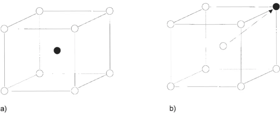
light to 1 of 8 peripheral lighted targets (Figure 2.1 ). The equal distances between

the center and targets allowed 30 sampling at equal angular intervals. There were

no restrictions imposed on movement trajectories, allowing the animal to see his

arm throughout the entire experiment.

~c

--

~-o

_{i f}

~0----_-

_

...

-·

/

~

-

__ ..

-/-

·

i

~/

/

•

_.0-

--

---

-

-

---0

o-·

---

~

0

---0

0---~

a) b)

Figure 2.1. The monkey was trained to reach for the center light (a) and then one of eight peripheral lights (b).

A trial started when the center light appeared. The animal was required to

reach for the center light and depress the switch for a variable period of time, the

control time (CT), until the center light then turned off and one of the peripheral

buttons became lighted. The time interval between the occurrence of the target

then moved to capture the peripheral light, the movement time (MT), and depress

the switch for another variable period of time, the target hold time (THT), after which

he received a liquid reward. An intertrial interval (ITI) of 2 sec intervened between

successive trials (Figure 2.2).

CL

CT

TL

RT

MT

n

Figure 2.2. A schematic outline of the behavioral task: CL (center light on,

-800 msec), CT (control time, -500 msec), TL (target light on, -1000 msec), RT (reaction time, -300 msec), MT (movement time, -500 msec), THT (target hold time, -200 msec), and TET (total experimental time, RT + MT).

The first step in training was to familiarize the animal with the apparatus such

that targets were captured as they were lighted. In the beginning, a juice reward

was given for merely touching the light as it was turned on. For all trials during the

training period, the light appeared first in the center and then in one of 8 targets.

This task of moving in directions away from the common starting position is called

14

animal learned to move from the center light to the peripheral light, the conditions of

juice reward timing changed such that holding the center light was not sufficient,

rather for moving towards the peripheral light and holding it for a period of time.

Initially, the CT was short, but as training became more defined, the time increased.

Similarly, the THT was also increased.

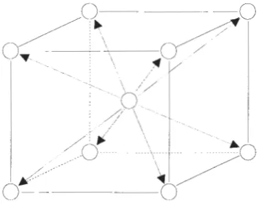
Figure 2.3. Center-> out task.

Prior to beginning a trial, all variables were set. The minimum CT was set to

0.5 sec and the minimum THT was set to 0.15 sec to receive a liquid reward. An

upper limit of 1 sec was set for both the reaction and movement times. In

subsequent trials, different targets were lit such that all 8 targets were presented in

a random sequence, or randomized block design. Each training session consisted

Neuronal recordings

Neuronal activity of single cells in the motor cortex were recorded

extracellularly during the 30 task using standard cell recording techniques

(Schwartz, Kettner et al. 1988). Recently, a seven microelectrode matrix recording

system (U Thomas Recording, Germany) (Adapted by Mountcastle, Reitboeck et al.

1991) and described in detail in (Reitboeck 1983) and (Reitboeck 1983)) was used

to record extracellular activity (Georgopoulos and colleagues, unpublished data) .

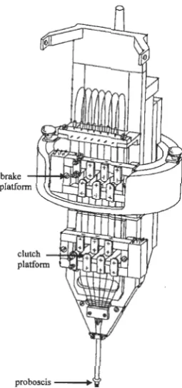
This assembly (Figure 2.4) consisted of a moveable clutch platform that drove the

microelectrodes in 2 µm steps by a stepping motor and a stationary brake platform

that held them firmly in place. Seven multi-segmented electrode guide tubes were

aligned between the movable clutch and the stationary brake. Manipulation of

individual electrode depth occurred through the microdrive's independent control of

both platforms such that any electrode may be fixed to the movable platform and

freed from the fixed platform in a clutch-brake action. This allowed several

electrodes to be arranged in a choice of spatial patterns. As they were driven out of

the matrix, electrode spacing was managed by the various configurations of the

proboscis (see Figure 2.4). The direction, forward or backward, and movement

speeds were operator controlled.

The microelectrodes (U Thomas Recording, Germany) were made of flexible

quartz fibers with a platinum/tungsten core having an outer diameter of 80 µm and a

core diameter of 15 to 30 µm. A high-temperature electrode tip puller (Modell EL-1,

16

desired slope and size. They were ground mechanically with a precision diamond

grinding disk (Tip Grinding Maschine, Model DI-LU, U Thomas Recording) to a

tapered tip of -14 µm, and an impedence of -2 Mn. The quartz glass fiber

electrodes were stiff enough to transit the dura without breaking, yet fine enough to

produce action potential amplitudes unaffected by behavioral movements. Minimal

neuronal damage occurred due to electrode flexibility and smoothness (Mountcastle,

Reitboeck et al. 1991 ).

proboscis

A recording chamber with an internal diameter of 18 mm was stabilized to the

animal's head over the arm area of the motor cortex. The chamber was fluid-filled

and hydraulically sealed. The cranial cavity was cleaned of bone, filled with

gentamicin sulfate and closed with a sterile acrylic cap. A metal halo was positioned

on the skull to immobilize the head during the experiment and secured with dental

acrylic to cement the devices to small anchoring screws inserted into the skull.

On the day of recording, the animal's head was immobilized to the primate

chair and the mechanical microdrive was attached to the recording chamber. The

proboscis of the matrix was lowered directly above the dura. Positioning of the

microdrive allowed microelectrode penetration within a 14 mm diameter circle and

forward motion control to the 1-µm level. Advancement of the microelectrodes into

the cortex occurred one at a time, until signs of neural activity were encountered.

The electrical signals of single neurons in the motor cortex were recorded

extracellularly. Action potentials were identified (Mountcastle, Talbot et al. 1969),

amplified and displayed on oscilloscopes. Differential amplitude discriminators

separated the action potentials based on the amplitude of the potential. Initially

negative-going potentials were selected, indicating an undamaged neuron, however

upon entry into the white matter of the cortex, the negative-going potentials turned

to purely positive spikes. Some penetrations were made in which to pass current at

the electrode tip for marking purposes (3-4 µA for 3 sec). Once a neuron was

isolated, only arm-related cells were selected for further study. This eliminated

18

The neuronal population consisted of 475 directionally tuned cells out of 568

isolated cells (Schwartz, Kettner et al. 1988).

Data Analysis

Epochs

The data were evaluated according to standard statistical techniques

(Snedecor and Cochran 1989 and Draper, 1981 #13) and display techniques

(rasters, histograms, etc .... ). Four epochs were calculated for each trial: (1) the

control time (CT), the period in which the center light was pressed by the animal

until the peripheral light turned on; (2) the reaction time (RT), the period from the

appearance of target stimulus to the onset of movement; (3) the movement time

(MT), the period of movement from the center light to the peripheral light; and (4) the

target hold time (THT), the period in which the target light was pressed to receive a

liquid reward. The total experimental time (TET) is the combined RT and MT

epochs (see Figure 2.2). An analysis of variance (ANOVA) was performed to test

the differences in mean cell activity for each direction of movement.

Regression model

Multiple linear regression (Draper and Smith 1981) was used to further

analyze the cell activity. This related the cell discharge rate to motor parameters,

system, XYZ positive axes, with origin at the center light was used. A vector, M,

represented the movement direction in 30 space with unit length. This vector uses

angles,

x.

My =cos \Jf, (2.1)

and

~M

₌

x y z (2.2)

It has been determined previously (Schwartz, Kettner et al. 1988) that the cell

activity in relation to the direction of movement may be quantified in the following

equation:

(2.3)

The rate of cell activity is d(M) and bx, by, bz are cell varying coefficients determined

by multiple linear regression techniques. The direction of movement, vector C,

where the cell activity is highest is known as the cell's preferred direction. The

and

20

bz

C=-

Equations (2.4) are substituted into the rate of cell activity equation, (2.3):

A dot product relationship is used for vectors, C and M:

where /C/ and

IMI

M,

e

formed between the preferred direction, C, and the direction of movement, M.

Equation (2.6) is rewritten:

(2.4)

(2.5)

(2.6)

Also,

d(M)

=

=

=

/

Ci= !Mi= 1

since vectors C and M are of unit length and are substituted into equation (2.8): (2.8)

(2.9)

d(M)

=

Equation (2.10) has been referred to as the directional tuning function (Schwartz,

Kettner et al. 1988). This function implies that the rate of cell activity will be highest

when the movement in 30 space is in the cell's preferred direction. This

coincidence of movement occurs when vectors C and M correspond. The rate of

cell activity allows only values greater than or equal to zero. Thus, in the case of a

negative value, the rate is set to zero.

A randomized block design was used and discharge rates were averaged

over the 5 - 8 repetitions. The variability of the preferred direction among the

22

s·

=

_

(n_-R_)

n

'

o

s

s

·

s

The number of directions, one for each repetition, is n and the length of the resultant

is R. A spherical variance value near 1 indicates that the preferred directions

among the repetitions have a high variability, whereas a value near O indicates low

variability.

An index of directional modulation was used to normalize the depth of

directional tuning among the peak-to-peak sinusoidal preferred directions:

(b

0)

Population coding

It is assumed that the i1h neuron makes a vectorial contribution in a preferred

direction, Ci, with a magnitude of wi(M). Also, the contributions taken from all eight

movements sum to yield a neuronal population vector:

N

P(M) =

L

(M)c

i=1

where N is the number of neurons in the population vector summation and wi(M) is

selectivity of single cells, weighs vectorial contributions on the basis of change in

cell activity and produces a unique output. Once the population vector is

determined, it can be compared to the movement vector for congruence. Further

analysis of equation (2.13) included a spherical correlation, p, between the

population vector and the movement vector and the angle between them.

Weighting function

The i1h cell in a population vector has a preferred direction, C, that is the same

for different movements. The magnitude of the vector, wi(M), is based on the

discharge rate of the neuron, D~, during the movement vector, M. Consider that n

is equal to the number of repetitions of movement in each of the 8 directions and

that d'i(Mi,k) is the discharge rate of the i1h neuron during a TET, total experimental

time, epoch of the k1h repetition in the j1_{h direction. In one movement direction, the}

discharge rate is observed as the summation over all repetitions:

Observation is done for all movement directions:

_ , 1 8 '

Dij =-L.Dr

n j=1 ~

(2.14)

24

Using the directional tuning function in equation (2.10), the discharge rate can be

rewritten:

(2.16)

wheree cM is the angle between the cell's preferred direction vector and movement

vector. Various weighting functions were tested. In essence, the movement

direction is regarded as the weighted sum of vectorial contributions such that each

neuron "votes" in its preferred direction. The vote is weighted according to the

change in cell activity during a particular movement and the population vector points

towards the direction of reaching.

Neuronal population vectors

The direction of movement represented by a population of cells has a unique

orientation such that it is broadly tuned. Essentially, cell activity is most profound for

a movement in a particular direction and decreases progressively for movements

farther away from the preferred direction. Each vector represents a contribution of a

single neuron in its preferred direction and its length is associated with the change

in activity according to the actual direction of movement. The neuronal population

vector is the weighted vector sum consisting of only directionally tuned cells and

conveys a directional signal with as few as 100 to 150 cells (Schwartz, Kettner et al.

including motion from different origins (Caminiti, Johnson et al. 1991 and Kettner,

1988 #16), and isometric force pulses (Georgopoulos, Ashe et al. 1992).

Rasters and peristimulus time histograms

Graphical representation of single-cell activity is displayed in the form of a

raster. The spike train for each trial is aligned to the time of a behavioral event,

such as the presentation of a stimulus or onset of movement. Each row of activity

(y-axis) represents a trial and each spike represents an action potential over time

(x-axis). If there is no or little spike train activity, the raster will appear blank and the

cell is excluded from data analysis. The raster is divided into bins (pre-determined

sets of time) that are averaged and normalized to create a qualitative assessment of

the neural activity in the form of a peristimulus time histogram.

Peristimulus time histograms (PSTHs) are used extensively in

neurophysiology to investigate the behavior of neurons from the available

extracellularly recorded action potentials. As the action potentials discharge a

number of impulses, in the form of a raster, a histogram is formed from the sum of

all trials. Spike trials were summed using a pre-determined bin length of 20 msec.

The mean value of activity was determined by dividing the number of spikes by the

number of trials. Time was normalized by multiplying the mean value by the number

of bin lengths in one second (for example, a 20 msec bin length would give 50 bins).

Thus, the histogram height is a function of spike rate and the length is determined

--~ --- - - -

-26

Cumulative sum technique

The cumulative sum technique (CUSUM) (Ellaway 1978) is a simple

statistical method that analyzes peristimulus time histograms by detecting changes

in single-cell activity. This technique has the advantage of smoothing the activity of

the data without distorting the original data as well as providing an immediate visual

impact. Change is detected by changes in the value of the slope, which is the

difference between the mean level of a particular period of time and that of the

reference level. In this experiment, these changes were observed 500 msec before

the onset of the target light.

A peristimulus time histogram was first constructed for each of the 8

directions of movement. The standard deviation, cr, was calculated for the 25

control bins (500 msec I 20 msec bin length) to test the significance of spike rate

over time. The CUSUM technique takes the difference between the mean control

rate of the 25 control bins and successive bin rates, or reference level, starting at

the time of target onset. A new series of points were formed by adding up the

differences consecutively and plotting on a cumulative sum chart. When the

reference level rates do not differ from the control rates such that they are equally

effective, the CUSUM value is zero. This is known as a null hypothesis.

Fluctuations occur by chance above and below zero producing a probability of

change, a1 and a2 (Armitage 1975). It is customary to add the two probabilities for a

two-sided test at the 2a significance level. To specify the sensitivity, it is important

probability of type II error. Thus, it is necessary to test the statistical significance of

a particular deviation using a sequential significance test.

Sequential significant testing

Upon visualizing a change in slope on a cumulative sum plot, it is necessary

to question the significance of the change. There is a higher probability of finding a

significant difference purely by chance when the test of significance is performed

repeatedly (Armitage 1975).

In this experiment, upper (positive) and lower (negative) boundaries were

established to determine a significant increase or decrease, respectively, of the data

set. There are three factors contributing to the calculation of the boundaries: (1) It

was assumed that the variability of the differences between the mean control rates

and the successive bin rates were not different from control period observations,

thus the standard deviation, cr, was used. (2) The pre-determined boundaries that

segregate significance expand as the bin number increases as a result of repeated

performances of significant testing. (3) The statistical plan involved was closed and

restricted in effect of the repeated testing for a regulated amount of time. A

two-sided level of significance was desired. Equations for the upper and lower

boundaries were determined (Armitage 1975, p. 97):

U: y

=

L: y

=

(2.17)

28

where cr is the standard deviation as described and n is the bin number that is

incremented with onset of the target light. The constants, a and b, relate to a

closed, restricted plan and were determined from (Armitage 1975 Table 5.3, p. 101 ).

Given that 2a = 0.033, 1-P = 0.95 (power), 81 = 0.7 (indicating the magnitude of

difference between probabilities that are detected with high power) and the

maximum number of testing (N) = 36, it is determined that a = 5.2 and b = 0.35.

The pre-determined bin length was 20 msec and the average THT was 730 msec,

thus N

=

equations for the upper and lower boundaries are:

U: y

=

+

L: y

=

(2.19)

(2.20)

To stop the trial, strong evidence must be displayed for statistical difference.

Thus, one of the following events must occur: (1) On the cumulative sum plot, either

boundary was crossed by a CUSUM value. To measure the consistency of change,

two of the resultant bins must also produce a significant change in the same

direction. (2) The animal released the target light and the trial ended before change

occurred. (3) N = 36 consecutive tests were performed and the CUSUM value did

not cross either boundary. It may be possible that a change will occur in

A cumulative sum plot using the sequential significance technique is

described in (Schwartz, Kettner et al. 1988). Movements in two different directions

in 30 space are plotted using spike trains from 8 repetitions. The CUSUM crossed

either boundary on the 7th bin (20 msec x 7 bins

=

activity). To stop the test, 2 subsequent bins must also show a significant change in

the same direction, therefore a change in activity was detected 140 msec after the

onset of the target light.

Results

Database

In order to determine significant variation of cell discharge with respect to the

direction of movement, an ANOVA was performed. Next, multiple linear correlated

the discharge rate described by the tuning function. Three types of cells were

encountered. Four hundred seventy-five (83.6%, TET epoch) cells were shown to

possess significant changes in activity with respect to movement direction with a

good fit of the directional tuning function and were considered directionally tuned.

Thirty-one (5.5%, TET epoch) cells were shown to present significant changes in

activity with respect to direction but did not fit the directional tuning function and

were considered irregular. Finally, 62 (10.9%, TET epoch) cells were shown to

exhibit activity during the task though did not significantly differ among the task

30

Neuronal population coding

It follows from the directional tuning function (equation 2.10) that motor

cortical cells are active with movements in many directions and that a movement in

a specific direction recruits many neurons. Thus, the entire active population is

involved in the generation of reaching movements. It can be assumed that each

neuron represents a vector; each vector represents the directional influence along

the axis of the neuron's preferred direction. The length of each vector is

proportional to the change in the neuron's discharge rate from a particular point.

Representation from all neuronal vectors in the active population come

together as a neuronal ensemble such that the combine directional outcome is in

the form of a population vector, the weighted vector sum of individual neurons. It

can be said that each cell "votes" in the direction of its preferred direction and the

population vector combines the votes into a weighted directional outcome. Each

neuron in the population vector contributes only part of the information, whereas the

entire neuronal population determines the direction of reaching uniquely. The

population vector does not depend exclusively on a particular cell and can be

calculated from smaller samples of cells randomly selected from the original

ensemble. Thus, a population size of 150 to 200 cells sufficiently estimates the

direction of the population vector within 10 to 15 degrees (Georgopoulos, Kettner et

al. 1988). The direction of the population vector is very close to the direction of

movement vector (Georgopoulos, Schwartz et al. 1986, fig.4) and is therefore an

Planned movement

The information represented by the population vector is assumed to be about

direction. The involvement of the motor cortex under various behavioral conditions

was documented such that the population vector was calculated every 10 or 20

msec during the reaction time (Georgopoulos, Kettner et al. 1988), delay periods

(Georgopoulos, Crutcher et al. 1989) and memorized delay periods (Smyrnis, Taira

et al. 1992). In the presence or absence of immediate motor output, the directional

information was kept in memory and the representation of intended movement was

displayed in the form of a population vector. Essentially, the vector pointed in the

direction of planned movement.

In the 30 reaching task, approximately 300 msec intervened between the

onset of the target stimuli and movement. The cell activity in the motor cortex

precedes the onset of movement on the average by 160-180 msec (Georgopoulos,

Kalaska et al. 1982), but does it predict the direction of the upcoming movement

during the reaction time? It was shown that the population vector does indeed point

in the direction of movement 160 msec before the onset of movement

32

CHAPTER 3. ARTIFICIAL NEURAL NETWORK MODEL

Background

Computational paradigms that implement simplified models from their

biological counterparts are considered to be artificial neural networks (ANNs). They

represent the massive interconnections between simple neurons which are typically

modeled by a sigmoid function. The abstraction of the nervous system architecture

forms the basis behind ANNs in that computing units are joined together by

connections, modeled from neurons and their synapses, respectively. Dynamic

network models provide useful tools for simulating neural mechanisms that generate

patterns of activity in motor systems (Fetz and Shupe 1990).

There are several advantages for using neural network models. The most

attractive feature is their ability to learn and perform computation based on similarity.

This ability comes forth through straightforward synaptic connections modified

accordingly. As computational systems, they exhibit graceful degradation known as

a toleration to imperfect input or corruption of the internal performance. An

important property of networks is pattern completion, whereby taking an incomplete

input pattern, sufficiently similar to trained inputs and lead to a behavior extracted

the input pattern is linked with the "correct" output through a set of connections with appropriate weights (Barnden 1994 ).

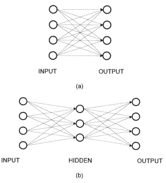
The need to control complex systems has led to new methods for developing neural network models. In the most common feedforward neural network, there may be a single set of modifiable connections in between the input and output layers or multiple layers of connections (Figure 3.1). In this paper, ANNs having a three-layered, feedforward architecture will be considered.

INPUT OUTPUT (a)

INPUT HIDDEN OUTPUT

(b)

Figure 3.1. Feedforward artificial neural network without hidden layers (a)

34

To make associations between the input and output patterns, a set of

connections that link the two patterns form a matrix of connection weights. In

general, ANNs have a training rule such that connection weights are adjusted on the

basis of data to improve performance. They learn from examples and are capable

of generalizations beyond the training set. Weight values are usually assigned from

a fixed, off-line algorithm or adjusted during the learning process. This learning

process adjusts the weights step by step and stores the best values as the final

connection strengths.

The ANN allows never before presented examples of data to be correctly

recognized based on a standard learning protocol. The trained network generalizes

information from a restricted number of teaching examples, the training set, and

uses it to identify new examples of the same data (Amirikian and Nishimura 1994 ).

Having learned associations from the training set, the network has the ability to

generate a correct output to a new set of input patterns.

The initial training set of input patterns have a known set of desired output

patterns. An input pattern from the training set is selected and given to the network

to generate an actual output. Comparison of the desired output pattern to the actual

output pattern produces an error signal, whereby weight connections are adjusted to

Model

A general description of the paradigm is graphically represented in Figure

3.1. Essentially, spike train data is simulated with a Poisson process from actual

data recorded from behaving monkeys performing a 30 reaching task in each of

eight directions around a cube. The spike trains are fed into the upper layer of the

ANN at each bin length to produce three output units corresponding to x, y, and z

coordinates as robot end-points that directly correspond to the original movement

trajectory.

Poisson process

The basic elements of the network are neurons with similar firing

characteristics as compared to single motor cortical neurons during 30 reaching in

behaving monkeys. It has been determined that the time series of spikes fired by a

single cortical neuron could be well approximated by a Poisson process (Rodieck,

Kiang et al. 1962). In the framework of this approximation, the probability of n

spikes occurring in the time interval Tis given by:

36

where a is the firing rate (number of spikes fired during a unit time). The probability

density distribution of interspike intervals is given by:

where t1 is a time interval between two adjacent spikes. The Poisson process is

simulated by generating consecutive ISls according to the following expression:

-1

t1 = -log(1-RND)

a

where RND is a randomly generated number between 0 and 1.

(3.2)

(3.3)

A histogram of the generated IS ls compared to P(t1) is shown in Figure 3.2.

As the total time T increases, distribution of ISls obtained from the generated spike

train approaches the true Poisson distribution. The purpose for this comparison is to

test that the generated spike trains indeed have the Poisson distribution. A

distinctive feature of the Poisson distribution is that the mean of t1 is equal to its

standard deviation.

The movement vectors correspond to the eight movements of the monkey

performing the 30 reaching task as described by (Schwartz, Kettner et al. 1988).

The coordinates of the cube ranging from -1 to 1 in all dimensions (Figure 3.3) and

>.

:!::::

:0 co

..c

0

....

a..

0.4

0.35

0.3 -·

-0.25 _--P(t)

•

0.2 _{- -• - -Generated Poisson (100 sec)}

0.15

0.1

0.05

0

0 0.05 0.1 0.15 0.2 0.25 0.3

Bin Length (sec)

Figure 3.2. Comparison of generated Poisson spike trains to the Poisson probability distribution at T=1 sec and T=100 sec.

(J.)

M1

=

M2

=

M3

=

M4

=

M5

=

Ms

=

M7

=

Ma

=

..

~ a N

...

(-1,-1, 1)

(-1,-1,-1)

(-1, 1,-1)

(1,1,1)

(1,-1,1)

( 1,-1,-1)

(1,1,-1)

38

0

Y-Axis

Preferred directions of the input neurons are uniformly distributed in 30 space

according to the probability density distribution:

1 .

F( 8,cp)

=

where angles 8 and cp determine the location of the unit vector in 30 space (Figure

3.4).

Each input neuron was assigned a preferred direction vector given by the

following pair of angles:

8

=

_(3.5)

and

cp

=

₍₃

_.

₆₎

Equations

(3.5

3

.

6)

uniformly in 30 space.

Let \J' be the angle between the movement vector M and the preferred

40

z

e

y

x

where {Mx, My, Mz} and {PDx, PDY, PDz} are x, y, and z components of the

vectors Mand PD, respectively. The transformation from polar to Cartesian

coordinates is given by:

PDx =sine coscp

PDY =sine sincp

(3.7)

(3.8)

(3.9)

PDx =case (3.10)

The units at the input layer receive signals from motor cortical neurons.

Neurophysiological studies demonstrated that their activity is directionally tuned

(Georgopoulos, Schwartz et al. 1986; Schwartz, Kettner et al. 1988). Namely, there

is a simple relationship between the mean firing rate of the cell and the angle \J'

between its preferred and movement directions:

42

where band k are defined by the maximum, Amax, and minimum, Amin, firing rates of the cell:

Amax +Amin

b=- -

-2

Amax -Amin

k= - -

-2

(3.12)

(3.13)

Note that the cell fires at its maximum rate when movement is made in its preferred direction (\J' = 0°) and it fires at its minimum rate when the movement is

made opposite to its preferred direction (\J' = 180°).

Input layer

The network receives generated Poisson spike trains as a time varying input

and transforms them into a time-varying output. Each input unit receives a spike

train corresponding to one neuron. An input unit accumulates spikes over time in

are accumulated and given a number, the number of spikes in that bin. All spikes in

the second bin, 20 msec to 40 msec, are accumulated and given a number added to

the number in the previous bin. This calculation continues until the end of the spike

train is reached. The hidden layer receives information, one bin at a time, starting

with the first bin.

Hidden layer

The hidden layer units are assigned preferred directions which are uniformly

distributed in 30 space with angular deviations nearly equally spaced from one

vector to another. To fulfill this requirement, the following procedure was adopted.

A value of parameter k was fixed which could be any non-negative whole number (0,

1, 2 ... ). The number of vectors generated monotonically increased the function of k.

Second, a set of angles

e

i

i

=

For each

e

i

44

where

The operator

L-J

unit vectors generated by this procedure is equal to:

(3.16)

Equation (3.16) adds two additional vectors that point to the north and south

poles of the unit sphere in Figure 3.4. The polar coordinates of each preferred

direction vector are converted to Cartesian coordinates using the standard

transformation equations (3.8 - 3.10).

The number of cells at the hidden layer is equal to N101• In routine simulations,

k

=

=

Weight matrices

The weight matrices are calculated according to the preferred direction

vectors at the connection units. In the case of the three layered feedforward ANN,

hidden layers and the other connection between the hidden and output layers. In general, the strength of connection from neuron j to neuron

i

following equation:

(3.17)

where \f'ii is the angle between the preferred direction vectors of connected units, a

is a variable used for adjustment of the performance of the model, and Nin is the

number of input units. The connections between the input and hidden layer were

assigned in the following manner. The preferred directions of the hidden units have been determined according to the procedure described in the previous section using

equations (3.14 - 3.16). The preferred direction of the input units were drawn from

random uniform distribution as described in equations (3.5 - 3.7).

The cosine of the angle \f'ii between preferred direction vectors of unit i at the

hidden layer and unitj at the input layer is given by a dot product of the vectors:

(3.18)

where {

lj,

I~,

lj}

H~,

Hi,

H~}

direction vector corresponding to the input and hidden units, respectively. The

46

W!i

=:.

(1jHf +

l~Hr

+ l}Hn

m

(3.19)

The weight matrix describing connections between the hidden and output layers was defined in a similar way. The output layer contains three units, x, y and z

which specify end-point positions of the robot arm in a Cartesian coordinate system.

The preferred direction vectors assigned to the three output units simply correspond

to unit vectors in the positive direction of the x, y and z axes.

01 = (1, 0 ,0)

02

=

03 = (0, 0, 1)

The connections between the hidden and output layers are then given by:

W!i

=:.

(ojHf

+O}Hn

(3.20)

where {

Oj,

Oj}

CHAPTER 4. ROBOTIC SYSTEM

PUMA Robot

The Unimate PUMA Mark II, 200 Series Robot is a computer controlled robot

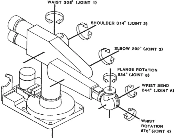
arm system manufactured by Unimation Incorporated of Danbury, Connecticut. Six

degrees of freedom provide flexibility and design to adapt to a wide range of

applications. Each member of the robot arm rotates around one or more axes and

is connected to another member at a joint, similar to a human arm. The members

include the trunk, shoulder, upper arm, lower arm, wrist, and gripper (Figure 4.1).

WAIST 308° (JOINT 1)

WRIST BEND 244° (JOINT 5)

WRIST ROTATION 578° (JOINT 4)

48

An initializing procedure must be performed each time the system is powered

up preparatory to running. Position is measured relative to an absolute position, the

nest position. After performing this calibration procedure, the PUMA system is

ready for teaching or running a software program.

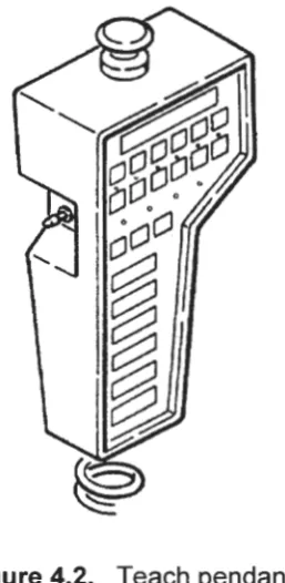
The basic units of the PUMA system include a teach pendant, software,

controller, peripherals, and the robot arm. Positioning of the robot may occur by

manipulating the joints via the microprocessor based teach pendant (Figure 4.2).

Figure 4.2. Teach pendant.

Several teach modes provide flexibility and control via an LED display. The

Comp mode allows the control to switch back to the computer. The Tool mode

preconditions the X, Y, and Z pushbuttons to move the robot along the tool

coordinate system, defined by the tool transformation (for example, pressing one

linear motion of the tool along its own axis). Whereas, the World mode

preconditions the X, Y, and Z pushbuttons to move along the world coordinate

system, fixed to the base of the arm. The Joint mode preconditions motion to move

a single joint in either a positive or negative direction. Only one motion may be

driven at one time. Finally, the Free mode allows direct manual movement of the

arm. The appropriate joint is selected to be released and is positioned by the

operator in any desired configuration.

The PUMA system comes equipped with a personal programming language

developed for assembly. Programming is accomplished with the teach pendant or

by keyboard entry. Points that are taught to the robot are stored as transformations

and referenced to a coordinate system fixed relative to the stationary robot base.

The controller is the main component of the PUMA system (Figure 4.3). All

signals to and from the robot pass through the controller and perform real-time

calculations to control arm movement and position. Each joint of the PUMA arm is

driven by a permanent magnet servomotor through a gear train, a motor that drives

movement around a joint. A servomotor is a DC permanent magnet motor that

reacts quickly and smoothly to changing drive level inputs. One is used to drive

each joint on the robot. Servomotors incorporate incremental encoders that send

information about arm position and velocity to the controller providing feedback for a

50

Unimation Inc.

ELAPSED TIME

c I I I I I J AUTO START

0

AR"' POWER OH

POWER ON _HALT

®

UNIMATE

~

COMPUTER/CONTROLLER

0

0

MANUAL CONTROL

Figure 4.3. Controller.

The peripheral components receive information. A terminal contains a video

unit and keyboard to communicate with the controller by teaching or editing software

programs.

There are two procedures that may be used to teach the robot. The teach

pendant manually directs the movements of the robot arm through each step of the

task while the coordinates are recorded and stored in computer memory. The

second method is to write a software program that incorporates position data into

memory through the peripheral terminal keyboard or through the teach pendant. In

Neural Network Connection

An interface from the ANN to the assembly language of the PUMA robot was

created to send the output generated by the ANN. At each time bin, three output

units yield the Cartesian x, y, and z components of the robot's end-point position.

This information, encoded in nine bytes, is transmitted to the robot. Each coordinate

of the vector is given three bytes per axes for a total of nine bytes through the serial

port. The assembly language routine stores the information in buffer memory until it

is accessed by the robot. A program was written in the assembly language to read

the buffer memory and send the coordinates to the robot via the controller. Scaling

of the robotic coordinate system was necessary to create movement of the robot

arm, of desired amplitude and speed was adjusted to achieve trajectories similar to

52

CHAPTER 5. SYSTEM PERFORMANCE

The actual trajectory generated by the network was compared to a desired

trajectory to determine the performance of the system. The performance was

assessed as a robot-mean-square error between the desired and actual trajectories

for all eight movement directions:

(5.1)

where the radius vectors

R1(tj)

Rf (t

j

)

between the desired trajectory

i

time bin

tj

Nr

The trajectory error was averaged over 100 trials and represented in Figure

5.1 as a function of the number of cells at the input layer. Direction and amplitude of

the error signal was normalized to 1. It is seen that 100 to 150 cells are sufficient to

reliably generate desired trajectories and is consistent with previous findings

54

A three-dimensional view of the generated and desired trajectories are

displayed in Figures 5.2 - 5.4. As the number of input neurons increases, the

generated trajectories more closely resemble the desired trajectories.

Final Remarks

The purpose of this experiment will be evaluated in light of the results of this

investigation.

To simulate motor cortical cell activity of behaving monkeys during

a

behavioral task in the form of a Poisson distribution. Motor cortical cell activity from

behaving monkeys performing a 30 task was simulated according to the Poisson

distribution function and randomly generated interspike intervals were similar to

actual data. Accumulated interspike intervals created a simulated spike train that

was used as one input neuron into the upper layer of an artificial neural network.

To train

a

directional preferences of the interconnected units. A three layered artificial neural

network with 150 input unit neurons, 6 hidden layer units and 3 output units was

created to use the simulated spike train data for each input neuron and generate a

Cartesian coordinate as output. Weighted connections between each layer were

assigned from a fixed, off-line algorithm based on directional preferences of the

interconnected units. The generated output trajectories of the artificial neural

en

~

I N

~ I

-1

\',

0

Y-Axis

~

..

1

0

X·Ms

Figure 5.2. Example trajectories generated by 50 input neurons.

Actual Trajectory

Desired Trajectory

T"'"

"'

~

a

N

T"'"

I

-1

0

1

Y-Axis

Figure 5.3. Example trajectories generated by 100 input neurons.

Actual Trajectory

Desired Trajectory

01

C/J

~

I

N

"t""

I

·1

0

1

Y·Axis

Figure 5.4. Example trajectories generated by 150 input neurons.

Actual Trajectory

Desired Trajectory

58

as the number of input unit neurons increased. Approximately 100 - 150 input

neurons were sufficient to produce an actual trajectory similar to the desired

trajectory.

To control a robotic arm system off-line with the output generated by the

ANN. A robotic arm system with six degrees of freedom was used to visually

represent the actual trajectories generated by the artificial neural network.

Cartesian coordinates were sent through a serial port to the assembly language of

the robotic arm system and stored in buffer memory. The workspace of the robotic

arm was scaled and speed was adjusted to create movement of similar to an actual

arm. Successfully, the robotic arm system accessed the Cartesian coordinates in

buffer memory through its own assembly language and moved in the actual

trajectories created by the artificial neural network.

Future Research

Time constraints prevented further training of the ANN in order to decrease

the trajectory error. The next step in this project is to utilize the hidden layer such

that actual trajectories more closely resemble desired trajectories.

It has been demonstrated that Poisson spike trains that model spiking activity

of directionally tuned motor cortical cells with preferred directions randomly