Asymmetric Volatility Modeling and Leverage Effect of Nifty Stocks

Asymmetric Volatility Modeling and Leverage

Effect of Nifty Stocks

Jincy K John, R. Amudha

Abstract: This research article investigates the heteroskedastic behaviour of the NSE Nifty stocks representing the Indian equity market. It attempts to explore the effects of both bad or good news on volatility experienced in the Indian stock market during the period from 2003 to 2017 (The period when market has experienced both bull and bear phases). The price behaviour of auto sector stocks from NSE was used to predict the volatility. The standard GARCH models were applied to study whether there is volatility during the period of study and two commonly used asymmetric volatility models i.e EGARCH and TGARCH were employed to assess the leverage effect. The study reports an evidence of volatility which exhibits the clustering and persistence. The return series of the stocks selected for the study are found that they react to the bad news and good news asymmetrically. The research concludes that the negative shocks to these stocks deliver more volatility than the positive shocks, of the same magnitude.

Key words: Volatility, Leverage effect, GARCH models. JEL classification:C13, C52, C53, C58, G10, G17.

I. INTRODUCTION

The important attribute of any financial instrument is stochastic nature of its returns and this spread of outcome is the volatility. It is a phenomenon which characterizes changeableness of a variable under consideration. Volatility is allied with unpredictability and uncertainty of stock movement, which is one of the key parameters influencing the numerous financial decisions. Financial markets play a key role in shaping the economic conditions of any nation. In the recent past, there is a growing importance for estimating and analyzing volatility and extensive research has been done on the modeling of financial time series. Estimation of volatility addresses the issues in the risk management and helps to manage portfolio efficiently. Reliable volatility estimation is crucial for hedging against risk and portfolio management. And several studies have shown the modeling of the stock market volatility of developed and developing countries. Many researchers have attempted to investigate the volatility pattern in their respective stock markets.

Revised Manuscript Received on April 06, 2019.

Jincy K John, Research Scholar, Dept. Of Management Studies, Karunya Institute of Technology & Sciences, Coimbatore - 641114, Mobile – 7397009124,

Dr. R. Amudha, Associate Professor, Dept. Of Management Studies, KITS, Coimbatore - 641114, Mobile: 9003610305,

An attempt has been made by James M Porterba and Lawrence H Summers (1986) to examine the influence of changing volatility in American stock market on the level of stock prices. Their study demonstrates that the volatility is weakly serially correlated, implying that shocks to volatility does not persist. These shocks have only a small impact on stock market prices, since changes in expected volatility effect, required rates of return for relatively short intervals. They also confirm that volatility is not highly persistent and suggest that the autonomous changes in volatility should have only a relatively small effect on share prices Kennth R French and G William Schewert (1987) studied the relationship between stock returns and stock market volatility. They used Generalized Auto Regressive Conditional heteroscedasticity (GARCH) model to estimate the ex-ante measures of volatility and found a strong evidence of positive relationship between the expected risk premium on common stock and the predictable level of volatility. They found that there is also a strong negative relationship between the unpredictable component of stock market volatility and excess holding period returns. Des Nicholls and David Tonuri (1995) in their study, focused on the asymmetric generalized Auto Regressive Conditional heteroscedasticity (GARCH) models and evaluated the applicability to stock market data in Australia. They found that the stock return data were typically characterized by volatility clustering, where large returns tend to be followed by large returns and small returns followed by small returns, leading to continuous periods of volatility and stability. From their observations, they asserted that the basic GARCH model has inspired a number of other related formulations describing the evaluation of the variance of time series. Olan Henry (1998) in his study on modeling the asymmetry of stock market volatility suggests that a negative shock to stock price would generate more volatility than a positive shock of equal magnitude. The study used the daily data from Hong Kong stock exchange to illustrate the nature of volatility in the stock market. The time series of stock returns and volatility of China‟s stock exchanges were examined by Cheng F Lee and Gong-Meng Chen (2001). They applied GARCH and EGARCH models to obtain the appropriate series of conditional variances which can be used as expected volatility estimates. The authors found that there is strong evidence of time varying volatility and showed that volatility is highly persistent and predictable. Madhusudan Karmakar (2005) has made a study to estimate the conditional volatility of the Indian Stock Market. The investigation has been made for a period of 14 and half years from

features of stock market volatility and evaluate the models out of sample forecast accuracy. His study found that there was a strong evidence of time varying volatility - a tendency of periods of high and low volatility to cluster, and a high persistence and predictability of volatility in Indian stock market. The study also concludes that various GARCH models provide absolute forecasts of volatility and are useful for portfolio allocation, performance measurement and options valuation. Pandey. A (2005) evaluated the extreme value volatility estimators and their empirical performance in Indian capital market. He used the S&P CNX Nifty data from January 1999 to December 2002 and used two traditional estimators (open to open and close to close volatility), four extreme value estimators (Parkinson, Garman and Klass, Rogers Satchell and Yang-Zhang methods) and two conditional volatility models (GARCH and E-GARCH model). According to him, for estimating the volatility, the extreme value estimators perform better on efficiency and bias criteria than the traditional models. He also found that the conditional volatility models performed better than the extreme value estimators in respect of bias. Puja Padhi (2006) have studied the volatility of individual scrips and of the aggregate indices, using ARCH model, GARCH model and ARCH in Mean model for daily data for the time period from January1990 to November 2004. The analysis discovered the same trend of volatility in the case of aggregate indices and on the five different sectors such as electrical, machinery, mining, non-metallic and power plant sector. The GARCH (1,1) model performed well for all the five aggregate indices and on the individual stocks. Kashif Saleem (2007) has conducted a study to find the varying volatility and asymmetry of Karachi Stock Exchange, in which he could examine the time varying volatility by employing GARCH (1,1) and EGARCH model and found that in KSE-100 Index stocks, positive returns are associated with higher volatility than negative returns of equal magnitude. The study also found that the past residuals have highly influenced the current volatility. Rakesh Kumar and Raj S Dhankar (2010) has conducted a study to estimate the conditional heteroscedasticity and asymmetric effect on volatility and also tested the association between stock returns with expected volatility and unexpected volatility. The data relating to the daily opening and closing prices of S&P 500 and NASDAQ 100 for the period January 1990 to December 2007 were used and they applied GARCH (1,1), and T-GARCH (1,1) to examine the heteroscedasticity and the asymmetric nature of stock returns respectively. The result of their study suggested the presence of the heteroscedasticity effect and the asymmetric nature of the stock returns. A study has been conducted by Karunanithy Banumathy and Ramachandran Azhagaiah (2015) to empirically investigate the volatility pattern of the Indian stock market based on time series data which consisted of daily closing prices of S & P CNX Nifty index for 10 years from January 2003 to December 2012, by using both symmetric and asymmetric models of GARCH. Their study proved that models GARCH (1,1) and TGARCH (1,1) estimations were found to be most appropriate models to capture the symmetric and asymmetric volatility respectively. The study also rendered evidence that the asymmetric effect captured by the parameters of EGARCH

(1,1) and TGARCH (1,1) models showed that negative shocks had significant effect on the volatility.

Although so many studies have been undertaken to study the volatility pattern in India and abroad, they consider the price behavior of the stocks for quite some period without giving importance to the nature of market situation, i.e., whether bull or bear trend exist in the market. So, these studies were unable to reveal the volatility pattern exactly, more specifically on the asymmetric volatility. Hence, in our study, we have taken the study period in such a manner, that can represent the equal number of bull period and bear period, and thus, can exhibit the volatility both symmetric and asymmetric more precisely.

II. DATA AND METHODOLOGY

The primary objective of this research study is to investigate the volatility pattern of Nifty Stocks using GARCH family models and to ascertain the presence of leverage effect in the daily return series of stocks using asymmetric models. To achieve this objective, data relating to the daily closing prices of the stocks selected for the study were collected from nseindia.com. For the analytical purpose of the study, stocks from the Auto sector index of NSE Nifty were taken into consideration. The reason for the selection of auto sector is that among the eleven sectoral indices available in NSE, auto sectors one among the other sectors that has delivered highest returns during the study period. Hence, stocks of auto sector index which were having data for the study period (April 2003 to January2017) was utilized for the study, which provide rich data set for analysis. The reason for specifically choosing this study period is that, only during this period the market has experienced consecutively bull and bear phases and the robustness of the auto industry was a best fit relating to the stock market movement. Nifty index has travelled from 927.80 to 6287.85 (April 2003 to January 2008 – Ist bull phase) and dived to 2573.15 points from its peak 6287.85 due to the global economic meltdown (January 2008 to March 2009 – Ist bear phase). Its uptrend from 2573.15 to 6312.45 as a part of its recovery due to various economic measures taken by Indian government, United States and Europe (March 2009 to November 2010 – IInd bull phase) and again touched 4544.20 roughly within a year from its recent high 6312.45 (November 2010 to December 2011- IInd bear phase). Nifty index again has traversed from its recent low 4544.20 to 8952.35 due to global and domestic economic recovery ( December 2011 to January 2015 – IIIrd bull phase) and has experienced the bear trend and a fall from 8952.35 to 6970 points (January 2015 to March 2016 – IIIrd bear phase) regained again from 6970 to 8952 (March 2016 to September 2016 bull phase) and a decline from 8952 to 8192 ( September 2016 to January 2017 Bull phase) . Hence, it is felt that choosing this period would be the ideal choice to estimate the volatility both symmetric and asymmetric.

Volatility has been estimated on the returns of the auto sector stocks selected for the study and the daily returns were calculated. For this purpose, the daily closing prices of the respective stocks were collected and the closing prices were adjusted for the corporate activities like bonus issue, stock split, etc. These adjusted closing prices were used to calculate the daily returns and it is calculated as a log of first difference,

Rt = (log Pt – log Pt-1) x 100

Where Rt is the logarithmic daily return on the selected

stock for time T, Pt is the closing price of the selected stock

at time T and Pt-1 is the corresponding price in the period at

time T-1.

To specify the distributional properties of the stocks selected for the study, descriptive statistical tools like average, standard deviation, skewness, kurtosis and Jarque-Bera statistics were applied and the same depicted in Table 1. For any further analysis, it is important that the financial time series data should be stationary in nature. In order to find this, ADF test (Augmented Dickey Fuller Test) and Phillips Perron Test (PP test) were applied and found that the return series of the stocks selected for the study is stationary in nature and displayed in Table No. 2.

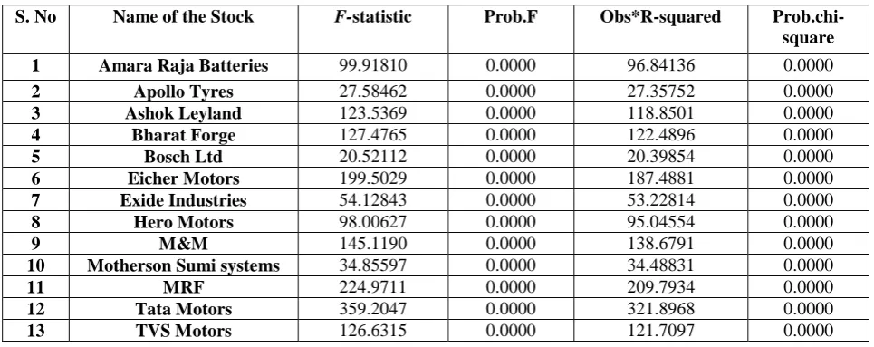
Before estimating volatility by using GARCH family models, it was necessary to identify whether there was substantial evidence for the presence of heteroscedasticity (ARCH effect) in the residuals of return series of the stocks selected for the study. In order to test whether the ARCH effect exists or not in the residuals of the return series, residual diagnostics test were conducted, which is lag range multiplier test for autoregressive conditional heteroscedasticity (ARCH) in the residuals and the results retrieved are shown in Table 3.In order to explore the most suitable model to specify the level of symmetric volatility of the selected stocks , GARCH models with various order like GARCH (1,1), GARCH (1,2), GARCH (2,1) and GARCH (2,2) were employed. In the process of selecting the best fitting model, as per the decision rule, the Akaike Information Criterion (AIC) and Schwarz Information Criterion values are taken into consideration along with the log likely hood value wherever need arises. The results obtained from these models are exhibited in Table no. 4 and the results revealed that the GARCH (1,1) is the most suited model. To find out the magnitude of symmetric volatility of the stocks selected for study, GARCH (1,1) model has been applied and the output from GARCH (1,1) model is exhibited in Table No. 5. To test the adequacy of the selected GARCH (1,1) model and to deduct whether ARCH effect exists or not in the residuals of the return series after the estimation of the GARCH (1,1) model, ARCH - LM test was conducted by using the residuals obtained after the application of GARCH (1,1) model. The obtained results from ARCH-LM test should show no evidence of remaining ARCH effect in the residuals, which is a necessary condition to indicate that the selected model is a perfect choice and has modeled the volatility pattern better than any other model. The results obtained from the ARCH - LM test is shown in Table No. 6.

In a financial market, if bad news has a more pronounced effect on volatility than good news of the same magnitude, such asymmetry has typically been attributed as Leverage

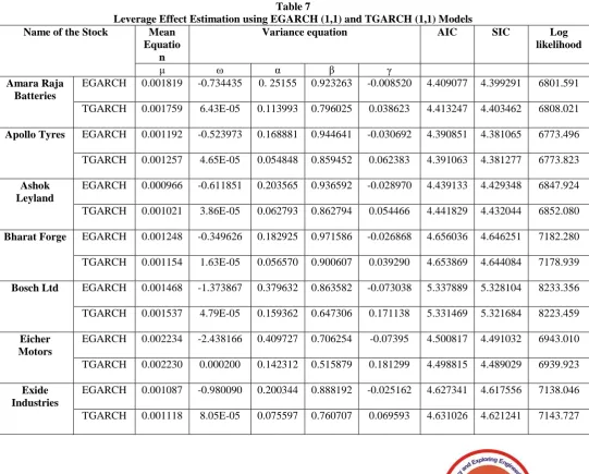
effect, and then the symmetric specification such as GARCH is not appropriate and could not capture the asymmetric effect, since only squared residuals enter the equation and the signs of the residuals or shocks have no effect (by squaring the lagged error in GARCH, the sign is lost) on the conditional volatility. In other words, the model assumes same effect for good and bad news. But, the fact of financial volatility is that negative shocks tend to have larger impact on volatility than positive shocks. The main drawback of the symmetric GARCH model is that the conditional variance is unable to respond asymmetrically to rise and fall in the stock returns. Hence to examine the asymmetric effect of the financial time series data, Exponential GARCH (EGARCH) and Threshold GARCH (TGARCH) model were applied. In order to account for the leverage effect observed in return series of the selected stocks, the asymmetric models which include EGARCH (1,1) and TGARCH (1,1) were employed and the results found from these two models are shown in Table No. 7.

IV.RESULTS AND DISCUSSIONS

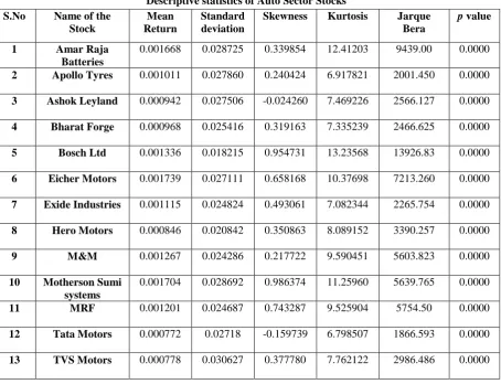
Table 1 presents the descriptive statistics of daily returns of the selected auto sector stocks of Nifty. The mean returns for all the 13 stocks are positive, indicating the fact that the prices of these stocks has increased considerably during the study period. Eicher Motors has delivered the highest return (0.001739) followed by Motherson Sumi Systems (0.001704) and Tata Motors (0.000772) and TVS Motors (0.000778) have delivered comparatively lower returns during the study period. The values of standard deviation are comparatively high for TVS Motors (0.030627) followed by Amara Raja Batteries (0.028725), Motherson Sumi (0.028692) and Apollo Tyres (0.027860) and it is low for Bosch Ltd (0.018215) and Hero Motors (0.020842). The descriptive statistics shows that the daily returns are positively skewed for all the stocks except Ashok Leyland (-0.024260) and Tata Motors (-0.159739) which explains that the return of these stocks increases more often than it decreases and there is a high probability of earning returns which is greater than the mean returns. The kurtosis data depicted in the table shows that all the stocks selected for the study are having K value greater than 3, which implies that the return series are fat tailed and they do not follow a normal distribution. This is further confirmed by the p values of Jarque Bera test statistics which are less than 0.05 (p<0.05).

Table 2 shows the calculated test statistic values (at level) for all the selected stocks of auto sector index of NSE using Augmented Dickey Fuller Test (ADF) and Philips Perron Test (PP). The test critical values for both ADF and PP test at 5 percent level are -2.862279 for the Test Equation-Intercept, -3.411264 for the Test Equation-Trend and Intercept and -1.94027 for the Test Equation-None and were compared with the calculated values. As per the decision rule to reject the null hypothesis that the variable has unit root problem, the calculated absolute test statistic values for all the stocks are much higher than the absolute test critical values and hence, the null

of selected stocks” is rejected with the conclusion that the return series of all the selected auto sector stocks are stationary in nature.

Table 3 exhibits the calculated coefficient values and the probability values of the stocks selected for the study and show that they are statistically significant and all the calculated F statistic values are higher than the observed R square values which is a necessary condition to reject the null hypothesis of „No ARCH effect in the return series. Hence it is proved that there is a heteroscedasticity - ARCH effect in the time series of the selected stocks and which requires the application of GARCH family models to understand the volatility in the stocks. The results of GARCH (1,1), GARCH (1,2), GARCH (2,1), GARCH (2,2) models for the selected stocks are presented in Table 4 for the purpose to select the best fit model to understand the nature of volatility. To select the best fit model, the AIC and SIC values were compared with each other and the model with minimum AIC and SIC value would be selected as the best fit one. Both the AIC and SIC values of GARCH (1,1) model were compared with the AIC and SIC values of all other models and was found that GARCH (1,1) model was the best fit model for all the selected stocks except Apollo Tyres and Bharat Forge. In both the cases, the AIC values of GARCH (1,1) is lower than remaining models but the SIC values of GARCH (1,1) model (4.379334 for Apollo Tyres and 4.643269 for Bharat Forge) are higher when compared with the GARCH (2,1) model (4.379315 for Apollo Tyres and 4.674128 for Bharat Forge). Hence, an additional parameter - the log likely hood value - has been taken into account to decide the best fit model. The log likely hood values, a parameter to decide when there is a tie, reveal that the GARCH (1,1) is the best fit model for both the stocks, as per the guidelines, since GARCH (1,1) is having the highest log likely hood values (6766.833 for Apollo Tyres and 8211.883 for Bharat Forge) when compared with the values of GARCH (2,1) model (6711.472 for Apollo Tyres and 8187.562 for Bharat Forge) .

Table 5 shows the estimates of the GARCH (1,1) model for all the selected stocks of auto sector of NSE. The values of all the parameters (ω, α and β) are positive, which satisfy the condition ω ≥ 0, α ≥ 0, β ≥ 0 to specify that the model is well defined to understand the volatility of the selected stocks. All the coefficients of lagged squared residuals (α) are positive and significant at five percent level showing that the news about previous volatility (past squared residuals term) has an explanatory power on current volatility. All the coefficient (β) values of lagged conditional variance are also positive and significant at five per cent level and specify that the past volatility of stock returns is significantly influencing current volatility. The sum of ARCH and GARCH coefficient (α + β) values, which is a measure of persistence of variance, of all the selected stocks of auto sector, is closer to unity (1) except Eicher Motors (0.723793), MRF (0.840342), Exide Industries (0.855111) and Bosch Ltd (0.891833) indicating that there is significant persistence in volatility. The large sum of these coefficient values implies that a large positive or a large negative return, which will lead future forecast of the variance to be high for a protracted period. The volatility persistence is very high in the case of Motherson Sumi Systems

(41.78395) followed by M and M (39.26760) and Bharat Forge (24.24454) implies that these stocks have experienced high level of volatility lasting for many days during the study period and the volatility persistence is low in the case of Eicher Motors (2.14430) and Exide Industries (4.42837) revealing very low level of volatility and is lasting for very short period of time. Table 6 exhibits the results obtained after applying the ARCH LM test from the residuals of GARCH (1,1) model for the selected stocks. Since all the calculated F statistics values are lesser than the observed R square values and the probability values are greater than 0.05 (p > 0.05), the null hypothesis of „No ARCH effect in the residuals‟ are accepted and confirms the absence of auto regressive conditional heteroscedasticity effect in the residuals of the return series after the estimation of GARCH (1,1) model.

Table 7 reports the results obtained from applying EGARCH (1,1) and TGARCH (1,1) model to capture the asymmetries in the return series of selected auto sector stocks of NSE. The calculated values from EGARCH (1,1) model reveal that the leverage effect exists in the selected stocks during the study period. The calculated values of ‘γ’ - which is used to notify the leverage effect, are negative and statistically significant (P values are less than 0.05) for all the stocks which expresses that negative shocks have more impact than the positive shocks on the volatility of the selected stocks. The calculated GARCH (β) values of all the stocks are positive and closer to unity (1) expressing the fact that the volatility persistence is explosive except Bosch (0.863582), Eicher Motors (0.706254), Exide Industries (0.888192) and MRF (0.804502). The results obtained from an alternative model - TGARCH (1,1) also confirm that the leverage effect is present in the auto sector stocks during the study period. As per the decision rule, the calculated coefficient values of ‘γ’ for all the stocks are positive and significant at 5 per cent level. The calculated GARCH values (β) from this model also confirm that the volatility is persistent during the study period except the stocks like Bosch (0.647306), Eicher Motors (0.515879), Exide Industries (0.760707) and MRF (0.674373). To select the best fit model to understand the leverage effect, the values of Akaike Information Criterion (AIC) , Schwarz Information Criterion (SIC) and Log likelihood for both EGARCH (1,1) and TGARCH (1,1) were compared with each other and was found that EGARCH (1,1) is the most suited one for the selected stocks, since the calculated AIC and SIC values from EGARCH (1,1) model are lower than the values from TGARCH (1,1) model except the stocks like Bharat Forge, Bosch, Eicher Motors and Hero Motors. But, to estimate the leverage effect of Bharat Forge, Bosch, Eicher Motors and Hero Motors, as per the guidelines, TGARCH (1,1) is the suitable model when compared with the other alternative models.

V. SUMMARY OF FINDINGS AND CONCLUSION

They are either positively or negatively skewed and the kurtosis values are greater than 3, which imply that the return series are leptokurtic in nature. The daily mean return of these stocks is positive and it is highest in Eicher Motors (0.001739) followed by Motherson Sumi Systems (0.001704) and lowest in Tata Motors (0.000772) and TVS Motors (0.000778).

o It is found from the results of Augmented Dickey Fuller test and Philips Perron test that the natural logarithmic values of daily return series of all the stocks selected for this study are stationary (at level) in nature. The calculated absolute test statistic values for all the stocks taken for the study are much higher than the absolute test critical values (McKinnon critical value) at 5 per cent level which reject the null hypothesis that the variable has unit root problem.

o The residual diagnostic tests conducted to find the presence of ARCH effect in the daily return series of all the selected stocks reveals that the ARCH effect exists in all the return series taken for this study. The calculated F-statistics values for all the selected stocks are well above the observed R square values and they are significant at one percent level. The null hypothesis is rejected and proves that the return series of all the stocks are having ARCH effect. This necessitates the application of GARCH family models to understand the volatility patterns of the selected stocks.

o In order to understand the best fit model to estimate the volatility pattern of the selected auto sector stocks, Akaike Information Criterion, Schwarz Information Criterion and Log likelihood values from the results of GARCH (1,1),GARCH (1,2),GARCH (2,1),GARCH (2,2) were considered and found as per the guidelines that GRACH (1,1) is the suited model for majority of the selected stocks.

o From the calculations of GARCH (1,1) model for auto sectoral stocks of NSE, it is found that there is significant persistence in volatility among these stocks except Eicher Motors, Exide Industries and Bosch Industries. The volatility persistence is very high in the case of Motherson Sumi Systems (41.78395) followed by M and M (39.26760) and Bharat Forge (24.24454) which implies that these stocks have experienced high level of volatility, lasted for many days during the study period and it is low in the case of Eicher Motors (2.14430), Exide Industries (4.42837) and Bosch industries (6.05493) which reveals very low level of volatility in these stocks and lasted for very short period.

o It is found from the ARCH-LM test conducted to find out the presence of heteroscedasticity in the residuals obtained after application of GARCH (1,1) model in all the selected stocks that there is no evidence of ARCH effect remaining in the return series. This is an indication of perfection of the model and there is no ARCH effect remaining that needs to be modeled by any other GARCH models.

o It is found that EGARCH (1,1) model is the most suited model to understand the leverage effect of all the selected stocks of auto sectoral index of Nifty except Bharat Forge, Bosch, Eicher Motors and Hero Motors. It is also found from the calculated values of EGARCH (1,1) model that the leverage effect exists in all the selected stocks

during the study period. The calculated values of „γ’are negative and statistically significant (P values are less than 0.05) for all the stocks which expresses that negative shocks have more impact than the positive shocks on the volatility of the selected stocks.

A. Conclusion

An attempt was made in this research work to frame a model for the volatility, leverage effect among the auto sectoral stocks of NSE-Nifty. The daily closing prices of selected stocks from April 2003 to January 2017 were collected and modelled by using GARCH family models. These models were employed in this research work after confirming the unit root test, volatility clustering and auto regressive conditional heteroscedasticity effect. While estimating the symmetric volatility, GARCH (1,1) model was found to be a better model and the same was employed to address the volatility persistence. The findings of this study reports that the Indian equity market exhibits the persistence of volatility and confirms that the majority of the selected stocks have experienced the high-level volatility during the study period. To investigate the presence of asymmetric volatility, the leverage effect needs to be assessed and henceforth, EGARCH (1,1) and TGARCH (1,1) models were employed. The results show that the coefficient has the expected sign both in the EGARCH (negative and significant) and TGARCH (positive and significant) models.

The findings of the study reveal that the leverage effect exists in the Indian equity market, where a negative shock causes more volatility than the positive one of the same magnitudes. In the process of selecting the best fitting model among these, to understand the leverage effect, AIC and SIC values were used and which proved that EGARCH (1,1) model is the best fitted model to capture the asymmetric volatility for majority of the selected stocks as per the AIC and SIC criterion. On a whole, this study concludes that Indian equity market is experiencing symmetric volatility and it is not insulated from leverage effect too. A negative nature of information to the market, delivers more volatility than the positive one of the same size. A study of this kind would be more useful to the budding investors, who invest their hard-earned money, in the equity market to understand the level of volatility in the market and to know how to stay in the bumpy and volatile market situations. A similar research may be conducted for short term period by considering intraday price behaviour with an hour interval, may throw a different view about the short-term volatility and may give a better insight about the presence of leverage effect during the intraday.

REFERENCES

1. Cheng F. Lee, Gong-Meng Chen and Oliver M Rui (2001) “Stock Returns and Volatility on China‟s Stock Market”, Journal of Financial Research, Vol.24, No.4, pp.523-543.

2. Des Nicholls and David Tonuri (1995), “Modeling Stock Market Volatility in Australia”, Journal of Business Finance & Accounting, Vol.22, Issue.3, pp.377-396.

3. James M Porterba and Lawrence H Summers (1986), “The Persistence of Volatility and Stock Market Fluctuations”, American Economic Review, Vol.76, No.5,

4. Karunanithy Banumathy and Ramachandran Azhagaiah (2015), “Modeling Stock Market Volatility: Evidence from India”, Spring, Managing Global Transitions, Vol.13, No.1, pp.27-42.

5. Kashif Saleem (2007),” Modeling Time Varying Volatility and Asymmetry of Karachi Stock Exchange (KSE)”, International Journal of Economic Perspectives, Vol.1, No.1, pp 01-09.

6. Kennth R French, G William Schewert and Robert F StanbaughR (1987) “Expected stock Returns and volatility”, Journal of Financial Economics, Vol.19, No.1, pp. 03-29.

7. Madhusudan Karmakar (2005) “Modeling Conditional Volatility of the Indian stock Market”, Vikalpa, Vol.30, No.3, pp. 21-37.

8. Olan Henry (1998), “Modelling The Asymmetry of Stock Market Volatility”, Applied Financial Economics, Vol.8, No.2, pp.145-153. 9. Pandey.A, (2005), “Volatility Models and Their Performance in

Indian Stock Market”, Vikalpa, Vol.30, No.2, pp.27-46.

10 Puja Padhi (2006), “Stock Market Volatility in India: A Case of Selected Scrips”, Indian Institute of Capital Markets 9 th _Capital

Conference Paper, Social Science Research Network, www. ssrn.com, id.873985.

11. Rakesh Kumar and Raj S Dhankar (2010), “Empirical Analysis of Conditional Heteroscedasticity in Time Series of Stock Returns and Asymmetric Effect on Volatility” Global Business Review, Vol.11, No.1, pp.21-31.

APPENDIX

Table 1

Descriptive statistics of Auto Sector Stocks

Table 2

Tests for Unit Root Problem in the Selected Stocks S.No Name of the

Stock

Mean Return

Standard deviation

Skewness Kurtosis Jarque Bera

p value

1 Amar Raja

Batteries

0.001668 0.028725 0.339854 12.41203 9439.00 0.0000

2 Apollo Tyres 0.001011 0.027860 0.240424 6.917821 2001.450 0.0000 3 Ashok Leyland 0.000942 0.027506 -0.024260 7.469226 2566.127 0.0000

4 Bharat Forge 0.000968 0.025416 0.319163 7.335239 2466.625 0.0000 5 Bosch Ltd 0.001336 0.018215 0.954731 13.23568 13926.83 0.0000 6 Eicher Motors 0.001739 0.027111 0.658168 10.37698 7213.260 0.0000

7 Exide Industries 0.001115 0.024824 0.493061 7.082344 2265.754 0.0000 8 Hero Motors 0.000846 0.020842 0.350863 8.089152 3390.257 0.0000

9 M&M 0.001267 0.024286 0.217722 9.590451 5603.823 0.0000

10 Motherson Sumi systems

0.001704 0.028692 0.986374 11.25960 5639.765 0.0000

11 MRF 0.001201 0.024687 0.743287 9.525904 5754.50 0.0000

S.No Name of The Stock

Augmented Dickey Fuller Test Phillips Perron Test Intercept Trend and

Intercept

None Intercept Trend and

Intercept

None

1 Amara Raja Batteries

-51.19818 -51.19032 -51.04818 -51.29797 -51.29022 -51.27846

2 Apollo Tyres -53.72203 -53.71375 -53.72203 -53.72203 -53.72203 -53.7220 3 Ashok Leyland -51.57045 -51.56250 -51.52195 -51.51887 -51.51078 -51.45096 4 Bharat Forge -52.83284 -52.82880 -52.76759 -52.84322 -52.83852 -52.83226

5 Bosch Ltd -53.72070 -53.74611 -53.45248 -53.71935 -53.74368 -53.45212 6 Eicher Motors -52.05687 -52.06257 -51.86724 -51.96234 -51.96562 -51.77720

7 Exide

Industries

-54.81009 -54.87267 -54.71672 -54.92512 -55.02456 -54.78809

8 Hero Motors -56.02681 -56.06389 -55.91015 -55.03066 -55.12894 -54.81628

9 M&M -50.27951 -50.32149 -50.16269 -50.04882 -50.08278 -49.96553

10 Motherson Sumi Systems

-58.83445 -58.83961 -58.62423 -59.14209 -59.15638 -58.76838

11 MRF -49.11891 -49.11175 -49.02719 -49.48886 -49.48095 -49.51659

12 Tata Motors -50.85450 -50.86399 -50.82539 -50.68314 -50.69148 -50.66795

13 TVS Motors -54.50612 -54.50756 -54.47741 -54.50332 -54.50714 -54.47987 (Test critical values @ 5% level is -2.862279 for Intercept; @5% level is -3.411264 for Trend and Intercept; @5%level is

-1.940927 for None, p values for all the above observations are < 0.05).

Table 3

Testing the Heteroskedasticity Effect in the Return Series of the Selected Stocks

S. No Name of the Stock F-statistic Prob.F Obs*R-squared

Prob.chi-square

1 Amara Raja Batteries 99.91810 0.0000 96.84136 0.0000

2 Apollo Tyres 27.58462 0.0000 27.35752 0.0000

3 Ashok Leyland 123.5369 0.0000 118.8501 0.0000

4 Bharat Forge 127.4765 0.0000 122.4896 0.0000

5 Bosch Ltd 20.52112 0.0000 20.39854 0.0000

6 Eicher Motors 199.5029 0.0000 187.4881 0.0000

7 Exide Industries 54.12843 0.0000 53.22814 0.0000

8 Hero Motors 98.00627 0.0000 95.04554 0.0000

9 M&M 145.1190 0.0000 138.6791 0.0000

10 Motherson Sumi systems 34.85597 0.0000 34.48831 0.0000

11 MRF 224.9711 0.0000 209.7934 0.0000

12 Tata Motors 359.2047 0.0000 321.8968 0.0000

13 TVS Motors 126.6315 0.0000 121.7097 0.0000

Table 4

Name of the stock GARCH (1,1) GARCH (1,2) GARCH (2,1) GARCH (2,2)

AIC SIC AIC SIC AIC SIC AIC SIC

Amara Raja Batteries 4.41266 4.40483 4.45137 4.40835 4.49375 4.41347 4.42746 4.40999 Apollo Tyres 4.38717 4.37933 4.39346 4.38546 4.41786 4.37935 4.39884 4.39665 Ashok Leyland 4.43849 4.43066 4.45448 4.44221 4.45448 4.43987 4.66735 4.44645

Bharat Forge 4.65192 4.64326 4.68356 4.69764 4.68356 4.67412 4.65119 4.66744 Bosch Ltd 5.32468 5.31678 5.33564 5.38734 5.39804 5.31895 5.33793 5.33687 Eicher Motors 4.49304 4.48521 4.49762 4.49832 4.49314 4.48553 4.49997 4.48772

Exide Industries 4.62877 4.62094 4.64145 4.66742 4.65365 4.65932 4.63778 4.62113 Hero Motors 4.97216 4.96433 4.99954 4.97349 4.98329 4.96442 5.01794 5.15597 M&M 4.80772 4.79989 4.89007 4.80648 4.89269 4.80032 4.90026 4.88472 Motherson Sumi Systems 4.41732 4.40949 4.48732 4.42675 4.49572 4.39991 4.43671 4.41166

MRF 4.69255 4.68472 4.71267 4.69463 4.78432 4.69532 4.95639 4.68995

Tata Motors 4.55360 4.54578 4.59854 4.57634 4.59955 4.55783 4.56633 4.55964 TVS Motors 4.24170 4.23396 4.29657 4.28623 4.29657 4.27648 4.25333 4.24479 *Log likely hood values - For Apollo tyres : 6766.833 and 6711.472 for GARCH (1,1) and GARCH (2,1) models respectively: For Bharat Forge : 8211.883 and 8187.562 for GARCH (1,1) and GARCH (2,1) models respectively.

Table 5

Volatility Estimation by Using GARCH (1,1) Model Name of the

stock

ω α β α + β SIC AIC Log

Likelihood

Volatility persistence Amar Raja

Batteries

6.21E-05 0.129979 0.800564 0.930543 4.404835 4.412663 6806.120

9.628783 ApolloTyres 3.55E-05 0.070940 0.886021 0.956961 4.379334 4.387177 6766.833

15.755980 Ashok

Leyland

2.75E-05 0.074520 0.891362 0.965882 4.430667 4.438496 6845.941

19.967594 Bharat Forge 1.88E-05 0.080640 0.891175 0.971815 4.643269 4.651920 7173.667

24.244543 Bosch Ltd 4.48E-05 0.222210 0.669623 0.891833 5.316780 5.324680 8211.883

6.0549360 Eicher

Motors

0.000208 0.208332 0.515461 0.723793 4.485211 4.493040 6930.020

2.144307 Exide

Industries

8.95E-05 0.116691 0.738420 0.855111 4.620948 4.628776 7139.258

4.428376 Hero Motors 2.30E-05 0.073296 0.875080 0.948376 4.964336 4.972164 7668.591

13.077204 M&M 1.02E-05 0.074693 0.907810 0.982503 4.799893 4.807721 7415.102

39.267608 Motherson

Sumi Systems

1.19E-05 0.032763 0.950785 0.983548 4.409498 4.417327 6813.309

41.783952

MRF 9.98E-05 0.166290 0.674052 0.840342 4.684723 4.692551 7237.568

3.9848336 Tata Motors 2.42E-05 0.084496 0.880475 0.964971 4.545780 4.553608 7023.386

TVS Motors 6.99E-05 0.113286 0.814004 0.927290 4.233962 4.241701 6542.720

9.182104 *All the values are significant at 5 per cent level

Table 6

Checking Adequacy of GARCH (1,1) Model Using ARCH – LM Test

S. No Name of the Stock F-statistic Prob.F Obs*R2

Prob.chi-square

1 Amara Raja Batteries 1.157432 0.2821 1.157748 0.2819

2 Apollo Tyres 0.155519 0.6933 0.155612 0.6932

3 Ashok Leyland 2.777363 0.0957 2.776663 0.0956

4 Bharat Forge 3.219049 0.0729 3.217776 0.0728

5 Bosch Ltd 0.203936 0.6516 0.204055 0.6515

6 Eicher Motors 0.018297 0.8924 0.018309 0.8924

7 Exide Industries 0.034018 0.8537 0.034040 0.8536

8 Hero Motors 1.867655 0.1718 1.867736 0.1717

9 M&M 1.372324 0.2415 1.372603 0.2414

10 Motherson Sumi Systems 0.824370 0.3640 0.824685 0.3638

11 MRF 1.060727 0.3031 1.061050 0.3031

12 Tata Motors 1.433493 0.2313 1.433757 0.2312

13 TVS Motors 1.327442 0.2494 1.327732 0.2492

Table 7

Leverage Effect Estimation using EGARCH (1,1) and TGARCH (1,1) Models Name of the Stock Mean

Equatio n

Variance equation AIC SIC Log

likelihood

μ ω α β γ

Amara Raja Batteries

EGARCH 0.001819 -0.734435 0. 25155 0.923263 -0.008520 4.409077 4.399291 6801.591

TGARCH 0.001759 6.43E-05 0.113993 0.796025 0.038623 4.413247 4.403462 6808.021

Apollo Tyres EGARCH 0.001192 -0.523973 0.168881 0.944641 -0.030692 4.390851 4.381065 6773.496

TGARCH 0.001257 4.65E-05 0.054848 0.859452 0.062383 4.391063 4.381277 6773.823

Ashok Leyland

EGARCH 0.000966 -0.611851 0.203565 0.936592 -0.028970 4.439133 4.429348 6847.924

TGARCH 0.001021 3.86E-05 0.062793 0.862794 0.054466 4.441829 4.432044 6852.080

Bharat Forge EGARCH 0.001248 -0.349626 0.182925 0.971586 -0.026868 4.656036 4.646251 7182.280

TGARCH 0.001154 1.63E-05 0.056570 0.900607 0.039290 4.653869 4.644084 7178.939

Bosch Ltd EGARCH 0.001468 -1.373867 0.379632 0.863582 -0.073038 5.337889 5.328104 8233.356

TGARCH 0.001537 4.79E-05 0.159362 0.647306 0.171138 5.331469 5.321684 8223.459

Eicher Motors

EGARCH 0.002234 -2.438166 0.409727 0.706254 -0.07395 4.500817 4.491032 6943.010

TGARCH 0.002230 0.000200 0.142312 0.515879 0.181299 4.498815 4.489029 6939.923

Exide Industries

EGARCH 0.001087 -0.980090 0.200344 0.888192 -0.025162 4.627341 4.617556 7138.046

Hero Motors EGARCH 0.000470 -0.715945 0.185474 0.925817 -0.004833 4.973372 4.963586 7671.452

TGARCH 0.000633 2.63E-05 0.070593 0.863205 0.014463 4.971703 4.961918 7668.880

M&M EGARCH 0.001213 -0.291911 0.163343 0.978167 -0.038121 4.807728 4.797943 7416.113

TGARCH 0.001228 1.17E-05 0.052128 0.903545 0.048232 4.811220 4.801435 7421.496

Motherson Sumi Systems

EGARCH 0.001294 -0.083409 0.054688 0.993963 -0.040822 4.424231 4.414445 6824.521

TGARCH 0.001369 5.03E-05 0.001456 0.972039 0.046886 4.433900 4.424114 6839.856

MRF EGARCH 0.001552 -1.697311 0.325794 0.804502 -0.008452 4.686143 4.676358 7228.689

TGARCH 0.001122 9.96E-05 0.165630 0.674373 0.001405 4.691904 4.682118 7237.569

Tata Motors EGARCH 0.000787 -0.314102 0.158738 0.973979 -0.035888 4.550028 4.540242 7018.868

TGARCH 0.000873 2.23E-05 0.053131 0.889752 0.049344 4.557469 4.547684 7030.339

TVS Motors EGARCH 0.000898 -0.812203 0.243017 0.910356 -0.014535 4.236354 4.226569 6535.340

TGARCH 0.000978 7.21E-05 0.104528 0.809090 0.024718 4.241691 4.231906 6543.567

* γ values are significant at 5 per cent level.

ASYMMETRIC VOLATILITY MODELING AND LEVERAGE EFFECT OF NIFTY STOCKS

AUTHORSPROFILE

MS. JINCY K. JOHN is full time Research Scholar in Department of Management Studies in Karunya Institute of Technology & Sciences, Coimbatore. She is having more than 10 years of experience in Banking Industry in India and Dubai. Last position held by her in Corporate sector was Senior Credit Evaluator in Mashreq Bank, Dubai. She completed her MBA from Department of Management Studies in Karunya Institute of Technology & Sciences, Coimbatore. She has presented more than three papers in National and International Seminars. Her area of interest is Share markets. She can be reached through [email protected] ,

Mob: 7397009124

DR. R. AMUDHA, is an Associate Professor in the area of Finance and the MBA Programme Academic Coordinator. She

has been a member of Coimbatore Management Association and has been the Editorial and review Board Member

of “Banking, Financial Services and Insurance” Book and reviewed International papers for „ICEHM‟ (International

Conference on Economics, Humanities and Management). She has been the Coordinator of the NCCMP course of NSE.

She is accredited trainer qualified with ADIFRS, UK and has also been instrumental in associating with IAAP (UK) to

introduce the IFRS course. She has published books on „Heuristics behavior of Investors in the Capital Market, Equity

analysis, Technical analysis. Visited several foreign countries for presenting her papers.