The Hensher equation: derivation, interpretation and implications for practical implementation

This is a repository copy of

The Hensher equation: derivation, interpretation and

implications for practical implementation

.

White Rose Research Online URL for this paper:

http://eprints.whiterose.ac.uk/87551/

Version: Accepted Version

Article:

Batley, R (2015) The Hensher equation: derivation, interpretation and implications for

practical implementation. Transportation, 42 (2). 257 - 275. ISSN 0049-4488

https://doi.org/10.1007/s11116-014-9536-3

[email protected] https://eprints.whiterose.ac.uk/ Reuse

Unless indicated otherwise, fulltext items are protected by copyright with all rights reserved. The copyright exception in section 29 of the Copyright, Designs and Patents Act 1988 allows the making of a single copy solely for the purpose of non-commercial research or private study within the limits of fair dealing. The publisher or other rights-holder may allow further reproduction and re-use of this version - refer to the White Rose Research Online record for this item. Where records identify the publisher as the copyright holder, users can verify any specific terms of use on the publisher’s website.

Takedown

If you consider content in White Rose Research Online to be in breach of UK law, please notify us by

1

The Hensher equation: derivation, interpretation and implications

for practical implementation

Richard Batley

Institute for Transport Studies, University of Leeds, UK

Abstract

The ‘Hensher equation’ is a prominent method for valuing the benefits of business travel time savings. This paper derives the equation from first principles, revealing several underpinning assumptions, as follows: a) production is a function only of labour given fixed capital; b) the value of the marginal product of labour is equal to the wage; c) business travel has constant productivity whether it takes place during work or leisure; and d) utility is a function of work, leisure and travel time. Informed by this derivation, the paper interprets the features of the resulting valuations. Finally, the paper also derives restricted and extended cases of the Hensher equation, applicable to a range of practical situations where the equation might be implemented.

Correspondence address: Dr Richard Batley, Institute for Transport Studies, University of Leeds, Leeds, LS2 9JT, United Kingdom; Telephone: +44 (0) 113 343 1789; Fax: +44 (0) 113 343 5334; E-mail: [email protected]

Keywords: Hensher equation, business travel time savings, value of the marginal product of labour.

2

The Hensher equation: derivation, interpretation and implications

for practical implementation

1. Introduction

According to conventional microeconomic theory, savings in business travel time may derive benefits to both the firm/employer and employee. From the point of view of the firm, time savings may facilitate:

a) additional work time at home or at the normal place of work; and/or b) additional or longer business trips;

both of which may potentially realise an improvement in the firm’s productivity. From the point of view of the employee, time savings may facilitate:

c) additional work time at home or at the normal place of work; and/or d) additional leisure time at home; and/or

e) re-timing of the business trip;

all of which may potentially realise an improvement in the employee’s utility. A number of approaches have been adopted for estimating the potential benefits listed above, the predominant ones being the so-called ‘cost savings’ and ‘Hensher’ approaches.

The cost savings approach (CSA) focuses upon benefit source a) above, and is underpinned by the following five assumptions (Harrison, 1974):

1. Competitive conditions in the goods and labour markets. 2. No indivisibilities in the use of time for production. 3. All released time goes into work, not leisure. 4. Travel time is 0% productive in terms of work.

3

If these assumptions hold, then cost savings arise from the direct compensation/reward to the employee, plus any additional costs of employing staff. On this basis, the CSA is often referred to as the ‘wage plus’ approach, and the value of business travel time savings (

VBTTS

) is formalised:

VBTTS w k

 

(1)

where:

w

is the gross wage;

k

is the non-wage cost of employing labour.

Despite widespread acceptance that the five assumptions detailed above are rather limiting, the CSA has been adopted within the official transport appraisal methods of a number of countries. A notable example is the UK Department for Transport, which has justified the approach with the following assertion: ‘Time spent travelling during the working day is a cost to the employer’s business. It is assumed that savings in travel time convert non-productive

time to productive use and that, in a free labour market, the value of an individual’s working

time to the economy is reflected in the wage rate paid. This benefit is assumed to be passed

into the wider economy and to accrue in some proportion to the producer, the consumer and

the employee, depending on market conditions’ (Department for Transport, WebTAG Unit 3.5.6).

The Hensher approach represents a comprehensive body of theoretical and conceptual ideas, supported by empirical evidence, on the value to society of savings in business travel time. The initial research arose from David Hensher’s engagement as a sub-contractor to consultants Travers Morgan, and the substantive theory and concepts were outlined by Carruthers & Hensher (1976)1, before being developed more fully and definitively by Hensher (1977). Influenced by Hensher’s formulation of

VBTTS

(see the working on pages

1

This paper was written by Hensher, as a I H 1976 book on the value of time and

4

169 to 171 of Carruthers & Hensher (1976) for example), Fowkes et al. (1986) proposed an alternative formulation focussed upon selected elements of Hensher’s approach, as follows2:



1





1



VBTTS

 

pq r MPL MPF





 

r VW



rVL

(2)

where:

p

is the proportion of business travel time saved that would have been spent working;

q

is the productivity of working whilst travelling relative to at the workplace;

r

is the proportion of business travel time saved that is allocated to leisure;

MPL

is the value of the marginal product of labour;

MPF

is the value of extra output due to reduced travel fatigue;

VW

is the difference between the employee’s valuations of ‘contracted’ work time and travel time.

VL

is the difference between the employee’s valuations of leisure time (i.e. the residual time given the work contract) and travel time.

Reflecting the provenance of the theoretical and conceptual ideas, (2) is commonly referred to as the ‘Hensher equation’. Mackie et al. (2003) remarked that: ‘In practice, Hensher

(1977) omitted

MPF

from his calculations, no doubt because of the difficulty of obtaining

suitable data, and this term has generally been ignored’ (p6). We will adopt the same

convention here, and focus the subsequent discussion on the slightly simplified specification:



1





1



VBTTS

 

pq r MPL



 

r VW



rVL

(3)

In contrast to the CSA, the Hensher equation (3) considers benefit sources a), c) and d) and thus combines the perspectives of the employer and employee. To these ends, the Hensher equation relaxes assumptions 3, 4 and 5 detailed above, and might therefore be seen as a

2

Whilst (2) focuses upon specific costs and benefits of business travel to the employer and employee,

H costs and benefits to both parties as well as to society more

generally. Note that, on the basis of the subsequent derivation of (2) from first principles in section 4, we have

5

behavioural valuation of business travel time savings, as distinct from the resource valuation given by the CSA. Although the Hensher equation has found conceptual appeal, practical implementation of (3) has proved difficult. Wardman et al.’s (2013) comprehensive review of the value of business travel time savings noted that Sweden (Algers et al., 1995) and The Netherlands (Significance et al., 2013) currently employ a restricted version of (3), whilst Norway previously advocated a similar specification before reverting in 2010 to the CSA. In particular, Wardman et al. reported: ‘We have not uncovered use of a full Hensher model...’ (p8). The restricted specification adopted in Sweden and The Netherlands was first proposed by AHCG (1994), and is given by the following:



1



VBTTS

 

pq r MPL VP





(4)

where

VP VW





VL

.

As Mackie et al. (2003) acknowledged, an alternative restriction on (2) is where

p r

 

0

and

VW



MPF



0

; provided adjustment is made for the non-wage cost of employing labour, the Hensher equation will in this case collapse to the CSA (1).

Against this background, the principal contributions of the present paper will be as follows:  Informed by similar work by previous authors, we will derive the Hensher equation

from first principles.

 This derivation will reveal new insights on the Hensher equation, in relation to its

underlying properties and intuition.

 Given the recent revival of policy interest in the Hensher equation, stimulated by

proposed major schemes such as High Speed 2 in the UK (HS2 Ltd., 2013)3, we will consider several variants of the equation relevant to specific practical situations.

3

6

2. Previous literature

Guided by Hensher’s substantive theoretical and conceptual ideas (Carruthers & Hensher, 1976; Hensher, 1977), Fowkes et al. (1986) proposed equation (2) – which is now commonly referred to as the ‘Hensher equation’ – but did not show its derivation from first principles. Of similar vintage to Fowkes et al. is Working Paper 3 from the 1987 UK national non-work VTTS study (MVA, ITS & TSU, 1987), which defined an optimisation problem ‘...on the lines

of Hensher’ (p72), but did not proceed to solve the problem. This gap in the literature

motivated the recent contributions of Karlström et al. (2007) and Kato (2013); the former derived an equation similar to (2), whilst the latter derived (2) exactly.

Karlström et al. (2007) generalised Hensher by distinguishing between short distance and long distance trips; the latter were defined as trips where it would not be feasible to return to the normal place of work at the end of the day. They further distinguished between private and social valuations of travel time savings, where social valuations account for the incidence of tax (e.g. Forsyth, 1980). In order to permit direct comparison against the Hensher equation, let us consider a restricted case of Karlström et al. involving a single short distance business trip subject to zero taxation4. On this basis, Karlström et al.’s optimisation problem entails the following key features:

 The problem is defined in terms of a ‘social planner’ model. In support of this conceptualisation, Karlström et al. suggested that ‘...it might be useful to think of the

individual under study as a “one-man firm”, making no distinction between the

interests of the firm and the interests of the individual’ (p4).

4

7

 More specifically, the objective statement is one of maximising utility, which is a

function of goods and time, subject to budget, time resource and time consumption constraints.

 

 

 

 

ˆ, , , , ,

ˆ

Max , , , , ,

s.t. ˆ

ˆ _{, , ,}

o d w w l w l

o d

w w l w l X T T T t t

o d

l w w w l w o d

w w l w l

w w w

l l l

W U X T T T t t

X c f T T t t c Y

T T T t t T

t t t t









         _{ }         (5) where:

W is social welfare

 

U



is the utility function of the individual;

ˆ

X

is the value of goods consumed;

o w

T is the quantity of work time spent at the normal place of work (or ‘origin’);

d w

T is the quantity of work time spent at other places of work (or ‘destination’);

l

T

is the quantity of leisure time;

w

t is the quantity of travel time to other places of work (i.e. business travel time), and

t

_w

is the minimum such travel time;

l

t is the quantity of travel time to the normal place of work (i.e. commuting time), and

t

_l

is the minimum such travel time;

l

c is the cost of commuting;

 

ˆ

f



is a function representing the value of the total product of labour;

w

c is the cost of business travel;

Y

is non-wage income;

8



is the marginal utility of income;



is the marginal utility of time;

w



is the marginal utility of the time consumption constraint for business travel;

l



is the marginal utility of the time consumption constraint for commuting.

Karlström et al. derived (in essence)5 the following equation for the value of business travel time savings:

ˆ ˆ

w

w w w w w

f T f

U U

VBTTS

T t



T t t

      

_  _  

    

  (6)

where T_w T_woT_wd.

Referring back to (5), this would seem to imply a restriction on the optimisation problem such

that



_w





_l



0

(i.e. neither of the time consumption constraints is binding). Whilst (6) is not equivalent to (2) – indeed there is no explicit specification of the

p

,

q

and

r

terms – it does embody some features of the Hensher equation, in particular the aggregation of ‘employee’ and ‘employer’ benefits. Karlström et al. observed that (6) reduces to the CSA (1) where the following three conditions hold: the entire travel time saving is converted to work (

1

w w T t

    ); the marginal utilities of work and business travel are equal (

w w

U T U t

    ); and the wage rate is equal to the value of the marginal product of labour.

Kato (2013) adopted Karlström et al.’s definition of short and long distance trips (although we will again focus on the former), and considered several variants of an optimisation problem, depending on whether business travel time is productive, and whether overtime is paid for

5

9

business travel time outside of normal working hours. Rather than cover all of these variants here, we will simply summarise the essence of the problem.

 Following Hensher (1977)6, the problem is defined in terms of a ‘collective’ model, which conflates the welfare accruing to both the employee and employer. In support of this conceptualisation, Kato asserted that: ‘If it is assumed that business activities

are generally implemented under the condition of Pareto efficiency in a group

consisting of an employer and employees, the collective model approach might be

the most preferable’ (p6).

 More specifically, the objective statement is one of maximising welfare, which is

additive in producer and consumer surplus, subject to budget, time resource and time consumption constraints7.









 

















 

 

 

* *

ˆ, , , ,

*

*

Max 1 ,

ˆ_{, 1 , , ,}

s.t. ˆ

w l w l

w w w w w w

X T T t t

w w l w l

l w

w l w l

w w w

W P f T r t p t g t wT c Y

U X T r t T t t

X c wT Y

T T r t t T

t t







    _   _       _   _         (7) where: *

p

is the proportion of business travel time that is spent working; this should be

distinguished from the

p

term in (2) which relates to travel time saving specifically;

*

r

is the proportion of business travel time that takes place during leisure time; this

should be distinguished from the

r

term in (2) which relates to travel time saving

specifically;

P

is the market price of goods produced;

6

Indeed, Hensher (1977) considered not only the benefits and costs of business travel to the employer and

7

10

 

f



is a function representing the total physical product of labour, wherein work and business travel time yield positive marginal productivity;

 

w

g t

is a function representing the total physical product of labour, wherein business

travel time yields negative marginal productivity (this appeals to the specification of the

Hensher equation (2) which includes the MPF term); and all other notation is as defined previously.

Unlike (5), it can be shown that the optimisation problem (7) yields the Hensher equation (2) exactly. To this end, Kato’s paper represents a notable contribution to the literature, and we will follow the essence of his approach in what follows. However, (7) is complicated, and includes a number of superfluous terms (for example, the contribution to the employee’s utility from leisure travel is irrelevant to the derivation of

VBTTS

). The subsequent discussion will draw from both Karlström et al. and Kato, but present a simpler derivation

focussed upon the Hensher equation (3), i.e. where

MPF



0

. This exercise will clarify the intuition behind (3), and expose several assumptions and properties which have not hitherto been fully articulated in the literature.

3. Specifying the optimisation problem behind the Hensher equation

In what follows, we will outline an optimisation problem wherein:

 The problem is defined in terms of the joint interests of the employer and employee.

 More specifically, the objective statement is one of maximising welfare, where

11





 

, , , * * Max s.t.

, , , 0

for , 0; 0 1; 0; 0 1

w l w w

X T T t

w l

w l w

W PX wT U

T T T

X T T t

p q r





 

            (8) where:

  







* * * *



1

1

w w

X



f T



_



r

p q

 

r



p q t



_



*



*

, ,

w w l w w UU T_ r t T r t t _

and8:

*

p

is the proportion of business travel time that is spent working;

q

is the productivity of working whilst travelling relative to at the workplace;

*

r

is the proportion of business travel time that takes place during leisure time;

W

is social welfare;

P

is the market price of goods produced/consumed;

X

is the quantity of goods produced/consumed;

w

is the market wage rate;

w

T

is the quantity of ‘contracted’ work time;

 

U



is the utility function of the employee;

 

f



is a function representing the total physical product of labour;

w

t

is the quantity of business travel time (which could straddle ‘contracted’ work and leisure time);

l

T

is the quantity of leisure time, given the work contract;

T

is the total time devoted to ‘contracted’ work and leisure (i.e. 24 hours in any one day);

8

12



is the marginal utility of income;



is the marginal utility of time.

It is important to understand the salient features of the optimisation problem, as follows:  With reference to the

W

function, we assume that revenue is generated through

the sale of goods, that costs are incurred through the employment of labour, and that both goods and labour markets are perfectly competitive. For simplicity, we further assume that the non-wage costs of employing labour are zero (i.e. with reference to

(1), we assume that

k



0

)9, and omit explicit consideration of tax (i.e. implicitly we assume that the taxation regime is neutral between employer and employee). These assumptions can be relaxed, albeit with a modest increase in complexity10.

 With reference to the

X

function, production depends solely upon the time contributed by the labour input, adjusted for the productivity of this time. In effect, this constitutes a short run production position where the firm’s capital is fixed. Productive time could, conceivably, include not only ‘contracted’ work time, but also a proportion of leisure time, hence the notion of ‘effective’ work (and leisure) time11. Note that, in contrast to Karlström et al. (2007) and Kato (2013), we specify a one-to-one

relationship between consumption and production, i.e.

X

 

f

 

.

 With reference to the

U

function, utility depends upon the quantities of ‘effective’ work time, ‘effective’ leisure time and business travel time (but not the consumption of goods; we will comment further on this feature in the subsequent discussion).  With reference to the



constraint, the time resource constraint is ostensibly the

sum of ‘contracted’ work and leisure time.

9

In practice, there may be savings in overheads from travelling instead of spending equivalent time in the workplace, but these are not considered here.

10

For example, section 7 of the present paper extends the analysis to consider taxation (see Case 6) and imperfect competition (see Case 7).

11

On this issue, Hensher (1977) remarked: W the

opportunity cost of an average hour of working time to the employer is traditionally assumed to be zero.

H

13

 With reference to the

p

*,

q

and

r

* parameters:

 We assume that these parameters are fixed, reflecting the contract between

the employer and employee, and are not subject to optimisation.

 Business travel time may straddle ‘contracted’ work and leisure time (hence the

*

r

term, and the notion of ‘effective’ work time).

 Business travel time may be less than fully productive (hence the

p

* and

q

terms)12. Although business travel time may straddle ‘contracted’ work and leisure time, we assume that

p

* and

q

are constant throughout the journey. In other words, the productivity of business travel is assumed constant, irrespective of whether business travel takes place during ‘contracted’ work or leisure time.

In contrast to conventional work-leisure optimisation problems such as Becker (1965), Oort (1969) and DeSerpa (1971), (8) omits an explicit budget constraint. This reflects the following assumptions:

 The employer and employee face a common marginal utility of income.

 Revenue from the sale of goods straightforwardly transfers to the wage-related

income of the employee.

 Non-wage income to the employee is zero.

Since labour costs already feature in the objective statement, and we have assumed zero non-wage income, there is no need to also include a budget constraint13. In passing, note

12_W

of empirical evidence concluded that p* is typically less than 0.3, whilst q

is typically close to 1.

13

In the vein of Karlström et al. (2007), an alternative (but equivalent) way of specifying the problem (8) would be to include a budget constraint, but represent the objective statement entirely in terms of the employee, as follows:

 

 

, , ,

Max

s.t. w l w X T T t

w

w l

W U

PX wT T T T

 





 

14

that wage-related income refers to ‘contracted’ work time

T

_w only; no wages are paid or received for business travel that takes place during leisure time r*t_w14

. Furthermore, in

contrast to DeSerpa, (8) omits an explicit technical constraint linking time and goods. This is because the inter-relationship between time and goods is already represented within the production function. For a practical illustration of the optimisation problem (8), see Figures 1 and 2.

Figure 1: ABOUT HERE

Figure 2: ABOUT HERE

4. Solving the optimisation problem

We will assume that the market prices of goods and labour (denoted P and

w

,

respectively) are determined exogenously, as is the marginal utility of income (



). On this basis, the optimisation problem (8) gives rise to four first-order conditions (9) to (12). The condition (9) solves for the quantity of goods produced. The condition (10) solves for the quantity of ‘contracted’ work time, which will be a determinant of both the firm’s output and the employee’s income.‘Contracted’ work time itself arises from the equilibrium between the employer’s demand for hours and the employee’s supply of hours. The latter provokes a trade-off between work and leisure, giving rise to the condition (11) which solves for the quantity of leisure time. Finally, the condition (12) solves for the quantity of business travel time, which will combine with the quantity of ‘contracted’ work time in determining the firm’s output.



w





w l



L U  PXwT  T T T

14

This resonates with the argument, advanced by Carruthers & Hensher (1976), that:

while travelling represents work that would be done I

15

0

W

P

X





_

_



(9)

 

 





w w w

W dX U

P w

T



d T T





   

 _{ }  _{ }

      (10)

l l

W

U

T

T



 



_



_



  

(11)

 

 





0

w w w w w

W dX U U U

P

t



d t t t t

     

   

    

          (12)

In principle, the value of business travel time (

VBTT

) is given by:

w

W

VBTT

t









As we will demonstrate, the Hensher equation arises from a distinct focus on the difference between the values of ‘contracted’ (and fully productive) work time

T

_w and business travel

16

 

 

 







1 1 1 1 w w w MPL w w VW VL

w w w

Vot w W W VBTTS T t dX P w

d T t

U U

T t t

U t













      _  _           _  _  _  _           _  _   _  _       where:

MPL

is the value of the marginal product of labour;

VW



is the value of ‘effective’ work time to the employee (we will explain the terminology in subsequent discussion);

VL



is the value of ‘effective’ leisure time to the employee;

w

Vot

is the value of business travel time to the employee.

Continuing with our derivation:

 





  















* * * *

* *

1 1 1

1

1

1

w

dX

VBTTS P r p q r p q w

d U U r r U t





        _{ }   _   _          Simplifying:

 











* * * * 2 1 1 1 w dX

17

Finally, if

MPL w



then we can further simplify to the following, which (as we will demonstrate below) is equivalent to (3):

 











* *

* *

1

1

1

1

w

dX

VBTTS P p q r d

U U

r r

U t





  



 _{ } 

 _   _

   

 

 



(14)

The above analysis reveals a number of properties arising from (8) which can now be summarised:

 The Hensher equation (14) is no different to the CSA in assuming that the value of

the marginal product of labour is equal to the wage rate, i.e.

MPL w



15

.

 Drawing reference to (3), (14) implies that p*p and r*r , meaning that no distinction is made between the average and marginal impacts of business travel time savings on both productivity and utility.

 If the first order condition (9) holds and



0 then

MPL



0

; in other words, resources will be allocated such that there is no marginal benefit to the firm/employer from additional production, and any benefits from business travel time savings will accrue solely to the employee.

 If

MPL w



and the first order conditions (10) and (11) hold then

w l

U T

U T



     

. Given the formulation of the

U

function in (8), the

implication follows that

       

U



U



16.

15

Section 7 of the present paper extends the analysis to consider possible discrepancy between the value of the marginal product of labour and the wage rate (see Case 7).

16

This is because  U T_w  U      

 

T_w where   



Tw 1, and similarly for leisure time. More

18

 If (9) holds then (12) simplifies to   U t_w r*



      U U





. If (10) and (11) also hold and

MPL w



then the first order condition (12) must itself hold. Otherwise, if

MPL w



or the first order conditions (9), (10) or (11) fail to hold then

w

U t

 

could be positive or negative.

Returning to our earlier comment regarding the technical constraint, it is notable that – aside from the introduction of the

p

*,

q

and

r

*parameters – the first order condition (10) is essentially the same as equation (21) in Jara-Díaz (2003), which was motivated by DeSerpa (1971), Evans (1972) and Oort (1969). Jara-Díaz remarked: ‘Note that [equation (21)] is a new (expanded) interpretation for the value of work, including the wage rate, the value of its

marginal utility and the technical impact of the work duration on goods consumption’

(p256)17.

Finally, it is appropriate to demonstrate the equivalence between (14) and (3), a matter which was clarified through private communication with Hironori Kato. With reference to

footnote 16, Kato pointed out (quite rightly) that if

  

U



is substituted with

 

U T

_w, and

U

  

with

 

U T

_l , then (14) can be re-stated:

 









 





* * * *

* * *

1 1

1 1

1 1

w l w

w w l w

dX U U U

VBTTS P p q r r r

d T T t

dX U U U U

P p q r r

d T t T T







    

    _   _

 _  _ 

       

    _  _{ }  _{ }

 _  _{ }  _{ }

(15)

Equation (15) can be further re-stated as follows, which allows simplification to (3):

-earning) hours remain constant, which would call for a non-linear functional form for utility.

17

19

 





 









* * * *

* * * *

1

1

1

1

1

1

w w l w w w

VW VL

MPL

w w l w

dX

U

U

U

U

U

U

VBTTS

P

p q r

r

r

d

T

t

T

T

t

t

dX

U

U

U

U

P

p q r

r

r

d

T

t

T

t















 

























_

_

_



_{ }





_

_

_



_



_



_

_





_{ }





_

_

_





_

























_



_





_



_



_





_

_





_

(16)

5. Further insights on the intuition behind the Hensher equation

Equation (14) represents an alternative (but equivalent) statement of (3), and exposes the following insights on the intuition behind the Hensher equation.

With regards to work time, we might distinguish between ‘contracted’ work time

T

_w and ‘effective’ work time





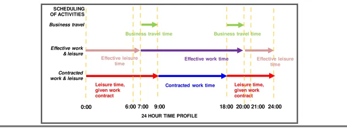
, where the former refers to income-earning hours only, whilst the

latter refers to income-earning hours plus any business travel undertaken during leisure time (i.e. outside of income-earning hours). With reference to Figure 1, for example, ‘effective’ work time comprises 9 hours ‘contracted’ work time plus 6 hours business travel time. Given this distinction, the term VW    



U







in (14) can be interpreted as the value of ‘effective’ work time, and the factor



1



r

*



represents the proportion of business travel time

that falls within ‘contracted’ work time. On this basis, we can also reason that the ‘effective’ wage rate w w T



_w



T_w r t* _w





will be less than or equal to the ‘contracted’ wage rate

w

. Moreover, the term

VW

 



1

r

*



as a whole represents the value to the employee of retaining business travel time savings as ‘effective’ work time (i.e. outcome 1 in Figure 2).

With regards to leisure time, and in a similar vein to the discussion above, the term





20

employee, and the factor

r

* represents the proportion of business travel time that, given the work contract, falls within leisure time. Moreover, the term

VL r



* as a whole represents the value to the employee of transferring business travel time savings into ‘effective’ leisure time (i.e. outcome 2 in Figure 2).

Having interpreted

VW



and

VL



, the collective term

VW



 



1

r

*





VL r





* represents the total value of business travel time savings to the employee, accounting for the possibility that such savings could be allocated to ‘effective’ work or leisure. Moreover, this distinction between ‘effective’ work and leisure exposes the crucial role played by the

r

* parameter within the Hensher equation; see Wardman et al. (2013) for a comprehensive review of empirical evidence on this (and the other) parameter(s) of (14).

The derivation of the Hensher equation in section 4 above also reveals insights on the intuition behind (4), which was the restricted specification employed in the Swedish and

Dutch national

VBTTS

studies. Justifying this specification, Algers et al. (1995) asserted: ‘In

this study, the value of time to the employee was not differentiated depending on whether

the time saved would be spent at work or on leisure, and it was thus implicitly assumed that

the private VOT (VP) is the same in both cases, or that VW equals VL’. (p142). Rationalising

this specification in the context of (16), note that if

MPL w



and the first order conditions (10) and (11) hold, then

    

U T

_w

U T

_l and (16) simplifies to:

 



1

* *



1

VW

w w

dX

U

U

VBTTS

P

p q r

d



T

t

















_



_



_





_

Mackie et al. (2003) subsequently challenged this assertion: ‘Setting VW to VL implies that

the marginal utility to the employee of time in work is assessed equal to that spent in leisure.

21

VL, since travellers will not be indifferent between spending time working and leisure time.’

(p13). That is to say, Mackie et al. questioned whether the first order conditions (10) and (11) will in practice hold.

6. Restricted cases of the Hensher equation

Having derived the Hensher equation from first principles, let us now consider some restricted cases of (16)18.

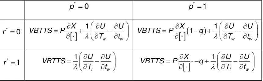
Case 1: Bates (2007)

Bates (2007) considered all four permutations of the limiting values of

p

* and

r

*. These permutations differ in terms of whether productive (

p

*



1

) or unproductive (

p

*



0

) travel time is saved, and whether this time is transferred to productive time in the workplace (

*

0

r  )19 or to leisure time (

r

*



1

)20.

Table 1: ABOUT HERE

Case 2: Wardman et al. (2013)

If we assume (perhaps not unreasonably) that

VW



0

, meaning that the employee is indifferent between ‘contracted’ work time and business travel time, then we derive the restricted case of (16):

 



1

* *



1

*

VL

l w

dX

U

U

VBTTS

P

p q r

r

d



T

t

















_



_



_





_

(17)

18

For reasons of brevity, subsequent cases will not present full working but simply the final derivation of

VBTTS in each case.

19

Note that r*0 corresponds with the first o F

20

Note that *

1

22

Describing this as the ‘most typical formulation’ of the Hensher equation, Wardman et al.

employed this as the basis for their empirical comparison of

VBTTS

from the cost savings, Hensher and willingness-to-pay (WTP) approaches. According to (17), the employee’s valuation of business travel time savings depends solely upon the difference between his/her valuations of ‘contracted’ leisure time and business travel time. A common practice is to assume

VL VTTS



, where

VTTS

is the value of non-work travel time savings; in the

limiting case where

p

*



0

and

r

*



1

, this assumption implies that

VBTTS VTTS



.

Case 3: Cost savings approach

Continuing with (17), consider the assumption

VL w



, which corresponds to the case where overtime is paid at the standard wage rate for any business travel undertaken during ‘contracted’ leisure time21

. Remembering that

MPL w



, if we discount productivity issues (

*

0

p



) and the non-wage costs of employing labour (

k



0

), then the assumption

VL w



implies that

VBTTS



w

, i.e. (17) collapses to the CSA (1). An alternative rationale for

deriving (1) from (17) is to note that, in the case of ‘flexible’ work contracts where the employee is hired on demand and paid for any hours worked22, business travel takes place entirely within ‘contracted’ work time (r* 0). If, in this case, we discount productivity issues and the non-wage costs of employing labour, then (17) again reduces to the CSA (1). Whilst these limiting cases offer useful theoretical insight, we should however acknowledge Wardman et al.’s (2013) finding – based on comprehensive international evidence – that empirical estimates of

VBTTS

using (17) are generally lower than those from the CSA. This implies that the limiting cases do not occur in practice.

21

A premium overtime rate would call for a further adjustment.

22

23

7. Extended cases of the Hensher equation

Whereas section 6 considered restricted cases of (16), let us now consider potential extensions to the Hensher equation, which involve either relaxing the underpinning assumptions, or introducing additional elements. As the basis for this discussion, we will revert to the more general statement of the Hensher equation (14).

Case 4: Business travel time is less productive during leisure time

As noted in section 3 above, the Hensher equation implicitly assumes that business travel which takes place during leisure time is equally as productive as business travel that takes place during ‘contracted’ work time. If business travel during leisure time is, in practice, less productive then (14) will understate the benefits of business travel time savings. Taking the extreme case where business travel during leisure time is entirely unproductive, we derive the following:

 



1 * * * *



1





1 *



* 1 w

dX U U U

VBTTS P p q r r p q r r

d





t

    

 _     _{ }  _{ } _ _

 

Case 5: Business travel has a broader productive benefit for society

The Hensher equation assumes that labour is the sole input to production and, apart from productivity issues, plays the same role whether in situ at the workplace or in transit; this

assumption gives rise to the production function

X

 

f

 

in (8). If, in practice, the productive

contribution of business travel is not simply one of labour input, but a broader one of generating and/or facilitating production (e.g. by visiting clients or suppliers), then there is a

case for extending the production function to

X

  

f

   

g t

_w , where

f

 



is defined as

before and

g t

 

_w is a separate functional relationship between output and business trips.

24

 

 



1

* *



 

ww

1





1

*



*

1

w

df

dg t

U

U

U

VBTTS

P

p q r

r

r

d

dt





t





















_









_





_







_





_

 

 

_







(18)

Since savings in business travel time would allow more business trips to be carried out, or allow more meetings to be conducted on a given business trip, we would expect

 

_{w w}

0

dg t

dt



23

. That is to say, the

g t

 

_w function would bring additional benefits of travel

time savings to complement those already captured by the

f

 



function. This proposition

resonates with Kato’s optimisation problem (7) which features two production functions; one where business travel time has a negative impact on productive output (although he

attributed this to fatigue on the part of the employee, i.e. the MPF term in (2)), and a

second where business travel time has a positive impact on productive output (i.e. the MPL

term).

Case 6: Business travel time has tax implications for employee and employer

Forsyth (1980) argued that, in the context of appraisal, neither the market wage rate (i.e. pertaining to work) nor the marginal value of leisure time (i.e. pertaining to non-work) represent the correct value of time in a taxed economy. Motivated by this argument, we can

straightforwardly extend (13)24 to take account of differential rates of taxation on sales

 



_P and income

 



_w .



₁



_{ }



₂ * *





₁



1

_



₁ *



* 1

P w

w

dX U U U

VBTTS P p q r w r r

d t









 _{ }  _

       _   _

 _    _ 

(19)

23

There is a question as to the applicability of the behavioural value (18) to the social value of travel time savings in appraisal, since the latter is concerned with the marginal value of labour productivity and/or the resource value of labour released into the market, but not the marginal value of the trip.

24

25

If



_P





_w then (13) holds, otherwise if



_P





_w then (13) should be adjusted as above. Note that (19) adjusts only for the tax liability to the employer and employee, and does not reflect the tax yield to society more generally25.

Case 7: Business travel time savings are affected by imperfect competition

Further to previous discussion in section 4, which introduced the possibility that

MPL w



, let us now formalise this proposition by specifying MPL  w w, where

w

is the market wage rate under perfect competition in goods and/or labour markets, and



w

is some increment above the market wage rate. That is to say, if the firm has monopoly power in the goods market and/or monopsony power in the labour market, then we would expect the

value of the marginal product of labour to be in excess of the market wage rate (i.e.

 

w

0

). On this basis, (14) can be adjusted as follows, which will have the effect of increasing

VBTTS

26

:

 



1 * *



1





1 *



* 1 w

dX U U U

VBTTS P p q r w r r

d





t

 _{ }  _

      _   _

 _    _ 

Case 8: Correspondence with Jara-Díaz’s goods-activities framework

In the course of private communication, David Hensher queried the correspondence of the above derivations with Jara-Díaz’s goods-activities framework. Once again drawing upon (13), if

MPL w



and

r

*



0

then we get:

 



2 *



1



w

dX U U

VBTTS P p q w

d



t

 _{ } 

    _  _

 _   _ (20)

25 _{In contrast to the other cases of the Hensher equation considered, it is debatable whether (19) represents}

the behavioural value of travel time savings, since employer behaviour will not in general be influenced by the tax implications for the employee, and vice versa. Moreover, standard appraisal practice in the UK (and a number of other countries) is to employ the behavioural value of travel time savings, and to consider any tax implications elsewhere in the appraisal.

26

26

Following from earlier discussion concerning the first order condition (10), (20) is essentially the same as equation (22)27 in Jara-Díaz (2003), on which Jara-Díaz commented: ‘The three

first terms in the right hand side of eq. (22) can be recognised as the usual three terms

originally obtained by Oort (1969), later exposed by DeSerpa (1971), also derived by Bates

(1987) in the context of discrete travel choice models. The novelty here is the value of the

change in the consumption pattern’ (p257).

8. Synthesis and conclusions

Following a brief review of methods for estimating

VBTTS

, we have devoted particular attention to the Hensher equation, not least because it offers a general theoretical framework from which most of the competing methods can be derived or conceptualised. Simplifying previous work by Kato (2013), we derived the Hensher equation (14) from first principles, and considered a number of variants of the equation relevant to specific policy issues. This exercise has given us reassurance that the Hensher equation can be rationalised in terms of the microeconomic theory of consumption and production, but has exposed a series of assumptions and properties, the appropriateness of which might be debated, namely:

I. Production is assumed to be a function of a single input – labour – which could include not only ‘contracted’ work time but also a proportion of leisure time. This might be seen as a short run production position subject to fixed capital.

II. The value of the marginal product of labour is assumed to be equal to the wage rate (

MPL w



), but the employer does not pay for business travel time that takes place during leisure time (i.e. nil overtime payments are assumed).

III. Business travel time that takes place during leisure time is assumed to be equally as productive as business travel time during ‘contracted’ work time.

27

27

IV. Utility to the employee is assumed to be a function of ‘effective’ work and leisure time, and business travel time.

The derivation of the ‘standard’ specification of the Hensher equation (14) (or equivalently (16)) from the optimisation problem (8) implies failure of all of the first order conditions. In effect, value is derived from business travel time savings – which bring the opportunity for reallocation between work and leisure – given sub-optimality in the allocation of time for both the firm/employer and employee. By contrast, the AHCG (1994) specification of the Hensher

equation (4) is a restricted case of (16) that arises under the assumption that

VW



VL

; this assumption implies that the first order conditions of (8) hold in relation to the quantities of ‘contracted’ work and leisure time, but do not hold in relation to the quantities of production and business travel time. Moreover, if all of the first order conditions hold and (8) is thus optimised, then the benefits of business travel time savings will accrue entirely to the employee.

Returning to the typology of approaches for valuing business travel time savings outlined in section 1 of this paper, we should acknowledge the usual finding that valuations of business travel time savings from the Hensher equation are lower than those from the CSA. For example, Wardman et al. (2013) concluded: ‘As far as the most typical formulation of the

Hensher equation is concerned, the productive use of time would have an impact on the

valuation of travel time savings, particularly for rail and to a lesser extent air, reducing them

to varying degrees below the wage rate’ (p9). The ‘most typical formulation’ employed by

Wardman et al. was the restricted specification (17), which assumes

VW



0

. Any discrepancy between the more general specification (16) and the CSA (1) will (aside from productivity issues and the non-wage costs of employing labour) depend on the margin

28

overtime premium, for example) then, contrary to the usual finding, there is the potential for

(16) to deliver an estimate of

VBTTS

in excess of that from the CSA.

Moreover, this paper has shown that the specification of the Hensher equation will vary depending on whether the value of the marginal product of labour is equal to the wage rate, and whether (and which of) the first order conditions hold. Furthermore, the ‘standard’ Hensher equation (16) implies several simplifying assumptions, and valuations could potentially increase if account were taken of overtime payments, the propensity for reduced productivity of travel during leisure time, the propensity for business travel to have a broader productive benefit, and imperfect competition. In summary, valuations of business travel time savings from the Hensher equation will depend upon theory (i.e. guiding the specification) and empirics (i.e. estimating the terms of that specification), and there is no reason a priori

why valuations cannot be above (as well as below) the wage rate.

Acknowledgements

This paper arises from research commissioned by the UK Department for Transport, under contract reference RGTRAN484855, and published as Wardman et al. (2013a, 2013b). The analysis and interpretation presented herein should, however, be regarded as a statement of the private views of the author, and not as a statement of the Department’s policy. The paper has greatly benefitted from the comments of David Hensher, Hironori Kato, James Laird, Peter Mackie, Mark Wardman and Manuel Ojeda Cabral. Any remaining deficiencies are the sole responsibility of the author.

References

29

Algers, S., Dillén, J.L. & Widlert, S. (1995) ‘The National Swedish Value of Time Study’. Proceedings of Seminar F, PTRC Summer Annual Meeting 1995, pp133-149. PTRC, London.

Bates, J. (1987) ‘Measuring travel time values with a discrete choice model – a note’. Economic Journal, 97, pp493-498.

Bates, J. (2007) Business value of time and crowding – some thoughts. Private communication.

Bates, J. (2013) Assessment of ‘Technical Annex on the Hensher Equation’. Private communication.

Becker, G.S. (1965) ‘A theory of the allocation of time’. The Economic Journal, 75, pp493-517.

Carruthers, R.C. & Hensher, D.A. (1976) ‘Resource value of business air travel time’. In Heggie, I.G. (Ed.) Modal Choice and Value of Travel Time, Oxford University Press, Oxford, pp164-185.

DeSerpa, A. (1971) ‘A theory of the economics of time’. The Economic Journal, 81, pp828-846.

Evans, A. (1972) ‘On the theory of the valuation and allocation of time’. Scottish Journal of Political Economy, 19, pp1-17.

Forsyth, P.J. (1980) The value of time in an economy with taxation. Journal of Transport Economics and Policy, 14, pp337-361.

Fowkes, A.S., Marks, P. & Nash, C.A. (1986) The value of business travel time savings. Institute for Transport Studies, University of Leeds, Working Paper 214.

Harrison, A.J. (1974) The Economics of Transport Appraisal. Croom Helm, London. Hensher, D.A. (1977) Value of Business Travel Time. Pergamon Press, Oxford.

HS2 Ltd (2013) The Strategic Case for HS2.

https://www.gov.uk/government/uploads/system/uploads/attachment_data/file/254360/strate

30

Jara-Díaz, S.R. (2002) ‘The goods/activities framework for discrete travel choices: indirect utility and value of time’. In Mahmassani, H.R. (Ed.) In Perpetual Motion: Travel Behavior Research Opportunities and Application Challenges. Elsevier.

Jara-Díaz, S.R. (2003) ‘On the goods-activities technical relations in the time allocation theory’. Transportation, 30, pp245-260.

Karlström A., Eliasson J. & Levander A. (2007) On the theoretical valuation of marginal business travel time savings. European Transport Conference.

Kato, H. (2013) ‘On the value of business travel time savings: derivation of Hensher’s formula’. Transportation Research Record: Journal of the Transportation Research Board, 2343, pp34-42.

Mackie, P., Wardman, M., Fowkes, A.S., Whelan, G., Nellthorp, J. & Bates J.J. (2003) Values of travel time savings in the UK. Report to Department of Transport. Institute for Transport Studies, University of Leeds & John Bates Services, Leeds and Abingdon.

MVA, ITS & TSU (1987) Working Paper 3: Theoretical considerations. Report to the APM Division, Department of Transport.

Oort, O. (1969) The evaluation of travelling time. Journal of Transport Economics and Policy, 3, pp279-286.

Significance, VU University Amsterdam & John Bates Services (2013) Values of time and reliability in passenger and freight transport in The Netherlands, Report for the Ministry of Infrastructure and the Environment.

Wardman, M., Batley, R., Laird, J., Mackie, P., Fowkes, T., Lyons, G., Bates, J. & Eliasson, J. (2013a) Valuation of Travel Time Savings for Business Travellers, Main Report. Prepared for the Department for Transport.

[image:32.842.157.735.107.363.2]

31

Figure 1: Schematic diagram illustrating the workings of the Hensher equation

I

Leisure time, given work contract

Contracted work time Business travel time

24:00 Effective work time

0:00

Effective work & leisure

Contracted work & leisure

9:00 18:00

Leisure time, given work contract

Effective leisure time

24 HOUR TIME PROFILE

Effective leisure time

Business travel

SCHEDULING OF ACTIVITIES

Business travel time

6:00 21:00

Example:

Consider an employee whose ‘contracted’ work time is 9 hours per day, which is usually scheduled between 9:00 and 18:00. For expositional simplicity, we will assume that no lunch break is taken (but such breaks could be admitted without significant complication). Given the work contract of 9 hours, leisure time accounts for the residual time of 15 (i.e. 24-9) hours per day.

On a particular working day, the employee is required to travel to London to meet a client. In practice, this entails a 3 hour journey at each end of the day, giving total business travel time of 6 hours. Once in London, the employee is expected to perform the usual ‘contracted’ work time (e.g. he/she is expected to undertake a full schedule of meetings, thereby maximising the benefit of the journey), such that ‘effective’ work time is 15 hours, and ‘effective’ leisure time _{is 9 hours.}