Partially Observable Markov
Decision Processes
Douglas Alexander Aberdeen
A thesis submitted for the degree of
Doctor of Philosophy at
The Australian National University
Academic
Primary thanks go to Jonathan Baxter, my main advisor, who kept up his supervision despite going to work in the “real world.” The remainder of my panel was Sylvie Thi´ebaux, Peter Bartlett, and Bruce Millar, all of whom gave invaluable advice. Thanks also to Bob Edwards for constructing the “Bunyip” Linux cluster and co-authoring the paper that is the basis of Chapter 11.
I thank Professors Markus Hegland, Sebastian Thrun, Shie Mannor, Alex Smola, Brian Anderson and Yutaka Yamamoto for their time and comments. Thanks also to Phillip Williams for mathematical assistance.
Nine of my most productive months were spent at Carnegie Mellon University. Thank-you to the people that made that experience possible, especially Sebastian Thrun and Diane Stidle.
The money came from the Australian government in the form of an Australian Post-graduate Award, and from the Research School of Information Science and Engineering at the ANU.
Sanity
Working on one project for several years is bound to lead to periods when you wish you were doing anything elsebut your project. Thanks to my friends and family for being there to take my mind to happier places during those periods. In particular, my parents Sue and Allan, Hilary McGeachy and “that lot,” Belinda Haupt, John Uhlmann, and Louise Sutherland. Also, my two Aussie mates in Pittsburgh who housed me and kept me smiling: Vijay Boyapati and Nigel Tao.
Partially observable Markov decision processes are interesting because of their ability to model most conceivable real-world learning problems, for example, robot navigation, driving a car, speech recognition, stock trading, and playing games. The downside of this generality is that exact algorithms are computationally intractable. Such compu-tational complexity motivates approximate approaches. One such class of algorithms are the so-called policy-gradient methods from reinforcement learning. They seek to adjust the parameters of an agent in the direction that maximises the long-term aver-age of a reward signal. Policy-gradient methods are attractive as a scalable approach for controlling partially observable Markov decision processes (POMDPs).
In the most general case POMDP policies require some form of internal state, or memory, in order to act optimally. Policy-gradient methods have shown promise for problems admitting memory-less policies but have been less successful when memory is required. This thesis develops several improved algorithms for learning policies with memory in an infinite-horizon setting. Directly, when the dynamics of the world are known, and via Monte-Carlo methods otherwise. The algorithms simultaneously learn how to act and what to remember.
Monte-Carlo policy-gradient approaches tend to produce gradient estimates with high variance. Two novel methods for reducing variance are introduced. The first uses high-order filters to replace the eligibility trace of the gradient estimator. The second uses a low-variance value-function method to learn a subset of the parameters and a policy-gradient method to learn the remainder.
The algorithms are applied to large domains including a simulated robot navigation scenario, a multi-agent scenario with 21,000 states, and the complex real-world task of large vocabulary continuous speech recognition. To the best of the author’s knowledge, no other policy-gradient algorithms have performed well at such tasks.
Acknowledgements v
Abstract vii
1 Introduction 1
1.1 Motivation . . . 1
1.1.1 Why Study POMDPs? . . . 1
1.1.2 Our Approach . . . 4
1.2 Thesis Contributions . . . 6
1.3 Notation . . . 9
2 Existing POMDP Methods 11 2.1 Modelling the World as a POMDP . . . 11
2.2 Agents with Internal State . . . 13
2.3 Long-Term Rewards . . . 15
2.4 Methods for Solving MDPs . . . 16
2.5 Learning with a Model . . . 18
2.5.1 Exact Methods . . . 18
2.5.1.1 Belief States . . . 19
2.5.1.2 Value Function Representation . . . 20
2.5.1.3 Policy Representation . . . 21
2.5.1.4 Complexity of Exact Methods . . . 22
2.5.2 Approximate Value Function Methods . . . 23
2.5.2.1 Heuristics for Exact Methods . . . 23
2.5.2.2 Grid Methods . . . 24
2.5.3 Factored Belief States . . . 25
2.5.3.1 Efficiently Monitoring Belief States . . . 26
2.5.3.2 Factored Value Functions . . . 26
2.5.4 Classical Planning . . . 27
2.5.5 Simulation and Belief States . . . 27
2.5.6 Continuous State and Action Spaces . . . 28
2.5.8 Hybrid Value-Policy Methods . . . 30
2.6 Learning Without a Model . . . 31
2.6.1 Ignoring Hidden State . . . 31
2.6.2 Incorporating Memory . . . 32
2.6.2.1 HMM Based Methods . . . 32
2.6.2.2 Finite History Methods . . . 33
2.6.2.3 RNN Based Methods . . . 34
2.6.2.4 Evolutionary Methods . . . 35
2.6.2.5 Finite State Controllers . . . 36
2.6.3 Policy-Gradient Methods . . . 38
2.7 Further Issues . . . 40
2.7.1 Variance Reduction for POMDP Methods . . . 40
2.7.1.1 Importance Sampling . . . 40
2.7.1.2 Reward Baselines . . . 41
2.7.1.3 Fixed Random Number Generators . . . 41
2.7.2 Multi-Agent Problems . . . 42
2.8 Summary . . . 42
3 Stochastic Gradient Ascent of FSCs 47 3.1 The Global-State Markov Chain . . . 47
3.2 Conditions for the Existence of ∇η . . . 48
3.3 Generating Distributions with the Soft-Max Function . . . 50
3.4 Agent Parameterisations . . . 51
3.4.1 Lookup Tables . . . 51
3.4.2 Artificial Neural Networks . . . 51
3.5 Conjugate Gradient Ascent . . . 53
3.6 Summary . . . 53
4 Model-Based Policy Gradient 55 4.1 Computing∇η with Internal State . . . 55
4.2 The GAMPAlgorithm . . . 58
4.3 Asymptotic Convergence of GAMP . . . 60
4.4 GAMPin Practice . . . 62
4.5 A Large Multi-Agent Problem . . . 63
4.5.1 Experimental Protocol . . . 64
4.5.2 Results . . . 65
4.6 Discussion . . . 66
4.8 Summary . . . 67
5 Model-Free Policy Gradient 69 5.1 Gathering Experience from the World . . . 69
5.2 The IState-GPOMDPAlgorithm . . . 70
5.3 Complexity of IState-GPOMDP . . . 72
5.3.1 Per Step Complexity . . . 72
5.3.2 Mixing Time . . . 73
5.4 Summary . . . 73
6 Internal Belief States 77 6.1 Hidden Markov Models for Policy Improvement . . . 77
6.1.1 Predicting Rewards . . . 78
6.1.2 The IOHMM-GPOMDP Algorithm . . . 78
6.1.2.1 Augmenting Policies with IOHMMs . . . 78
6.1.2.2 Training Using IOHMM-GPOMDP . . . 81
6.1.3 Convergence of the IOHMM-GPOMDP Algorithm . . . 83
6.1.4 Drawbacks of the IOHMM-GPOMDP Algorithm . . . 84
6.2 The Exp-GPOMDPAlgorithm . . . 86
6.2.1 Complexity of Exp-GPOMDP . . . 87
6.2.2 An Alternative Exp-GPOMDP Algorithm . . . 89
6.2.3 Related Work . . . 89
6.3 Summary . . . 90
7 Small FSC Gradients 93 7.1 Zero Gradient Regions of FSCs . . . 93
7.2 Sparse FSCs . . . 95
7.3 Empirical Effects of Sparse FSCs . . . 97
7.3.1 Random Weight Initialisation . . . 97
7.3.2 Changing the Out-Degree . . . 99
7.4 Summary . . . 99
8 Empirical Comparisons 101 8.1 Load/Unload . . . 101
8.1.1 Experimental Protocol . . . 102
8.1.2 Results . . . 103
8.2 Heaven/Hell . . . 104
8.2.1 Experimental Protocol . . . 105
8.2.3 Discounted GAMP . . . 108
8.3 Pentagon . . . 110
8.3.1 Experimental Protocol . . . 110
8.3.2 Results . . . 112
8.4 Summary . . . 114
9 Variance Reduction 117 9.1 Eligibility Trace Filtering . . . 117
9.1.1 Arbitrary IIR Trace Filters . . . 118
9.1.2 Convergence with IIR Trace Filters . . . 119
9.1.3 Preliminary Experiments . . . 120
9.1.3.1 Experimental Protocol . . . 121
9.1.3.2 Results . . . 122
9.2 GPOMDP-SARSAHybrids . . . 125
9.3 Importance Sampling forIState-GPOMDP . . . 125
9.4 Fixed Random Number Generators . . . 126
9.4.1 Application to Policy-Gradient Methods . . . 127
9.4.2 Caveat: Over-Fitting . . . 127
9.5 Summary . . . 128
10 Policy-Gradient Methods for Speech Processing 131 10.1 Classifying Non-Stationary Signals with POMDPs . . . 131
10.2 Classifying HMM Generated Signals . . . 133
10.2.1 Agent Parameterisation . . . 134
10.2.1.1 Policy Parameterisation . . . 134
10.2.1.2 FSC Parameterisation . . . 134
10.2.2 Classifying Pre-Segmented Signals . . . 135
10.2.2.1 Experimental Protocol . . . 136
10.2.2.2 Results . . . 139
10.2.3 Classifying Unsegmented Signals . . . 141
10.2.3.1 Experimental Protocol . . . 141
10.2.3.2 Results . . . 142
10.3 Phoneme level LVCSR . . . 143
10.3.1 Training Procedure . . . 143
10.3.1.1 Learning Emission Likelihoods . . . 144
10.3.1.2 Learning Transition Probabilities . . . 147
The Viterbi Algorithm . . . 147
Computing the Gradient . . . 150
Reward Schedule . . . 152
Summary of Transition Probability Training . . . 154
10.3.1.3 Eligibility Trace Filtering for LVCSR . . . 154
10.3.2 LVCSR Experiments . . . 157
10.3.2.1 Emission Training Protocol . . . 157
10.3.2.2 Emission Training Results . . . 158
10.3.2.3 Trace Filtering Protocol . . . 158
10.3.2.4 Trace Filtering Results . . . 159
10.3.2.5 Transition Probability Training Protocol . . . 160
10.3.2.6 Transition Probability Training Results . . . 161
10.3.3 Discussion . . . 162
10.4 Summary . . . 163
11 Large, Cheap Clusters: The 2001 Gordon-Bell Prize 165 11.1 Ultra Large Scale Neural Networks . . . 165
11.2 “Bunyip” . . . 166
11.2.1 Hardware Details . . . 167
11.2.2 Total Cost . . . 167
11.3 Emmerald: An SGEMM for Pentium III Processors . . . 168
11.3.1 Single Precision General Matrix-Matrix Multiply (SGEMM) . . . 169
11.3.2 SIMD Parallelisation . . . 170
11.3.3 Optimisations . . . 172
11.3.4 Emmerald Experimental Protocol . . . 172
11.3.5 Results . . . 173
11.4 Training Neural Networks using SGEMM . . . 173
11.4.1 Matrix-Matrix Feed Forward . . . 174
11.4.2 Error Back Propagation . . . 174
11.4.3 Training Set Parallelism . . . 176
11.5 Using Bunyip to Train ULSNNs . . . 177
11.6 Japanese Optical Character Recognition . . . 178
11.6.1 Experimental Protocol . . . 178
11.6.2 Results . . . 179
11.6.2.1 Classification Accuracy . . . 179
11.6.2.2 Communication Performance . . . 180
11.6.2.3 Price/Performance Ratio . . . 181
12 Conclusion 183
12.1 Key Contributions . . . 183
12.2 Long-Term Future Research . . . 183
Glossary of Symbols 187 A Proofs 189 A.1 GAMPProofs . . . 189
A.1.1 Proof of Theorem 2 . . . 189
A.1.2 Proof of Theorem 3 . . . 193
A.2 IState-GPOMDPProofs . . . 194
A.2.1 Proof of Theorem 5 . . . 194
A.2.2 Proof of Theorem 4 . . . 195
A.3 Zero-Gradient Regions of FSC Agents . . . 197
A.3.1 Conditions for Zero Gradients . . . 198
A.3.2 Conditions for Perpetual Zero Gradient . . . 200
A.4 FIR Trace Filter Proofs . . . 205
A.4.1 Proof of Theorem 8 . . . 205
A.4.2 Proof of Theorem 7 . . . 207
A.5 Proof of Theorem 9 . . . 208
B Gradient Ascent Methods 211 B.1 The GSEARCHAlgorithm . . . 211
B.2 Quadratic Penalties . . . 213
C Variance Reduction Continued 217 C.1 GPOMDP-SARSAHybrid Details . . . 217
C.1.1 TheSARSA(λ) Algorithm . . . 217
C.1.2 TheIGPOMDP-SARSAAlgorithm . . . 218
C.1.3 Convergence of IGPOMDP-SARSA . . . 221
C.1.4 Preliminary Experiments . . . 221
C.1.4.1 Experimental Protocol . . . 221
C.1.4.2 Results . . . 222
C.1.5 Discussion . . . 222
C.2 Over-Fitting on Fixed Random Sequences . . . 223
C.2.1 Experimental Protocol . . . 225
C.2.2 Results . . . 225
D Hidden Markov Models 229
D.1 Standard Hidden Markov Models . . . 229
D.1.1 The Baum-Welch Algorithm . . . 231
D.1.2 The Viterbi Algorithm . . . 233
D.2 Input/Output HMMs . . . 235
E Discriminative and Connectionist Speech Processing 239 E.1 Overview . . . 239
E.2 The Speech Problem . . . 240
E.3 Discriminative Methods for ANN and HMM training . . . 242
E.3.1 Maximum Mutual Information . . . 242
E.3.1.1 Gradient Descent for MMI . . . 244
E.3.1.2 MMI for HMMs . . . 245
E.3.2 Minimum Classification Error . . . 246
E.3.2.1 Gradient Descent for MCE . . . 246
E.3.2.2 MCE for HMMs . . . 247
E.3.3 Results Comparison . . . 247
E.4 Neural Network Speech Processing . . . 248
E.4.1 Big, Dumb, Neural Networks . . . 250
E.4.1.1 Alternative Cost Functions for MAP Estimation . . . . 251
E.4.1.2 Implementation Issues . . . 251
E.4.2 Time-Delay Neural Networks . . . 252
E.4.3 Recurrent Neural Networks . . . 252
E.4.3.1 Modelling Likelihoods with RNNs . . . 254
E.4.3.2 Bi-Directional Neural Networks . . . 254
E.4.4 Representing HMMs as ANNs . . . 254
E.4.5 Alphanets . . . 255
E.4.6 Other uses of Neural Networks for Speech . . . 256
E.5 Hybrid Speech Processing . . . 256
E.5.1 Estimating Observation Densities with ANNs . . . 257
E.5.1.1 MAP Estimation with ANN/HMM Hybrids . . . 258
E.5.2 Global Optimisation of ANN/HMM Hybrids . . . 258
E.6 Summary . . . 259
F Speech Experiments Data 261 F.1 Cases for HMM classification . . . 261
F.2 Bakis Model Signal Segmentation . . . 262
F.2.2 Results . . . 263 F.3 TIMIT Phoneme Mapping . . . 264
G Bunyip Communication 265
Introduction
The question of whether a computer can think is no more interesting than the question of whether a sub-marine can swim.
—Edsger W. Dijkstra
The ultimate goal of machine learning is to be able to place an agent in an unknown setting and say with confidence “go forth and perform well.” This thesis takes a step toward such a goal, implementing novel finite-memory policy-gradient methods within the framework of partially observable Markov decision processes.
1.1
Motivation
The framework of partially observable Markov decision processes, or POMDPs, is so general and flexible that devising a “real world” learning problem thatcannot be cast as a POMDP is a challenge in itself. We now introduce POMDPs by example, exploring the difficulties involved with learning within this framework.
1.1.1 Why Study POMDPs?
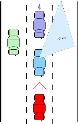
To introduce POMDPs let us consider an example based on the work of McCallum [1996], where an agent learns to drive a car in New York. The agent can look forward, backward, left or right. It cannot change speed but it can steer into the lane it is looking at. Observations from the world take multiple forms. One task of the agent is to learn to fuse or ignore different forms as appropriate. Different types of observation in the New York driving scenario include:
• the direction in which the agent’s gaze is directed;
• the closest object in the agent’s gaze;
• whether the object is looming or receding;
• the colour of the object;
gaze
Figure 1.1: The agent is in control of the middle car. The car behind is fast and will not slow down. The car ahead is slower. To avoid a crash the agent must steer right. However, when the agent is gazing to the right, there is no immediate observation that tells it about the impending crash.
To drive safely the agent must steer out of its lane to avoid slow cars ahead and fast cars behind, as depicted in Figure 1.1. This is not easy when the agent has no explicit goals beyond “performing well,” and no knowledge of how the observations might aid performance. There are no explicit training patterns such as “if there is a car ahead and left, steer right.” However, a scalar reward at each time step is provided to the agent as a performance indicator. The agent is penalised for colliding with other cars or the road shoulder. The only goal hard-wired into the agent is that it must maximise a long-term measure of the rewards.
Two significant problems make it difficult to learn under these conditions. The first is solving the temporal credit assignment problem. If our agent hits another car and is consequently penalised, how does the agent reason about which sequence of actions should not be repeated, and in which circumstances? For example, it cannot assume that the last action: “change lane,” was solely responsible because the agent must change lanes in some circumstances.
immediate sensory impetus for the lane change. Alternatively, if the agent hasmemory then it builds up knowledge of thestate of the world around it and it remembers that it needs to make the lane change.
Partial observability takes two forms: absence of important state information in observations and extraneous information in observations. The agent must use memory to compensate for the former, and learn to ignore the latter. For our car driving agent the colour of the object in its gaze is extraneous (unless red cars really do go faster)
If the agent has access to the complete state — such as a chess playing machine that can view the entire board — it can choose optimal actions without memory. This is possible because of the Markov property which guarantees that the future state of the world is simply a function of the current state and action.
This driving example is non-trivial yet easily breaks down into the simple compo-nents of a POMDP:
• world state: the position and speed of the agent’s car and all other cars;
• observations: hearing a horn honk or observing a slow car ahead;
• memory (agent state): remembering out-of-gaze car locations;
• actions: shifting gaze and steering;
• rewards: penalties for collisions.
To emphasise the generality of the POMDP model, consider the following real-life learning problems in a POMDP framework:
• Learning to walk. Babies learn to walk by observing other people do it, imi-tating them, and being rewarded by the attention of their parents or their ability to reach up to the chocolate cake on the kitchen bench.
• Learning to understand speech. Babies learn to understand the sounds they hear and respond in kind. Temporal credit assignment is hard. For example, it is difficult to associate being chastised with the action of stealing the chocolate cake half-an-hour before. These abstract examples can be made more concrete by considering how to teach robots to walk and understand human speech.
observable through a high failure rate at quality check points. The instantaneous reward is the yield of the plant during the last time period.
The generality of POMDPs makes the learning problem inherently difficult. Markov Decision Processes (MDPs) and early POMDP methods made assumptions that sim-plified the problem dramatically. For example, MDPs assume the state of the world is known (full observability), or that the dynamics of the world are completely known. As algorithms have become more sophisticated, and computers faster, the number of simplifying assumptions have been reduced.
However, the problem of finding the optimal policy given partial observability is PSPACE-hard [Cassandra, 1998], with exact algorithms running in exponential time and polynomial space in the number of state variables and observations. This motivates the use of three of the approximations applied in this thesis: a fixed number of bits of memory, the use of function approximators for controlling memory and actions, and local optimisation.
Because POMDP algorithms learn from rewards they are sometimes collectively referred to as reinforcement learning. Provided the reward signal is constructed care-fully, agents will not be biased toward a particular way of achieving the goal; they can learn concepts that their programmers had never thought of. POMDP methods therefore have great potential in domains where human understanding is incomplete or vague. Examples include learning to play games [Tesauro, 1994, Baxter et al., 2001b], network routing [Tao et al., 2001], call admission control [Baxter et al., 2001a], simulat-ing learnsimulat-ing in the brain [Barlett and Baxter, 1999], medical diagnosis and treatment [Smallwood et al., 1971], and moving target tracking [Pollock, 1970]. In Chapter 10 we will examine speech recognition as a difficult and novel application of POMDPs.
On the other hand, supervised machine learning methods such as error back prop-agation only learn concepts embedded in training patterns: they are only as good as their teacher. Tesuro [1990] trained the NeuroGammon system using previously played games as training examples. This system reached a high intermediate level. The use of explicitly supervised learning limited NeuroGammon to tactics captured by the training examples, ensuring it never developed original and superior tactics. The next attempt was TD-Gammon [Tesauro, 1994] which used reinforcement learning. This resulted in a world champion backgammon machine.
1.1.2 Our Approach
where information can only be gathered through interacting with the world and where memory is required to perform well. The algorithms all share three features:
1. Finite state controllers for agent memory. The agent has a finite set of memory states, or internal states. When the agent receives an observation it can make a transition from one internal-state to another. During training the agent learns to control these transitions so that the internal states provide useful information about past observations and actions. Key advantages of this method over others are:
• the ability to remember key events indefinitely; • the ability to ignore irrelevant events;
• per-step complexity that is at worst quadratic in the number of world states, actions, observations, and internal states.
2. Gradient ascent of the long-term average reward. The agent’s behaviour depends on a set of internal parameters. Our goal is to adjust these parameters to maximise the long-term average reward. We do this by estimating the gradient of the long-term average reward with respect to the agent parameters. Some parameters control the internal-state transitions, and others control the actions the agent chooses at each time step. Key advantages of this method are:
• convergence to at least a local maximum is assured under mild conditions; • the agent learns to choose correct actions without the complex intermediate
step of learning the value of each action;
• system memory usage that is proportional to the number of internal param-eters rather than the complexity of the POMDP.
Potential disadvantages of gradient ascent methods include:
• many trials or simulations of the scenario may be needed to achieve conver-gence;
• we cannot usually guarantee convergence to the global maximum.
The first disadvantage arises from problems such as high-variance in the gradient estimates. This thesis looks at several methods to reduce the number of trials needed. The second disadvantage is typical of local optimisation and we accept this approximation to reduce the algorithmic complexity.
bounds the implications of actions on the reward, (2) introduce an “effective horizon” that is tuned to the problem. The first solution corresponds to the finite-horizon assumption, essentially saying that the POMDP is guaranteed to reset itself periodically. The second solution is the infinite-horizon setting, which is more general because it does not require that anobservablerecurrent state can be identified, or even that one exists. The recurrent state must be observable so that the agent can reset its credit assignment mechanism when the state is encountered. Even when observable recurrent states can be identified, they may occur so infrequently that algorithms that use the finite-horizon assumption may perform poorly.
Effective horizons can be introduced by assuming the reward received was in response to a “recent” action. Alternatively, higher order filters can encode in-formation about the credit assignment problem. The most common approach is to assume that rewards are exponentially more likely to be due to recent actions. Effective horizons satisfy our intuition that we can learn to act well by observing a short window of the overall task. Consider learning to play a card game at a casino. The game may go on indefinitely but a few hands are sufficient to teach someone the basics of the game. Many hands give a player sufficient experience to start to reasoning about long-term strategy.
Chapter 2 will review alternative approaches to implementing memory and training agents.
1.2
Thesis Contributions
This section summarises the contributions of the thesis, simultaneously outlining the rest of the document. Chapter 2 provides a formal introduction to partially observable Markov decision processes, describing historical approaches and placing our work in context. Chapter 3 states some mild assumptions required for convergence of stochas-tic gradient ascent and describes how they can be satisfied. Chapters 4 to 6 introduce our novel policy-gradient algorithms. Chapters 7 and 8 provide some practical im-plementation details and experimental comparisons. The remaining three chapters are largely independent, presenting variance reduction methods, applications of our policy-gradient methods to speech recognition, and fast training using the “Bunyip” Beowulf cluster. The research contributions of each chapter are:
• Chapter 4:
uses a series matrix expansion of the expression for the exact gradient. The algorithm works in the infinite-horizon case, uses finite state controllers for memory, and does not need to gather experience through world interactions. The algorithm takes advantage of sparse POMDP structures to scale to tens-of-thousands of states.
– UsingGAMPwe demonstrate that a noisy multi-agent POMDP with 21,632 states can be solved in less than 30 minutes on a modern desktop computer.
• Chapter 5:
– This chapter introduces IState-GPOMDP, an algorithm that approximates the gradient when a model of the world isnot available. In this case learning can only proceed by interacting with the world. It scales to uncountable state and action spaces and operates in an infinite-horizon setting. This is in contrast to similar previous algorithms that are restricted to finite-horizon tasks. The complexity of each step does not depend on the size of the state space and is linear in the number of internal states.
• Chapter 6:
– The IOHMM-GPOMDP algorithm uses hidden Markov models (HMMs) to estimate the state hidden by partial observability. Existing methods that use HMMs ignore the most useful indicator of performance: the reward.
IOHMM-GPOMDPlearns to predict rewards, thus revealing the hidden state that is relevant to predicting the long-term average reward.
– IState-GPOMDPgathers experience using a single trajectory through world states and internal states. Exp-GPOMDPis an alternative that still samples world states but takes the expectation over all internal-state trajectories. This reduces the variance of gradient estimates at the cost of making the per step complexity quadratic in the number of internal states.
• Chapter 7:
• Chapter 8:
– We present empirical results on a variety of POMDPs, some larger than previous FSC results in the literature, demonstrating the use of sparse FSC methods on difficult scenarios.
• Chapter 9:
– We introduce two novel methods that reduce the variance of gradient es-timates. The first details how to estimate gradients using infinite impulse response filters to encode domain knowledge. The second proposes learning a subset of the parameters with value-function methods to take advantage of their relatively low variance.
– The application of an existing variance reduction method to our gradient estimates is described. This method uses a fixed sequence of random num-bers to perform Monte-Carlo estimates. Our investigation shows that this method must be used with care because it can introduce a form of over-fitting.
• Chapter 10:
– We investigate the use of our algorithms on a large-scale, difficult, real-world problem: speech recognition. We list some advantages of POMDP models over existing speech frameworks. A series of experiments are conducted starting with the simple problem of discriminating binary sequences, moving onto discriminating between spoken digits, and ending with a foray into large vocabulary connected speech recognition (LVCSR). We demonstrate results that are competitive with methods using similar models but trained traditionally.
• Chapter 11:
– The scale of problems such as LVCSR requires the use of super-computing time. Our small budget demanded ingenuity in constructing a cost-effective super-computer. We outline the hardware and software behind the team effort that won a Gordon-Bell prize in 2001, creating the world’s first sub USD $1 per MFlop/s super-computer: the “Bunyip” Beowulf-cluster. This cluster was used for many of the experiments in this thesis.
1.3
Notation
This section describes notation conventions and shortcuts used throughout the thesis. Calligraphic letters refer to a set and an element of that set is represented by the corresponding lowercase letter. A concession to convention is the set of states S with elements represented byi∈ S. When two elements of the same set are referred to, the second element uses the next letter in the alphabet, or a time subscript, to distinguish them. For example, g ∈ G, h ∈ G or gt ∈ G, gt+1 ∈ G. Summations over multiple sets will often just use the subscripts to indicate which sets the summation is over, for example,
X
i,g
means X
i∈S X
g∈G
.
Functions of the form µ(u|θ, h, y) should be understood as the probability of event u ∈ U as a function of the variables to the right of the ‘|’. If one of the variables is omitted we mean that the probability ofuis independent of that variable, for example, µ(u|θ, y) means h plays no part in evaluating the probability of u in the context of the surrounding material. The quantities θ ∈ Rnθ and φ ∈ Rnφ represent vectors of adjustable parameters.
Much of this work is concerned with state transitions and trajectories of states. The former will usually be discussed with consecutive alphabetic letters, for example, a transition from state i to state j. When talking about trajectories we use the first letter and time subscripts, for example, a transition from state it to state it+1. Thus
ω(h|φ, g, y) means the same thing as ω(gt+1|φ, gt, yt) except the former could be any
transition in the trajectory and the latter is the transition at time t.
Uppercase letters always refer to matrices. Lowercase letters can refer to scalars or column vectors. Subscripts generally refer to a value at time t, for example, it means
the value ofiat time t. When referring to the value of thei’th element of the vectora at timet we use the notationat(i). Occasional exceptions to any of these conventions
Existing POMDP Methods
Oh yes, and don’t forget the other important rule of CS dissertations construction: always include a quote from Lewis Carroll.
—Spencer Rugaber
In this chapter we introduce our view of agents interacting with the world. Past approaches are discussed and we motivate our use of finite-memory policy-gradient methods as a means of training agents. The chapter covers a broad range of algorithms, forming a snapshot of research into POMDPs.
After formalising the framework that we will use throughout this thesis, Section 2.5 discusses exact and approximate methods for solving POMDPs when the underlying POMDP parameters are known. Section 2.6 discusses methods that assume these parameters are not known. This thesis describes novel algorithms for both settings. Section 2.7 describes miscellaneous methods for variance reduction and multi-agent settings.
2.1
Modelling the World as a POMDP
Our setting is that of an agent taking actions in a world according to its policy. The agent receives feedback about its performance through a scalar reward rt received at
each time step.
Definition 1. Formally, a POMDP consists of:
• |S| states S ={1, . . . ,|S|} of the world;
• |U| actions (or controls) U ={1, . . . ,|U|} available to the policy;
• |Y| observations Y ={1, . . . ,|Y|};
• a (possibly stochastic) reward r(i)∈Rfor each state i∈ S.
Agent
POMDP
MDPPartial Observability
world−
state
ν(yt|it) it
r(it+1)
it+1
yt
rt+1
[image:28.595.158.391.107.326.2]ut q(it+1|it, u)
Figure 2.1: Diagram of the world perspective of POMDP showing the underlying MDP, and the stochastic process ν(yt|it) mapping the current state it to an observation yt, thus hiding
the true state information.
algorithms. Baxter and Bartlett [2001] provide a convergence proof for uncountable state and action spaces for the algorithm that is the parent of those in this thesis.
Each action u ∈ U determines a stochastic matrix [q(j|i, u)]i=1...|S|,j=1...|S|, where
q(j|i, u) denotes the probability of making a transition from state i∈ S to state j∈ S given action u∈ U. For each state i, an observationy∈ Y is generated independently with probabilityν(y|i). The distributions q(j|i, u) andν(y|i), along with a description of the rewards, constitutes the model of the POMDP shown in Figure 2.1.
Conceptually, the world issues rewards after each state transition. Rewards may de-pend on the action and the previous statert+1=r(it, ut); but without loss of generality
we will assume rewards are a function of only the updated state rt+1 =r(j) =r(it+1)
so that r1 is the first reward, received after the first action.1
If the state is not hidden, that is, there is an observation y for each world state and ν(y|i) = 1 if y = i, then we are in the MDP setting. This setting is significantly easier than the POMDP setting with algorithms running in time that is O(|S|2) per iteration, or O(|S|3) for a closed form solution [Bellman, 1957]. MDP research was the precursor to the study of POMDPs so in Section 2.4 we briefly mention some of the most influential MDP algorithms. POMDPs may beepisodic, where the task ends upon the agent entering a state i∗ which is in the set of termination states S∗ ⊂ S.
1The more general case can be obtained by augmenting the state with information about the last
r = 1 0 0 0 0 1
U N N N N L
(a)
Left Right
L U
U L
NULL NULL
(b)
Figure 2.2: 2.2(a) The Load/Unload scenario with 6 locations. The agent receives a reward of 1 each time it passes through the unload location U, or the load locationL, after having first passed through the opposite end of the road. In each state the agent has a choice of two actions: either leftor right. The three observations are Y ={U, N, L}, which are issued in the unloading state, the intermediate states and the loading states respectively. 2.2(b) The policy graph learned for the Load/Unload scenario. Each node represents an internal state. The “Left” state is interpreted as: I have a load so move left, and the “Right” state as: I dropped my load so move right. The dashed transitions are used during learning but not by the final policy.
More generally, they may be infinite-horizon POMDPs that conceptually run forever.
2.2
Agents with Internal State
We have already asserted that agents generally require internal state, or memory, to act well. To make this concept concrete, consider the Load/Unload scenario [Peshkin et al., 1999] shown in Figure 2.2(a). The observations alone do not allow the agent to determine if it should move left or right while it occupies the intermediateNobservation states. However, if the agent remembers whether it last visited the load or unload location (1 bit of memory) then it can act optimally.
We now introduce a generic internal-state agent model that covers all existing algorithms. We will use it to compare algorithms and introduce our novel algorithms. The agent has access to a set of internal states g ∈ G = {1, . . . ,|G|} (I-states for short). Finite memory algorithms have finite G. Alternatively, exact infinite-horizon algorithms usually assume infiniteG.2 For example, one uncountable form of G is the
2It is an abuse of notation to write g ∈ G = {1, . . . ,|G|} when G could be uncountably infinite,
set of all belief states: distributions over world state occupancy in the |S| dimension simplex. The cross product of the world-state space S and the internal-state space G form the global-state space.
The agent implements a parameterised policy µ that maps observations y ∈ Y, and I-states h ∈ G, into probability distributions over the controls U. We denote the probability underµof controlu, given I-stateh, observationy, and parametersθ∈Rnθ, by µ(u|θ, h, y). Deterministic policies emit distributions that assign probability 1 to action ut and 0 to all other actions. Policies are learnt by searching the space of
parameters θ∈Rnθ.
The I-state evolves as a function of the current observation y ∈ Y, and I-state g ∈ G. Specifically, we assume the existence of a parameterised functionω such that the probability of making a transition to I-state h ∈ G, given current I-state g ∈ G, observation y ∈ Y, and parameters φ ∈ Rnφ, is denoted by ω(h|φ, g, y). The I-state transition function may be learnt by searching the space of parameters φ∈Rnφ.
An important feature of our model is that both the policy and the I-state transitions can be stochastic.
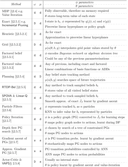
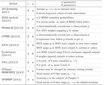
Some algorithms do not learn the I-state transition function, fixing φ in advance. Examples include the exact methods of Section 2.5.1, where we can write down the equations that determine the next belief state from the previous belief state and cur-rent observation. Algorithms that learn the internal-state transitions include the class of methods we use in this thesis, that is, policy-gradient methods for learning finite state controllers. Throughout this section we compare algorithms in terms of how the ω(h|φ, g, y) andµ(u|θ, h, y) functions work and how they are parameterised. Tables 2.1 and 2.2 summarise these differences at the end of the chapter.
The agent’s view of the POMDP is represented by Figure 2.3. The POMDP evolves as follows:
1. let i0 ∈ S and g0 ∈ G denote the initial state of the world and the initial I-state of the agent respectively;
2. at time step t, generate an observationyt ∈ Y with probability ν(yt|it);
3. generate a new I-state gt+1 with probability ω(gt+1|φ, gt, yt);
4. generate actionut with probabilityµ(ut|θ, gt+1, yt);
5. generate a new world stateit+1 with probability q(it+1|it, ut);
I−state
Agent
µ(ut|θ, gt+1, yt)
ω(gt+1|φ, gt, yt)
g
World
rt+1
gt+1
yt ut
ν Q r
Figure 2.3: POMDP from the agent’s point of view. The dashed lines represent the extra information available for model-based algorithms.
2.3
Long-Term Rewards
Our algorithms attempt to locally optimise θ ∈ Rnθ and φ ∈ Rnφ, maximising the long-term average reward:
η(φ, θ, i, g) := lim
T→∞
1 TEφ,θ
" T X
t=0
r(it)|i0 =i, g0 =g #
, (2.1)
where Eφ,θ denotes the expectation over all global trajectories {(i0, g0), . . . ,(iT, gT)}
when the agent is parameterised by φ and θ. An alternative measure of performance is the discounted sum of rewards, introducing a discount factor β ∈[0,1)
Jβ(φ, θ, i, g) :=Eφ,θ
"∞ X
t=0
βtr(it)|i0 =i, g0=g #
. (2.2)
The exponential decay of the impact of past rewards is equivalent to the assumption that actions have exponentially decaying impact on the current performance of the agent as time goes on. Alternatively, this can be viewed as the assumption that rewards are exponentially more likely to be generated by the most recent actions.
Fortu-nately, when the agent is suitablymixing, maximising one is equivalent to maximising the other. Suitably mixing means that η(φ, θ, i, g) is independent of the starting state (i, g) and so may be written η(φ, θ). In other words, the POMDP is ergodic. In this case, there is also a unique stationary distribution over world/internal state pairs. The conditions necessary to ensure ergodicity are mild and will be given in Chapter 3. We denote the expectation over this stationary distribution withEi,g. For ergodic POMDPs
the long-term average reward and the discounted reward are related by [Baxter and Bartlett, 2001]
Ei,gJβ(θ, φ, i, g) =
1
1−βEi,gη(φ, θ, i, g).
2.4
Methods for Solving MDPs
In this section we describe dynamic programming methods that apply when the state is fully observable, that is, the MDP setting. We will restrict ourselves to the discounted reward setting though the methods can often also be applied to average rewards.
If we have a method of determining the long-termvalue of each state then the agent can act by choosing the action that leads to the state with the highest value. The value is the expected discounted reward for entering stateiunder the optimal policy. Bellman [1957] describes a procedure known as dynamic programming (DP) which allows us to determine the value J∗
β(i) for each state i ∈ S. We drop the dependency of Jβ∗(i) on
φ and θ for this section because DP computes the optimal value directly rather than the value gained by a particular agent. The MDP assumption means that memory is not necessary. This is equivalent to having a single internal state, making the memory processω(h|φ, g, y) trivial. Such agents are said to implementreactive policies. DP is described by the Bellman equation, whereβ ∈[0,1) is a discount factor that weights the importance of the instantaneous reward against the long-term reward
Jβ∗(i) = maxu
r(i) +βX
j∈S
q(j|i, u)Jβ∗(j)
. (2.3)
Assuming we can store a value estimate for each state, DP proceeds by replacingJβ∗(i) with an estimate Jβ(i) and iterating
Jβ(i)←max u
r(i) +βX
j∈S
q(j|i, u)Jβ(j)
. (2.4)
[Bert-sekas and Tsitsiklis, 1996]. OnceJ∗
β(i) is known the optimal policy is given by
u∗i = arg maxu
r(i) +βX
j∈S
q(j|i, u)Jβ∗(j) .
To reflect full observability, and the absence of internal state, we write the policy as µ(u|θ, i) instead of µ(u|θ, h, y). For MDPs the optimal µ is deterministic and equal to
µ(u|θ, i) =χu(u∗i), (2.5)
whereχm(k) is the indicator function
χm(k) :=
1 ifk =m,
0 otherwise. (2.6)
Recall that the vectorθparameterises the policy. In the MDP caseθcould represent the value of each state i∈ S or it could represent the mapping of states to actions derived from those values. In the later case θ would be a vector of length |S|, representing a table mapping states directly to the optimal action for that state. When the state and action spaces are large we resort to some form of function approximator to represent the table. For example, the parameters θ could be the weights of an artificial neural network (ANN) that maps states to actions. Function approximation for DP was in use by Bellman et al. [1963] and possibly earlier.
Iterating Equation (2.4) until convergence, and forming a policy from Equation (2.5) is the basis ofvalue iteration [Howard, 1960]. Alternatively, policy iteration [Bellman, 1957] learns the value of states under a particular agent, denoted Jβ,µ(i). Once the
value of the policy has been learnt the policy is updated to maximiseJβ,µ(i), followed
by a re-evaluation ofJβ,µ(i) under the new policy. This is repeated until the policy does
not change during maximisation. Policy iteration resembles Expectation-Maximisation (EM) methods [Dempster et al., 1977] because we estimate the expected value for state i, then alter the policy to maximise the expected value fori.
Evaluating (2.4) has complexity O(|U||S|2) per step which, while polynomial, is infeasible for very large state spaces. Also, the transition probabilities q(j|i, u), which are part of the model, may not always be available. These two observations moti-vate Monte-Carlo methods for computing Jβ∗(i). These methods learn by interacting with the world and gathering experience about the long-term rewards from each state.
γt ∈[0,1)
Q(it, ut)←Q(it, ut) +γt[rt+1+βmax
u0 Q(it+1, u
0)−Q(i
t, ut)],
which states that the value Q(it, ut) should be updated in the direction of the error
[rt+1 +βmaxu0Q(it+1, u0)]−Q(it, ut). The values converge provided an independent
value is stored for each state/action pair, each state is visited infinitely often, and γ is decreased in such a way that Ptγt = ∞ and Ptγt2 < ∞ [Mitchell, 1997].
Q-learningis anoff-policy method, meaning the optimal policy can be learnt by following a fixed alternative policy. This allows a reduction of the number of expensive world interactions by repeatedly re-using experience gathered under an old policy to improve the current policy.
The complexity of learningJβ∗(i) orQ(i, u) can be reduced by automatically aggre-gating states into clusters of states, or meta-states, at the cost of introducing partial observability [Singh et al., 1995, Engel and Mannor, 2001].
Readers interested in MDPs are referred to books such as Puterman [1994], which covers model-based algorithms and many variants on MDPs. Bertsekas and Tsitsik-lis [1996] provides an analysis of the convergence properties of MDP algorithms and Kaelbling et al. [1996] describes the algorithms from the reinforcement learning point of view.
2.5
Learning with a Model
This section describes existing methods for producing POMDP agents when the model of the POMDP is known, which is equivalent to knowing ν(y|i), q(j|i, u) and r(i). These include exact methods that are guaranteed to learn the optimal policy given sufficient, possibly infinite, time and memory. We define the optimal agent as the agent that obtains the maximum possible long-term (average or discounted) reward given that the agent does not have access to the true state of the system. The long-term reward of optimal MDP methods upper bounds the reward that can be obtained after introducing partial observability [Hauskrecht, 2000].
2.5.1 Exact Methods
The observation process may not reveal sufficient state to allow reactive policies to choose the optimal action. One solution is to model an agent that remembers its entire observation/action history ¯y. This fits within our framework by setting G to be the sequence of all past observations and actions ¯y ={(y0, u0), . . . ,(yt, ut)}. Using
¯
if ¯y does not allow the agent to determine the true state, it may help to reduce the entropy of the agent’s belief of which state it occupies, consequently improving the probability that the agent will act correctly. In this case G is the possibly infinite set of all observation/action trajectories and ω(h|φ, g, y) is a deterministic function that simply concatenates the last observed (yt, ut) to ¯y.
Consider an agent in a symmetric building. If it only receives observations about what is in its line of sight, then many places in the building will appear identical. However, if it remembers the last time it saw a landmark, such as the front doors of the building, then it can infer where it is in the building from its memory of how it moved since seeing the landmark. This is the approach taken by methods such as utile distinction trees [McCallum, 1996] and prediction suffix trees [Ron et al., 1994]. These methods do not necessarily assume knowledge of the POMDP model and will be discussed in Section 2.6.
2.5.1.1 Belief States
Explicitly storing ¯y results in inefficient memory use because we potentially need to store an infinite amount of history in infinite-horizon settings. ˚Astr¨om [1965] described an alternative to storing histories which is to track the belief state: the probability distribution over world-states, S, given the observation and action history ¯y. The belief state is a sufficient statistic in the sense that the agent can perform as well as if it had access to ¯y [Smallwood and Sondik, 1973]. We use the notationbt(i|¯yt) to mean
the probability that the world is in state i at time t given the history up to time t. Given a belief state bt, an action ut, and an observationyt, the successor belief state is
computed using
bt+1(j|y¯t) =
ν(yt|j)Pi∈Sbt(i|y¯t)q(j|i, ut)
P
y0∈Yν(y0|j)Pi∈Sbt(i|¯yt)q(j|i, ut)
. (2.7)
In this setting G is the possibly uncountable set of belief states the system can reach. From this point on we will useBinstead ofGto refer to the set of reachable belief states, allowing us to keep the belief state distinct from other forms of internal state such as finite state controller I-states. Each element b ∈ B is a vector in an |S| dimensional simplex. The function ω(bt+1|φ, bt, y) is deterministic, giving probability 1 to vector
bt+1 defined by Equation (2.7).
1973, Cassandra et al., 1994]
¯
Jβ(b0)←max u
" ¯
r(b0) +βX
b∈B
¯
q(b|b0, u) ¯Jβ(b)
#
, (2.8)
which converges in finite time to within of the optimal policy value [Lovejoy, 1991]. The bar on ¯Jβ(b) indicates that we are learning values of belief states b instead of
world states i. The simplicity of this equation is misleading because ¯Jβ, ¯r, and ¯q
are represented in terms of their MDP counterparts in Equation (2.3). For example, ¯
r(b) = Pi∈Sbir(i). When the set of reachable belief states can be infinite, ¯Jβ(b) is
significantly more complex than Jβ(i), which is the subject of the next section.
2.5.1.2 Value Function Representation
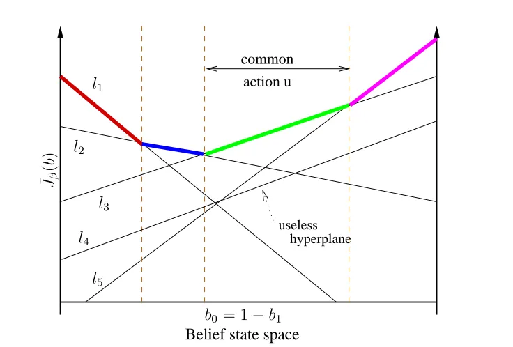
Maintaining and updating independent values for infinitely many belief states is infea-sible. Fortunately, it has been shown for finite horizons that the value over all belief states can be represented exactly by a convex piecewise linear function [Smallwood and Sondik, 1973]. Such a representation is shown for a 2 state system in Figure 2.4. The set L contains the hyperplanes needed to represent the value function. Each l∈ L is an |S| dimensional vector such that the value of hyperplanel for belief state b is b·l. The value of ¯Jβ(b) is the maximum over all hyperplanes
¯
Jβ(b) = max l∈L{b·l}.
To be useful, a hyperplane l must be the maximum for some b. If L contains only useful hyperplanes then it is called aparsimonious set [Zhang, 1995].
Estimating the value function proceeds by using value iteration on belief states chosen to be points in the belief simplex that have a unique maximuml l, and that have not yet converged to their true value. These points, as found by the Witness
algorithm, are called witness points [Cassandra et al., 1994]. This term is now often used to describe any belief state upon which it is useful to perform a DP update. Such updates generate new vectors to be added to L. A difficult task — and the way in which most exact POMDP algorithms differ — is determining the witness points efficiently. This is often done by solving a set of linear programs. Once a single round of value iteration has been performedLis examined to remove useless vectors, creating a parsimonious set ready for the next round.
common action u
Belief state space
useless hyperplane
l1
l2
l3
l5
l4 ¯J(β
b
)
[image:37.595.144.512.96.345.2]b0 = 1−b1
Figure 2.4: Convex piecewise linear representation of a value function for a continuous belief state with|S|= 2. The plot is a slice from a 3-dimensional plot defined by valid points in the the 2-dimensional simplex, that is, whereb0= 1−b1. If the setLis parsimonious then eachln
defines a line segment which is maximum in some partition of belief space. Each such partition has a unique optimal actionu∗
n.
sophistication other algorithms include the One-Pass algorithm of Sondik [1971], the
Linear Support algorithm of Cheng [1988], the Witness algorithm of Cassandra et al. [1994], and the Incremental Pruning algorithm of Zhang and Liu [1996]. Cassandra [1999] provides a non-mathematical comparison of these algorithms.
2.5.1.3 Policy Representation
POMDP agents can be represented by a policy graph that is a directed and possibly cyclic graph. Each node is labelled with a single action and transitions out of each node are labelled with observations. All nodes map to a polyhedral partition in the value function. Partitions are defined by the region where a single hyperplane l ∈ L maximises ¯Jβ(b) [Cassandra et al., 1994]. Transitions between nodes in the policy graph
are a deterministic function of the current observation. Actions are a deterministic function of the current node. If the optimal policy can be represented by a cyclic graph with a finite number of nodes, then the POMDP is called finitely transient [Sondik, 1978].
to the action associated with the hyperplane that maximises the value at bt. If the
policy is finitely transient it can be represented more compactly by the policy graph. In this case the internal statesG are equivalent to the policy-graph nodes. The I-state (internal state) update ω(h|φ, g, y) uses y to index the correct transition from node g to node h. The policy µ(u|θ, h) is simply a lookup table that gives the optimal action for each nodeh. Thus,φrepresents policy-graph transitions, andθmaps policy-graph nodes to actions.
In many cases it is possible for large infinite-horizon POMDPs to be controlled well by simple policy graphs. Consider the Load/Unload scenario [Peshkin et al., 1999] shown in Figure 2.2(a). The optimal policy graph is shown in Figure 2.2(b). This policy graph suffices no matter how many intermediate locations there are between the load and unload locations. As the number of intermediate locations increases, the value function becomes more complex but the optimal policy graph does not. This example partially motivates the idea (discussed in Section 2.5.7) of searching in the space of policy graphs instead of learning value functions.
2.5.1.4 Complexity of Exact Methods
There are two problems with exact methods that make them intractable for problems with more than a few tens of states, observations, and actions. To discuss the first we introduce the concept of state-variables. State variables describe the state in terms of features that are true or false, which is an arguably more intuitive description than enumerating states. Consider a system with v boolean state variables. The number of POMDP states is |S| = 2v, thus |S| grows exponentially with the number of state
variables. For example, two state variables might be “is it raining?” and “is the umbrella open?” requiring 4 states to encode.
Since DP for POMDPs involves updating belief states, the complexity of POMDP algorithms grows exponentially with the number of state variables. This makes belief-state monitoring infeasible for large problems [Boyen and Koller, 1998, Sallans, 2000]. The second problem is representing ¯Jt(b), the value function after t steps of DP.
LetBt be the set of belief states reachable at time t. Recall that |Y| is the number of
possible observations. Assuming |B0| = 1, that is, a single known initial belief state, then after tsteps of a greedy policy we potentially have|Y|t belief states inB
t. Thus,
the problem of representing ¯Jβ(b) grows exponentially in the horizon length. Since
the belief-state space is infinite for infinite horizons, exact methods perform DP on the hyperplanes in L. This representation grows exponentially in the observations since a single DP step in the worst case results in|Lt+1|=|U||Lt||Y|[Cassandra, 1998].
requires solving expensive linear programs.
Even for simplified finite-horizon POMDPs, the problem of finding the optimal policy is PSPACE-hard [Papadimitriou and Tsitsiklis, 1987]. Learning a policy graph with a constrained number of nodes is NP-hard [Meuleau et al., 1999a]. Infinite-horizon POMDPs can result in an infinite number of belief states or hyperplanes l, resulting in the problem of determining convergence being undecidable [Madani et al., 1999]. Even worse, determining -convergence is undecidable in polynomial time for finite-horizon POMDPs [Lusena et al., 2001]. Despite this gloomy theoretical message, empirical results, such as those in this thesis, show that it is possible to learn reasonable policies in reasonable time for POMDPs of ever increasing complexity. We avoid the intractable computational complexity of exact methods by abandoning the requirement that policies be optimal, while retaining the requirement that agents should at least converge to a fixed policy.
2.5.2 Approximate Value Function Methods
This section introduces model-based methods that learn approximations to Jβ∗(i). For a more detailed survey of these methods see Hauskrecht [2000].
2.5.2.1 Heuristics for Exact Methods
A number of methods simplify the representation of ¯Jβ(b) by assuming the system
is an MDP and learning the underlying Q-function Q(i, u). This must be done via model-based methods or by computer simulation because the partial observability of the real world does not allow ito be known during real-world interaction.
One choice for the policy is [Nourbakhsh et al., 1995]
¯
u∗(b) = arg max
u Q(arg maxj b(j), u), µ(u|θ, b) =χu(¯u
∗(b)),
which assumes the agent is in the most likely state (MLS), known as the MLS heuristic. This approach completely ignores the agent’s confusion about which state it is in. The voting heuristic [Simmons and Koenig, 1995] weights the vote for the best action in each state by the probability of being in that state
u∗(j) = arg max
a Q(j, a), ¯u
∗(b) = arg max
u
X
j∈S
b(j)χu(u∗(j))Q(j, u∗(j)).
for one step and then assumes that the state is entirely known [Cassandra, 1998]
¯
u∗(b) = arg max
u
X
j∈S
b(j)Q(j, u).
These heuristics will perform poorly if the belief state is close to uniform. Due to the convexity of the value function, ¯Jβ(b) generally grows as the entropy ofbdecreases.
The highest expected payoffs occur at the simplex corners. This motivates choosing actions that decrease the entropy of the belief state in the hope that the heuristics above will perform better with a peaked belief. For example, consider a robot that must reach the other side of a featureless desert [Roy and Thrun, 2001]. If it goes straight across it will quickly become lost due to lack of landmarks and movement errors. The better policy is to skirt the desert, taking longer but remaining certain of reaching the goal because the robot is certain of its location. Cassandra [1998] shows how to use the entropy of b to switch between information gathering policies and exploitive policies. The entropy can also be used to weight two policies that trade off information gathering and exploitation. These heuristics may be misleading if the minimum of ¯Jβ(b) does not occur at the point of greatest entropy, that is, the uniform
belief state.
An alternative family of heuristics are based on simplified versions of the full DP update. For example, determining maximising vectors inLfor each state, rather than over all states, produces the fast informed bound of Hauskrecht [1997]. The heuristics in this section are also useful as upper bounds on Jβ∗, allowing them to direct tree search procedures used in classical planning approaches (see Section 2.5.4).
2.5.2.2 Grid Methods
Value functions over a continuous belief space can be approximated by values at a finite set of points along with an interpolation rule. Once a set of grid points has been chosen an equivalent MDP can be constructed where the states are the grid points. This POMDP can be solved in polynomial time [Hauskrecht, 2000]. The idea is equivalent to constructing a policy graph where each node is chosen heuristically to represent what might be an “interesting” region of belief state space. The two significant issues are how to choose grid points and how to perform interpolation.
[Brafman, 1997].3
Interpolation schemes should maintain the convex nature of the value function and hence are typically of the form
¯
Jβ(b) = arg max u
X
g∈G
λg,bf(g, u), (2.9)
where Pg∈Gλg,b = 1 and λg,b ≥ 0 ∀g, b. The function f(g, u) represents the value
grid pointg under actionu. Examples include nearest neighbour, linear interpolation, and kernel regression [Hauskrecht, 2000]. The MLS heuristic can be thought of as a grid method with points at the belief-simplex corners and a simple 1-nearest-neighbour interpolation (assuming anL∞ distance measure) [Brafman, 1997].
Recently, -convergence was shown for a grid method by using -covers under a specifically chosen distance metric [Bonet, 2002]. Within our knowledge it is the only provably optimal grid based algorithm. It is still intractable because the number of grid points required grows exponentially with the size of the state space.
Alternatively, grid point value estimation steps can be interleaved with exact hy-perplane DP updates in order to speed up DP convergence without sacrificing policy optimality [Zhang and Zhang, 2001].
In the context of grid methods the ω(bt+1|φ, bt, yt) process still performs a
deter-ministic update on the belief state, but now µ(u|θ, bt+1, yt) represents the choice of
action based on the interpolated value from (2.9). The θ parameters store the values of actions at the grid points.
2.5.3 Factored Belief States
Using the state variable description of a POMDP (discussed in Section 2.5.1.4) is some-times referred to as belief factorisation, especially when the factorisation is not exact. The value of a state variableXt may depend (approximately) on a small subset of the
state variables at the previous time steps. Transition probabilities can be represented by a two-slice temporal Bayes net (BN) that models the dependencies between state variables over successive time steps as a 2 layer acyclic graph [Dean and Kanazawa, 1989] (see Figure 2.5). Each node contains a conditional probability table showing how its parents affect the probability of the state variable being true.
Alternatively, the state variable dependencies can be represented by a tree structure such as analgebraic decision diagrams (ADD) [Bahar et al., 1993]. BNs and ADDs are applied to POMDPs by Boutilier and Poole [1996] to simplify both the belief monitoring
3The mutual observations requirement is an interesting heuristic that may identify whether belief
Z
X’
X Y
Z’ Y’
Figure 2.5: Two-slice temporal Bayes network showing dependencies between state variables over successive time steps. X andZdepend only on themselves butY is influenced by itself and
X. This conditional dependence structure can be exploited to efficiently model the transition probabilities of a POMDP.
problem and the value function representation problem. We now describe how recent work has used belief factorisation to solve each of these problems.
2.5.3.1 Efficiently Monitoring Belief States
Boyen and Koller [1998] observed that representing belief states as BNs can lead to an accumulation of errors over many time steps that result in the belief state approxi-mation diverging. The authors show that projections of the BN that produce strictly independent groups of state variables results in converging belief-states, allowing re-covery from errors. These projections can be searched to automatically determine BNs that perform well under a specified reward criterion. Heuristic methods to determine factorisations were introduced by Poupart and Boutilier [2000]. These were improved in Poupart and Boutilier [2001] which presents a vector-space analysis of belief-state approximation, providing a formally motivated search procedure for determining belief-state projections with bounded errors. This expensive off-line calculation speeds up on-line belief state tracking.
An alternative method of searching for the optimal belief factorisation is to learn a dynamic sigmoid belief network [Sallans, 2000]. Stochastic gradient ascent is performed in the space of BNs with a fixed number of dependencies, minimising the error between the belief state and the approximation. This algorithm has been applied to the large New York driving problem of McCallum [1996] which was sketched out in Section 1.1. Unlike the algorithms considered so far, which apply a fixed I-state update through ω(h|φ, g, y), this algorithm can be viewed as learningω(h|φ, g, y) by adjusting the belief network parameterised byφ.
2.5.3.2 Factored Value Functions
the transition model are found, they may not induce a similar structure on the value function. The same paper discusses factored value functions implemented as weighted linear combinations of polynomial basis functions. The weights are chosen to minimise the squared error from the true value. In our model of agents the weights would be represented by θ.
This idea is combined with BNs for belief monitoring by Guestrin et al. [2001a]. With approximate belief monitoring and factored linear value functions, DP methods become more feasible since learning reduces to solving systems of linear equations instead of a linear program for every vector inL. The empirical advantages of factored value functions are studied in [Hansen and Feng, 2000] which uses algebraic decision diagrams to represent ¯Jβ(b).
2.5.4 Classical Planning
The link between classical planning algorithms such as C-Buridan[Draper et al., 1994] and POMDP algorithms is summarised by Blythe [1999]. One planning approach is to search the tree of possible future histories ¯y to find the root action with the highest expected payoff. Branch and bound approaches such as the AO∗ algorithm [Nilsson,
1980, §3.2] can be used, searching the tree to a finite depth and pruning the search by eliminating branches that have upper bounds below the best current lower bound. At the leaves the upper and lower bounds can be estimated using QM DP and the
value-minimising-action respectively [Washington, 1997].
This idea is applied to factored finite-horizon POMDPs by McAllester and Singh [1999]. While avoiding the piecewise linear value function, the algorithm is still ex-ponential in the horizon due to the tree search procedure. Furthermore, since there is no concise policy representation the exponential complexity step is performed dur-ing normal policy execution instead of only durdur-ing a learndur-ing phase. In this case ω(bt+1|φ, bt, yt) is responsible for deterministically tracking the factored belief state,
and µ(u|θ, b) is responsible for performing the tree search in order to find the best u. The parametersθare not learnt, butφcould be learnt to optimise factored belief state tracking, as in Section 2.5.3.1.
2.5.5 Simulation and Belief States
an iteration of (2.8) for the current point in belief state space instead of the associated l∈ L[Geffner and Bonet, 1998]. This algorithm, calledRTDP-Bel, does not address the problem of representing Q(b, u) for many belief states over large horizons. However, it has been applied to solving finite-horizon POMDPs with hundreds of states and long-term memory. In particular, it has been applied to the Heaven/Hell scenario that we shall investigate in Chapter 8.
Usually we need to learnQ-functions that generalise to all b. A simple approach is
Linear-Qwhich definesQ(b, u) =φu·b[Littman et al., 1995]. This method is equivalent
to training a linear controller using stochastic gradient ascent with training patterns given by inputs bt and target outputs r+βmaxuQ(bt+1, u). The SPOVA algorithm
[Parr and Russell, 1995] is essentially the same scheme, using simulation to generate gradients for updating the smooth approximate function
¯ Jβ(b) =
" X
l∈L
(b·l)k #1
k ,
wherek is a tunable smoothing parameter and the number of hyperplanes|L| is fixed. Artificial neural networks (ANNs) can also be used to approximate value functions with either the full belief state or a factored representation used as the input [Rodr´ıguez et al., 2000]. Both Linear-Qand SPOVAlearn theθ parameters but notφ.
2.5.6 Continuous State and Action Spaces
Thrun [2000] extends value iteration for belief states into continuous state spaces and action spaces. Since infinite memory would be needed to exactly represent belief states, Thrun uses a sampled representation of belief states. The algorithm balances accuracy with running time by altering the number of samples n used to track the belief state. The belief state is updated using a particle filter [Fearnhead, 1998] that converges to the true belief state as n → ∞, for arbitrary continuous distributions q(j|i, u) and ν(y|i). Approximate continuous belief states are formed from the samples using Gaus-sian kernels. The hyperplane value-function representation cannot be used because the belief state is a continuous distribution, equivalent to infinitely many belief state dimensions. Even function approximators like neural networks cannot trivially con-tend with continuous belief states. Instead, the value function is approximated using a nearest neighbour method where the output value is the average of the k nearest neighbours (KNN) of previously evaluated infinite-dimension belief states.