Identification of the time-dependent conductivity of an inhomogeneous diffusive material

This is a repository copy of Identification of the time-dependent conductivity of an inhomogeneous diffusive material.

White Rose Research Online URL for this paper: http://eprints.whiterose.ac.uk/88367/

Version: Accepted Version

Article:

Hussein, MS and Lesnic, D (2015) Identification of the time-dependent conductivity of an inhomogeneous diffusive material. Applied Mathematics and Computation, 269. 35 - 58. ISSN 0096-3003

https://doi.org/10.1016/j.amc.2015.07.039

© 2015, Elsevier. Licensed under the Creative Commons Attribution-NonCommercial-NoDerivatives 4.0 International http://creativecommons.org/licenses/by-nc-nd/4.0/

[email protected] https://eprints.whiterose.ac.uk/

Reuse

Unless indicated otherwise, fulltext items are protected by copyright with all rights reserved. The copyright exception in section 29 of the Copyright, Designs and Patents Act 1988 allows the making of a single copy solely for the purpose of non-commercial research or private study within the limits of fair dealing. The publisher or other rights-holder may allow further reproduction and re-use of this version - refer to the White Rose Research Online record for this item. Where records identify the publisher as the copyright holder, users can verify any specific terms of use on the publisher’s website.

Takedown

If you consider content in White Rose Research Online to be in breach of UK law, please notify us by

Identification of the Time-Dependent Conductivity of

an Inhomogeneous Diffusive Material

M.S. Hussein1,2 _{and D. Lesnic}1

1_{Department of Applied Mathematics, University of Leeds, Leeds LS2 9JT, UK}

2_{Department of Mathematics, College of Science, University of Baghdad, Baghdad, Iraq}

E-mails: [email protected] (M.S. Hussein), [email protected] (D. Lesnic).

Abstract

In this paper, we consider a couple of inverse problems of determining the time-dependent thermal/hydraulic conductivity from Cauchy data in the one-dimensional heat/diffusion equation with space-dependent heat capacity/ specific storage. The well-posedness of these inverse problems in suitable spaces of continuously differentiable functions are stud-ied. For the numerical realisation, the problems are discretised using the finite-difference method and recast as nonlinear least-squares minimization problems with a simple posi-tivity lower bound on the unknown thermal/ hydraulic conducposi-tivity. Numerically, this is effectively solved using thelsqnonlinroutine from the MATLAB toolbox. Regularization is included wherever necessary. Numerical results are presented and discussed for sev-eral benchmark test examples showing that accurate and stable numerical solutions are achieved. The outcomes of this study will be relevant and of importance to the applied mathematics inverse problems community working on thermal/hydraulic property deter-mination in heat transfer and porous media.

Keywords: Inverse problem; Finite-difference method; Thermal/hydraulic conductivity; Nonlinear optimization.

1

Introduction

The scope of inverse problems has existed in various branches of physics, engineering and mathematics for a long time. The theory of inverse problems has been extensively developed within the past decade due partly to its importance in applications; on the other hand the numerical solutions to such problems need huge computations and also reliable numerical methods. For instance, deconvolution in seismic exploration, image reconstruction and parameter identification all require high performance computers and reliable solution methods to carry out the computation [17].

Parameter identification problems consist in using the input of actual observation or indirect measurement contaminated with noise, to infer the values of the parameters characterizing the system under investigation. Often, these inverse problems are ill-posed according to the Hadamard concept which is: if the solution does not exist or, is not unique or, if it violates the continuous dependence upon input data. Most identification problems satisfy the first two conditions and violate the third one which is the stability.

diffu-sivity identification has been studied, while the time-dependent case has been investigated in [14]. Also, for the temperature-dependent case we refer to [2, 18].

In this paper, we consider obtaining the numerical solution of inverse time-dependent multiplier of the highest-order derivative in the parabolic heat equation. Physically, in heat transfer this unknown thermal property coefficient corresponds to the thermal con-ductivity of an inhomogeneous heat conductor which has a space-varying known heat capacity. It is this later physically realistic feature that makes some of the methods of previous studies [3, 9, 10, 19] of time-dependent thermal diffusivity identification inappli-cable. The same problem can be formulated in porous media by replacing the thermal properties with the corresponding hydraulic ones.

With respect to what boundary conditions are specified and what additional measure-ments are performed, the mathematical formulations of two inverse problems are given in Section 2. In that section, we also recall the previous unique solvability results of [13, Section 4.3]. Furthermore, new stability theorems are stated and proved. Moreover, since obtaining the solution of these problems has never been attempted before it is therefore, the purpose of our study to undertake such a numerical investigation. Consequently, a numerical method based on the Crank-Nicholson finite-difference scheme is employed as direct solver in a nonlinear least-squares minimization, as described in Sections 3 and 4, respectively. This combination yields accurate and stable numerical solutions, as it will be discussed in Section 5. Finally, the conclusions of this research and possible future work are highlighted in Section 6.

2

Mathematical Formulation

Let L > 0 and T > 0 be fixed numbers and consider the inverse problem of finding the time-dependent thermal conductivity C[0, T] ∋ a(t) > 0 for t ∈ [0, T], and the temperature u(x, t)∈C2,1_(Q

T)∩C1,0(QT), which satisfy the heat equation

c(x)∂u

∂t(x, t) = a(t) ∂2_u

∂x2(x, t) +F(x, t), (x, t)∈QT := (0, L)×(0, T), (1) wherec(x)>0 is the heat capacity and F is a heat source, the initial condition

u(x,0) =ϕ(x), x∈[0, L], (2)

the Dirichlet boundary conditions

u(0, t) =µ1(t), u(L, t) =µ2(t), t∈[0, T], (3)

and the heat flux additional measurement

−a(t)ux(0, t) =µ3(t), t∈[0, T]. (4)

Dividing equation (1) byc(x) and denoting

b(x) = 1

c(x), f(x, t) =

F(x, t)

c(x) (5)

we obtain

∂u

∂t(x, t) =a(t)b(x) ∂2_u

2.1

Inverse Problem I

The above inverse problem (termed Inverse Problem I) was previously investigated theo-retically in Section 4.3 of [13] where its unique solvability has been established, as follows.

Theorem 1. (Existence of solution of Inverse Problem I)

Suppose that the following conditions hold:

1. (regularity conditions) b ∈ C1_{[0, L], ϕ ∈ C}1_{[0, L], µ}

i ∈ C1[0, T] for i = 1,2, µ3 ∈

C[0, T], f ∈C1,0_(Q

T);

2. (compatibility conditions) ϕ(0) =µ1(0), ϕ(L) =µ2(0).

3. (non-vanishing and monotonicity conditions) ϕ′_{(x) > 0, b(x) > 0, b}′_{(x) ≤ 0 for}

x ∈ [0, L], µ3(t) < 0, µ′

1(t) − f(0, t) ≤ 0, µ

′

2(t) − f(L, t) ≥ 0 for t ∈ [0, T], fx(x, t)≥0 for (x, t)∈QT;

Then there exists a solution to the inverse problem (2)–(4) and (6).

Theorem 2. (Uniqueness of solution of Inverse Problem I)

If b ∈ C1_{[0, L], b(x) >0 for x ∈ [0, L], µ3(t) ̸= 0 for t ∈ [0, T], then the solution of the}

inverse problem (2)–(4) and (6) is unique.

Lower-order terms, e.g. c1(x, t)ux+c2(x, t)u, with known functions c1 and c2 can also

be added to the right-hand-side of equation (6) to model convection and reaction. Next, we address the stability of solution.

Theorem 3. (Local stability of solution of Inverse Problem I)

Suppose that the conditions of Theorem 1 are satisfied. Let µ3 and µ3˜ be two data in (4) and let(a(t), u(x, t)) and(˜a(t),u(x, t))˜ be the corresponding solutions of the inverse prob-lem (2)–(4) and (6). Then, for sufficiently small T, the following local stability estimate holds:

∥a−˜a∥C[0,T]≤C∥µ3−µ3∥˜ C[0,T], (7)

for some positive constant C.

Proof: We observe first that the pair of differences A(t) =a(t)−˜a(t),U(x, t) =u(x, t)− ˜

u(x, t) is a solution of the following inverse problem:

Ut =a(t)b(x)Uxx+A(t)b(x)˜uxx, (x, t)∈QT, (8)

U(x,0) = 0, x∈[0, L], (9)

U(0, t) =U(L, t) = 0, t∈[0, T], (10)

−a(t)Ux(0, t) =A(t)˜ux(0, t) +µ3(t)−µ3(t),˜ t ∈[0, T]. (11)

The function U(x, t) satisfying (8)–(10) can be expressed with the aid of its Green’s functionG1 as

U(x, t) =

∫ t

0

∫ L

0

Differentiating (12) with respect tox and substituting into (11), one obtains −a(t) ∫ t 0 A(τ) (∫ L 0

G1x(0, t;ξ, τ)b(ξ)˜uξξ(ξ, τ)dξ

)

dτ =A(t)˜ux(0, t) +µ3(t)−µ3(t),˜

t ∈[0, T]. (13)

Since ˜µ3(t)̸= 0, from (4) we have that ˜ux(0, t)̸= 0 for t ∈[0, T]. This means that (13) is

a linear Volterra integral equation of the second kind in A(t) written in the form

A(t) =g(t) +

∫ t

0

H(t, τ)A(τ)dτ, t∈[0, T], (14)

where

g(t) := µ3(t)˜ −µ3(t) ˜

ux(0, t)

t ∈[0, T], (15)

is a continuous function and the kernel

H(t, τ) := − a(t) ˜ ux(0, t)

∫ L

0

G1x(0, t;ξ, τ)b(ξ)˜uξξ(ξ, τ)dξ (16)

has a weak integrable singularity. This follows from the estimates of [13, p.147], where we have that there exists a positive constant C1 such that

G1_x(0, t, ξ, τ) ≤

C1 θ(t)−θ(τ)

∞

∑

n=−∞

exp

(

−(β(ξ) + 2nβ(L)) 2

8(θ(t)−θ(τ))

)

, t > τ, (17)

which upon integration yields

∫ L

0

G1_x(0, t, ξ, τ) dξ ≤

C2

√

θ(t)−θ(τ), t > τ, (18)

for some positive constantC2. In (17), we used the notations

θ(t) =

∫ t

0

a(τ)dτ, β(x) =

∫ x

0 dξ

√

b(ξ). (19)

Note that θ∈C1[0, T] is a strictly increasing function with θ(0) = 0 and θ′

(t) =a(t)>0 fort ∈[0, T]. For convenience, let us deduce from (18) that

∫ L

0

G1_x(0, t, ξ, τ) dξ ≤

C2 minρ∈[0,T]a(ρ)

a(τ)

√

θ(t)−θ(τ), t > τ, (20)

which when used into (16) integrated produces the inequality

∫ t

0

H(t, τ)

dτ ≤C3 ∫ t

0

a(τ)

√

θ(t)−θ(τ)dτ = 2C3

√

θ(t), (21)

for some positive constantC3. Now since the function√θ(t) is a monotonically increasing function and limt→0

√

equations of the second kind, see e.g. [1, Section 8.2], it follows that equation (14) is uniquely solvable. Furthermore, from (14) and (21) it follows that

A(t)

≤ ∥g∥_C[0,T]+

∫ t

0

H(t, τ) A(τ)

dτ

≤ ∥g∥C[0,T]+ 2C3

√

θ(T)∥A∥C[0,T], t∈[0, T]. (22)

Since θ(0) = 0 and θ is a monotonically increasing function, then, for sufficiently small T we have that 1>2C3√θ(T). Then, (15) and (22) yield that the stability estimate (7) holds, where we have used that from (15),

∥g∥C[0,T]≤

∥µ3(t)˜ −µ3(t)∥C[0,T] mint∈[0,T]|˜ux(0, t)|

. (23)

A similar local stability can be obtained from (12) and (7) for the norm of the temperature difference∥U∥_C(Q

T) =∥u−u∥˜ C(QT).

Altogether, we have established that under the assumptions of Theorem 1, the solution (a(t), u(x, t)) locally depends continuously upon the input data (4) in the maximum norm of C[0, T].

Later on, in the numerical results of Section 5.1, the well-posedness of the Inverse Problem I established in Theorems 1–3 will be highlighted through the fact that no regularization is needed for obtaining a stable and accurate numerical solution.

2.2

Inverse Problem II

For completeness, we also investigate another related inverse problem (termed Inverse Problem II) which requires the determination of the thermal conductivityC[0, T]∋a(t)> 0 for t ∈ [0, T] and the temperature u(x, t) ∈ C2,1_(Q

T), which satisfy the heat equation

(6), the initial condition (2), the Neumann boundary conditions

−ux(0, t) =ν1(t), ux(L, t) =ν2(t), t∈[0, T], (24)

and the boundary temperature additional measurement

u(0, t) =µ1(t), t∈[0, T]. (25)

This inverse problem was also previously investigated in Section 4.3 of [13], where its unique solvability has been established, as follows.

Theorem 4. (Existence of solution of Inverse Problem II)

Suppose that the following conditions hold:

1. b ∈C2_{[0, L], ϕ∈C}2_{[0, L], ν}

i ∈C1[0, T], i= 1,2, µ1 ∈C1[0, T], f ∈C1,0(QT);

2. b(x) > 0, ϕ′

(x) ≥ 0, (ϕ′

(x)√b(x))′

> 0, b′

(x) ≤ 0, b′′

(x) ≤ 0 for x ∈ [0, L];

ν1(t)≤0, ν2(t)≥0, µ′

1(t)−f(0, t)>0, fx(0, t) +µ′1(t)≥0, ν

′

2(t)−fx(L, t)≥0 for

t ∈[0, T]; fx(x, t)≥0, (fx(x, t)

√

b(x))x ≥0 for (x, t)∈QT;

3. ϕ′

(0) =−ν1(0), ϕ′

(L) = ν2(0), ϕ(0) =µ1(0).

Theorem 5. (Uniqueness of solution of Inverse Problem II)

If b∈C1_{[0, L], b(x)>0 for x∈[0, L], µ}′

1(t)−f(0, t)̸= 0 for t∈[0, T], then the solution

of the inverse problem (2), (6), (24) and (25) is unique.

Theorem 6. (Local stability of solution of Inverse Problem II)

Suppose that the conditions of Theorem 4 are satisfied. Let µ1 and µ˜1 be two data in

(25) and let (a(t), u(x, t)) and (˜a(t),u(x, t))˜ be the corresponding solutions of the inverse problem (2), (6), (24) and (25). Then for sufficiently small T, the following local stability estimate holds:

∥a−˜a∥C[0,T]≤C∥µ1−µ1∥˜ C1_[0,T], (26)

for some positive constant C.

Proof: As in the proof of Theorem 3, first observe that the pair of differences (A(t), U(x, t)) is a solution to the problem given by equations (6), (25),

−Ux(0, t) =Ux(L, t) = 0, t∈[0, T], (27)

U(0, t) =µ1(t)−µ1˜ (t), t∈[0, T]. (28)

Write the solution of the problem (6), (25), and (27) with the aid of its Green’s function G2 as

U(x, t) =

∫ t

0

∫ L

0

G2(x, t;ξ, τ)A(τ)b(ξ)˜uξξ(ξ, τ)dξdτ, (x, t)∈QT. (29)

Differentiating condition (28) with t and using equation (25) at x= 0, we obtain

A(t)b(0)˜uxx(0, t) +a(t)b(0)

∫ t

0 A(τ)

(∫ L

0

G2xx(0, t;ξ, τ)b(ξ)˜uξξ(ξ, τ)dξ

)

dτ

=µ′

1(t)−µ˜

′

1(t), t∈[0, T]. (30)

Since ˜u(x, t) satisfies equations (6) and (25) we obtain

˜

a(t)b(0)˜uxx(0, t) =µ ′

1(t)−f(0, t)̸= 0, t∈[0, T] (31)

This means that (30) is a linear Volttera integral equation of the second kind inAwritten in the form

A(t) =h(t) +

∫ t

0

Q(t, τ)A(τ)dτ, t∈[0, T], (32)

where

h(t) := (µ

′

1(t)−µ˜

′

1(t))˜a(t) µ′

1(t)−f(0, t)

, t ∈[0, T], (33)

is a continuous function and the kernel

Q(t, τ) := − a(t) ˜

uxx(0, t)

∫ L

0

has an integrable singularity, see [13, pp. 66-67]. Therefore, (32) is uniquely solvable. Furthermore,

A(t)

≤ ∥h∥_C[0,T]+

∫ t

0

Q(t, τ) A(τ)

dτ

≤ ∥h∥C[0,T]+C3(T)∥A∥C[0,T], t∈[0, T], (35)

where C3(t) := ∫t

0 |Q(t, τ)|dτ. Clearly since C3 ≥ 0 and C3(0) = 0, for sufficiently small

T we can have C3(T)<1. Remark also that from (32)

h

C[0,T]≤C4∥µ1−µ1∥˜ C1[0,T]. (36)

Then (35) and (36) yield the local stability estimate (26). This concludes the proof of Theorem 6.

Note that unlike Inverse Problem I, in the Inverse Problem II, the estimate (26) in-volves the derivatives of the noisy functions µ1 and ˜µ1 which in itself is an unstable procedure which needs to be regularized.

We finally mention that another related inverse formulation given by equations (2), (3), (6) and the additional measurement

−ux(0, t) = ν1(t), t∈[0, T] (37)

has been investigated in [11]. The choice of additional measurements (4), or (25), or (37), is important for the inverse problem formulation, as it contains the richness of the information supplied in order to retrieve more effectively the unknown time-dependent conductivity.

3

Solution of Direct Problems

3.1

The Dirichlet direct problem

In this section, we consider the direct (the inverse of the Inverse Problem I) initial Dirichlet boundary value problem given by equations (2), (3) and (6), wherea(t),b(x),f(x, t),ϕ(x) andµi(t),i= 1,2, are known and the temperatureu(x, t) is the solution to be determined.

We use the finite-difference method (FDM) with a Crank-Nicholson scheme [15], which is unconditionally stable and second-order accurate in space and time.

The discrete form of the direct problem (2), (3) and (6) is as follows. We subdivide the domainQT = (0, L)×(0, T) intoM×N subintervals of equal step length ∆x=L/M

and ∆t = T /N. At the node (i, j) we denote ui,j = u(xi, tj), a(tj) = aj, b(xi) =bi and

f(xi, tj) =fi,j, where xi =i∆x, tj =j∆t for i= 0, M, j = 0, N.

The Crank-Nicolson FDM for the general partial differential equation

ut=G(x, t, uxx) (38)

is

ui,j+1−ui,j

∆t =

1

where

Gi,j =G

(

xi, tj,

ui+1,j−2ui,j +ui−1,j

(∆x)2

)

, i= 1,(M −1), j = 0,(N −1). (40)

Equation (39) has to be solved subject to the discretised form of equations (2) and (3), namely,

ui,0 =ϕ(xi), i= 0, M , (41)

u0,j =µ1(tj), uM,j =µ2(tj), j = 0, N . (42)

For our problem, equation (1) can be discretised in the form of (39) as

−Ci,j+1ui−1,j+1+ (1 +Bi,j+1)ui,j+1−Ci,j+1ui+1,j+1

=Ci,jui−1,j+ (1−Bi,j)ui,j +Ci,jui+1,j+

∆t

2 (fi,j+fi,j+1) (43) fori= 1,(M−1), j = 0,(N −1), where

Ci,j =

(∆t)ajbi

2(∆x)2 , Bi,j =

(∆t)ajbi

(∆x)2 .

At each time step tj+1 for j = 0,(N −1), using the Dirichlet boundary conditions (42), the difference equation (43) can be reformulated as a (M−1)×(M−1) system of linear equations of the form,

Duj+1 =Euj+b, (44)

where

uj+1 = (u1,j+1, u2,j+1, ..., uM−1,j+1)tr,

D=       

1 +B1,j+1 −C1,j+1 0 · · · 0 0 0

−C2,j+1 1 +B2,j+1 −C2,j+1 · · · 0 0 0

... ... ... . .. ... ... ...

0 0 0 · · · −CM−2,j+1 1 +BM−2,j+1 −CM−2,j+1

0 0 0 · · · 0 −CM−1,j+1 1 +BM−1,j+1

       , E =       

1−B1,j C1,j 0 · · · 0 0 0

C2,j 1−B2,j C2,j · · · 0 0 0

... ... ... ... ... ... ...

0 0 0 · · · CM−2,j 1−BM−2,j CM−2,j

0 0 0 · · · 0 CM−1,j 1−BM−1,j

       , and b=        ∆t

2 (f1,j+f1,j+1) +C1,j+1µ1(tj) ∆t

2 (f2,j+f2,j+1) ...

∆t

2 (fM−2,j+fM−2,j+1)

∆t

2 (fM−1,j+fM−1,j+1) +CM−1,j+1µ2(tj)

3.1.1 Example

As an example, consider the direct problem (2), (3) and (6) withT =L= 1 and

a(t) = 1 +t, b(x) = 2−x2, ϕ(x) = u(x,0) =x+ sin(x), µ1(t) =u(0, t) = 8t, µ2(t) =u(1, t) = 1 + sin(1) + 8t, f(x, t) = 8 + (1 +t)(2−x2) sin(x).

The exact solution is given by

u(x, t) = x+ sin(x) + 8t (45)

and the desired heat flux output (4) is

µ3(t) =−a(t)ux(0, t) = −2−2t. (46)

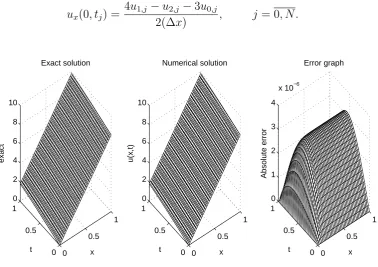
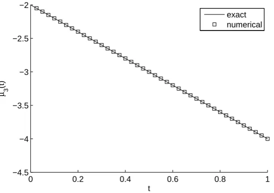
The numerical and exact solutions for the temperatureu(x, t) at interior points are shown in Figure 1 and one can observe that an excellent agreement is obtained. Figure 2 shows the numerical solution in comparison with the exact one for µ3(t) and the curves look indistinguishable. The x-partial derivative of u(x, t) at x = 0 has been evaluated using the followingO(h2_{) finite-difference approximation formula:}

ux(0, tj) =

4u1,j−u2,j−3u0,j

2(∆x) , j = 0, N . (47)

0 0.5

1

0 0.5 1 0 2 4 6 8 10

x Exact solution

t

exact

0 0.5

1

0 0.5 1

0 2 4 6 8 10

x Numerical solution

t

u(x,t)

0 0.5

1

0 0.5 1 0 1 2 3 4

x 10−6

x Error graph

t

Absolute error

0 0.2 0.4 0.6 0.8 1 −4.5

−4 −3.5 −3 −2.5 −2

µ 3

(t)

t

exact numerical

Figure 2: Exact and numerical solutions for the heat flux µ3(t) of the Dirichlet direct problem obtained withM =N = 40.

3.2

The Neumann direct problem

The FDM analysis for the direct (the inverse of the Inverse Problem II) initial Neumann boundary value problem given by equations (2), (6) and (24) is similar to that of direct Dirichlet problem of previous subsection. In this case, we discretise equations (38), (2) and (24) as:

ui,j+1−ui,j

∆t =

1

2(Gi,j +Gi,j+1), i= 0, M , j = 0,(N −1), (48)

ui,0 =ϕ(xi), i= 0, M , (49)

u−1,j−u1,j =−2(∆x)ν1(tj), uM+1,j−uM−1,j = 2(∆x)ν2(tj), j = 1, N , (50)

where Gi,j is given by (40), and u−1,j and uM+1,j for j = 1, N are fictitious values at

points located outside the computational domain. Equations (48) can be rewritten in the form of the system (43) for i = 0, M, j = 0,(N −1). At each time step tj+1 for j = 0,(N −1), using the Neumann boundary conditions (50), we obtain aM×M system of linear equations of the form,

˜

D˜uj+1 = ˜Eu˜j+ ˜b, (51)

where

˜

uj+1 = (u0,j+1, u1,j+1, ..., uM,j+1)tr,

˜

D=



     

1 +B0,j+1 −2C0,j+1 0 · · · 0

−C1,j+1 0

0

D

... −CM−1,j+1

0 · · · 0 −2CM,j+1 1 +BM,j+1



     

˜ E =       

1−B0,j 2C0,j 0 · · · 0

C1,j 0

0

E

... CM−1,j

0 · · · 0 2CM,j 1−BM,j

       , and ˜ b=        ∆t

2 (f0,j+f0,j+1)−2(∆x)(C0,jν1(tj) +C0,j+1ν1(tj+1)) ∆t

2 (f1,j+f1,j+1) ...

∆t

2 (fM−1,j+fM−1,j+1)

∆t

2 (fM,j +fM,j+1) + 2(∆x)(CM,jν2(tj) +CM,j+1ν2(tj+1))

       .

In the above expressions the matrices ˜D and ˜E contain the matrices D and E of the Dirichlet direct problem defined in subsection 3.1.

3.2.1 Example

As an example, consider the direct problem (2), (6) and (24) with T =L= 1 and

a(t) = 1 +t, b(x) = 2−x2, ϕ(x) = u(x,0) =x+ sin(x), ν1(t) =−ux(0, t) =−2, ν2(t) = ux(1, t) = 1 + cos(1),

f(x, t) = 8 + (1 +t)(2−x2) sin(x).

The exact solution is given by (45) and the desired boundary temperature output (25) is

µ1(t) =u(0, t) = 8t. (52)

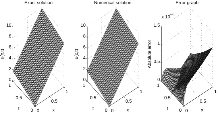
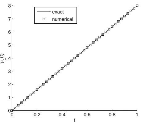
The numerical and exact solutions for the temperatureu(x, t) at interior points are shown in Figure 3 and one can observe that an excellent agreement is obtained. Figure 4 shows excellent agreement between the numerical solution and the exact one for µ1(t).

0 0.5 1 0 0.5 1 0 2 4 6 8 10 x Exact solution t u(x,t) 0 0.5 1 0 0.5 1 0 2 4 6 8 10 x Numerical solution t u(x,t) 0 0.5 1 0 0.5 1 0 0.5 1 1.5

x 10−4

x Error graph

t

Absolute error

0 0.2 0.4 0.6 0.8 1 0

1 2 3 4 5 6 7 8

µ 1

(t)

t exact numerical

Figure 4: Exact and numerical solutions for µ1(t) of the direct Neumann problem obtained withM =N = 40.

4

Solution of Inverse Problems

We wish to obtain stable and accurate reconstructions of the time-dependent thermal conductivitya(t) and the temperatureu(x, t) satisfying the equations (2)–(4) and (6) for Inverse Problem I, and equations (2), (6), (24) and (25) for Inverse Problem II.

The most common approach based on imposing the measurement (4) or (25) in a least-squares sense, is minimizing

FI(a) :=

a(t)ux(0, t) +µ3(t)

2

+βa(t)

2

, (53)

for Inverse Problem I, and

FII(a) :=

u(0, t)−µ₁(t)

2 +β

a(t)

2

, (54)

for Inverse Problem II, where β ≥ 0 is a regularization parameter to be prescribed and the norm is usually the L2_{[0, T]-norm. The discretization of (53) and (54) yields}

FI(a) = N

∑

j=0

[

ajux(0, tj) +µ3(tj)

]2

+β

N

∑

j=0

a2j, (55)

FII(a) = N

∑

j=1

[

u(0, tj)−µ1(tj)

]2

+β

N

∑

j=0

a2_j, (56)

wherea= (aj)j=0,N. It is worth mentioning that in (55) at the first time step, i.e. j = 0,

the derivativeux(0,0) is obtained from the initial condition (2), via (47), as

ux(0,0) =

4ϕ1−ϕ2−3ϕ0

where ϕi = ϕ(xi) for i = 0, M. Also, in (56), the value of a(0) can be obtained by

differentiating condition (25) with respect tot and using equation (1) atx= 0, namely,

a(0) = µ

′

1(0)−f(0,0)

b(0)ϕ′′₍₀₎ . (58)

The minimization of the objective function (55), or (56), subjected to the physical simple lower bound constraintsa >0 is accomplished using the MATLAB toolbox routine lsqnonlin, which does not require supplying (by the user) the gradient of the objective function, [16].

This iterative routine attempts to solve a nonlinear least-squares minimization prob-lem, starting from an initial guess, subject to constraints, and this generally is referred to as a constrained nonlinear optimization. We use the Trust-Region-Reflective (TRR) op-timization algorithm from lsqnonlin [16] and the positive components of the vector a are sought in the interval (10−10_,103_{). The algorithm is based on the interior-reflective} New-ton method, [4, 5], and some details about how this is implemented for the minimization of a least-squares functional like (55), or (56), has recently been given in [10].

In the numerical implementation, we take the parameters of the routine lsqnonlinas follows:

• Number of variables M =N = 40.

• Maximum number of iterations = 102_{×(number of variables).}

• Maximum number of objective function evaluations = 103_{×(number of variables).}

• Solution Tolerance (aTol) = 10−20_÷10−15_.

• Object function Tolerance (FunTol) = 10−20_÷10−15_.

• Nonlinear constraint tolerance = 10−6_.

The inverse problems under investigation are solved subjected to both exact and noisy heat flux measurement, (4) or (25) for Inverse Problems I and II, respectively. The noisy data is numerically simulated as

µϵk(tj) =µk(tj) +ϵ( k)

j , j = 0, N , k ∈ {1,3}, (59)

whereϵj are random variables generated from a Gaussian normal distribution with mean

zero and standard deviation σk given by

σk =p× max

t∈[0,T]|µk(t)|, k∈ {1,3}, (60)

where p represents the percentage of noise. We use the MATLAB function normrnd to generate the random variablesϵk =

(

ϵ(jk)

)

j=0,N as follows:

ϵk=normrnd(0, σk, N + 1). (61)

The total amount of noise ϵk is given by

ϵk =

ϵ_k

=

v u u t

N

∑

j=0 (µϵ

k(tj)−µk(tj))2, k ∈ {1,3}. (62)

In the case of noisy data (59), we replace µ3(tj) by µϵ3(tj) forj = 0, N in (55) and µ1(tj)

byµϵ

5

Numerical Results and Discussion

In this section, we present a few test examples to illustrate the accuracy and stability of the numerical scheme based on the FDM combined with the minimization of the least-squares functional (55), or (56), as described in Section 4. In order to explain the accuracy of the numerical results we introduce the root mean square error (rmse), defined as

rmse(a) =

v u u t

1 N + 1

N

∑

j=0

(anumerical(tj)−aexact(tj))2. (63)

We takeL=T = 1 and present the numerical results obtained with M =N = 40. Unless otherwise specified, we take the initial guess as a(0) _{= 1.}

5.1

Numerical Results for Inverse Problem I

We consider a couple of examples for the Inverse Problem I. Before we present the numer-ical results, we mention that regularization has not been found necessary and hence we considerβ = 0 in the functional (55). Thus was to expected since, according to Theorem 3, the Inverse Problem I is stable in the C[0, T] maximum norm with respect to small errors in the input dataµϵ

3.

5.1.1 Example 1

In this example, we consider the inverse problem (2)-(4) and (6) with the input data

ϕ(x) =u(x,0) =x+ sin(x), b(x) = 2−x2_,

µ1(t) =u(0, t) = 8t, µ2(t) =u(1, t) = 1 + sin(1) + 8t,

f(x, t) = 8 + (1 +t)(2−x2) sin(x), µ3(t) =−a(t)ux(0, t) = −2−2t.

One can observe that the conditions of Theorems 1 and 2 are satisfied hence the problem is uniquely solvable. The analytical solution is given by

a(t) = 1 +t, u(x, t) = x+ sin(x) + 8t. (64)

0 2 4 6 8 10 10−25

10−20 10−15 10−10 10−5 100 105

Number of Iterations

Objective function

Figure 5: The objective function (55), for Example 1 with no noise.

0 0.2 0.4 0.6 0.8 1

0.8 1 1.2 1.4 1.6 1.8 2

t

a(t)

iter 0 iter 1 iter 2,3, ... , 10 exact

Figure 6: The thermal conductivitya(t), for Example 1 with no noise.

0 2 4 6 8 10

10−4 10−3 10−2 10−1 100

Number of iterations

rmse(a)

0.5809

0.0062

0.0002

0.0002

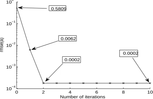
Figure 7: The rmse values of a(t), versus the number of iterations, for Example 1 with no noise.

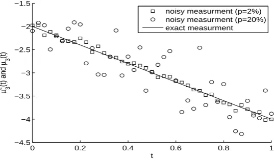
total amount of noise that is applied is ϵ3 ∈ {0.3540,3.5392}, respectively, as defined by equation (62). Figure 8 represents the exactµ3(t) and a typical noisy measurement input data µϵ

3(t).

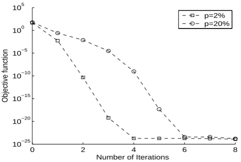
Figure 9 represents the objective functional (55), as a function of number of iterations,

when p∈ {2%,20%}. From this figure it can be seen that a very fast decreasing

conver-gence is achieved for p ∈ {2%,20%} in 8 iterations each, to reach a stationary value of O(10−24_).

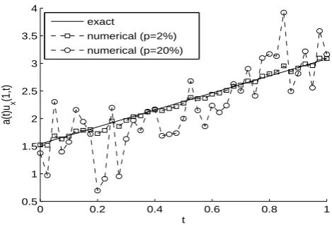
Figures 10–12 show the numerical solutions for the thermal conductivitya(t), the heat fluxa(t)ux(1, t) at x= 1, and the rmse(a) values, respectively, for p∈ {2%,20%} noise.

From these figures, as well as Figure 6, it can be seen that the numerical solution for the thermal conductivitya(t) converges to the exact solution a(t) = 1 +t, as the percentage of noise p decreases from 20% to 2% and then to 0. The nonlinear least-squares mini-mization produces good and consistent retrievals of the solution even for a large amount of noise such as 20%. In Figure 12, forp= 20% a slight ’semi-convergence’ phenomenon seems to appear after a couple of iterations, but this is more likely to be attributed to a non-monotonic decreasing convergence rather than to the former phenomenon which is commonly encountered when solving ill-posed problems iteratively, [8]. That is to say, our inverse problem is rather stable and in fact, as mentioned before at the beginning of Section 5.1, no regularization was needed to be included in the least-squares functional (55).

Finally, Figure 13 shows the exact solution, the numerical solution for the temperature u(x, t) and the relative error between them. From this figure it can be seen that the numerical solution is stable and furthermore, its accuracy is consistent with the amount of noise shown in Figure 8, which was included into the input data (4).

0 0.2 0.4 0.6 0.8 1

−4.5 −4 −3.5 −3 −2.5 −2 −1.5

µ 3

ε (t) and

µ 3

(t)

t

noisy measurment (p=2%) noisy measurment (p=20%) exact measurment

0 2 4 6 8 10−25

10−20 10−15 10−10 10−5 100 105

Number of Iterations

Objective function

p=2% p=20%

Figure 9: The objective function (55), for Example 1 with p∈ {2%,20%} noise.

0 0.2 0.4 0.6 0.8 1

0.8 1 1.2 1.4 1.6 1.8 2 2.2

t

a(t)

iter 0 iter 1 iter 2, 3,... exact

(a)

0 0.2 0.4 0.6 0.8 1

0 0.5 1 1.5 2 2.5

t

a(t)

iter 0 iter 1 iter 2, 3 ... exact

(b)

0 0.2 0.4 0.6 0.8 1 0.5

1 1.5 2 2.5 3 3.5 4

a(t)u

x

(1,t)

t exact

numerical (p=2%) numerical (p=20%)

Figure 11: The exact and numerical heat flux a(t)ux(1, t), for Example 1 with p∈ {2%,20%}

noise.

0 2 4 6 8

0 0.1 0.2 0.3 0.4 0.5 0.6 0.7

Number of iterations

rmse(a)

p=2% p=20%

Figure 12: The rmse values of a(t), versus the number of iterations, for Example 1 with

0 0.5 1 0 0.5 1 0 2 4 6 8 10 x Exact solution t exact 0 0.5 1 0 0.5 1 0 2 4 6 8 10 x Numerical solution t u(x,t) 0 0.5 1 0 0.5 1 0 0.02 0.04 0.06 x t

Relative error (%)

(a) 0 0.5 1 0 0.5 1 0 2 4 6 8 10 x Exact solution t u(x,t) 0 0.5 1 0 0.5 1 0 2 4 6 8 10 x Numerical solution t u(x,t) 0 0.5 1 0 0.5 1 0 0.2 0.4 0.6 x t

Relative error (%)

(b)

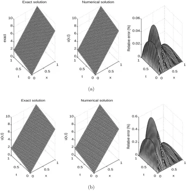
Figure 13: The exact and numerical temperature u(x, t), for Example 1 with (a) p = 2% and (b)p= 20% noise. The relative error between them is also included.

5.1.2 Example 2

In the previous example we have inverted the unknown thermal conductivitya(t) = 1 +t which is a smooth function. In this example, we consider a non-smooth test function, see equation (65). We consider the inverse problem (2)–(4) and (6) with the following input data

ϕ(x) =u(x,0) =xex, b(x) = 2−x2, µ1(t) =u(0, t) =t2, µ2(t) =u(1, t) =e+t2, µ3(t) =−a(t)ux(0, t) = −1−

t− 1 2 ,

f(x, t) = 2t−

( 1 + t− 1 2 )

(2−x2)(xex_{+ 2e}x_).

One can notice that the conditions of Theorem 2 are satisfied hence the uniqueness of the solution holds. With this data, the analytical solution of the Inverse Problem I is given by

a(t) = 1 + t−

1 2

, u(x, t) =xe

We study the case of exact and noisy input data (4). The objective function (55), as a function of the number of iterations, is presented in Figure 14. Form this figure it can be seen that the same fast decreasing convergence is achieved as in Example 1.

The numerical results for the corresponding time-dependent thermal conductivitya(t), the heat flux a(t)ux(1, t), the rmse(a) values and the interior temperature u(x, t) are

presented in Figures 15–18, respectively. The same conclusions as those obtained for Example 1 can be drawn by observing these figures.

0 2 4 6 8 10

10−30 10−20 10−10 100 1010

Number of Iterations

Objective function

p=0 p=2% p=20%

0 0.2 0.4 0.6 0.8 1 0.9

1 1.1 1.2 1.3 1.4 1.5 1.6

t

a(t)

iter 0 iter 1 iter 2, 3, ..., 9 exact

(a)

0 0.1 0.2 0.3 0.4 0.5 0.6 0.7 0.8 0.9 1 0.9

1 1.1 1.2 1.3 1.4 1.5 1.6

t

a(t)

iter 0 iter 1 iter 2, 3, ..., 8 exact

(b)

0 0.2 0.4 0.6 0.8 1

0.5 1 1.5 2 2.5

t

a(t)

iter 0 iter 1 iter 2, 3, ..., 6 exact

(c)

Figure 15: The thermal conductivity a(t), for Example 2 with (a) p = 0, (b) p= 2% and (c)

0 0.2 0.4 0.6 0.8 1 4

5 6 7 8 9 10

a(t)u

x

(1,t)

t exact (p=0) (p=2%) (p=20%)

Figure 16: The exact and numerical heat fluxa(t)ux(1, t), for Example 2 withp∈ {0,2%,20%}

noise.

0 2 4 6 8 10

−0.05 0 0.05 0.1 0.15 0.2 0.25 0.3 0.35

Number of iterations

rmse(a)

p=0 p=2% p=20%

Figure 17: The rmse values of a(t), versus the number of iterations, for Example 2 with

0 0.5 1 0 0.5 1 0 1 2 3 4 x Exact solution t exact 0 0.5 1 0 0.5 1 0 1 2 3 4 x Numerical solution t u(x,t) 0 0.5 1 0 0.5 1 0 0.2 0.4 0.6 0.8 1 x t

Relative error (%)

(a) 0 0.5 1 0 0.5 1 0 1 2 3 4 x Exact solution t exact 0 0.5 1 0 0.5 1 0 1 2 3 4 x Numerical solution t u(x,t) 0 0.5 1 0 0.5 1 0 5 10 15 x t

Relative error (%)

(b)

Figure 18: The exact and numerical temperature u(x, t), for Example 2 with (a) p = 2% and (b)p= 20% noise. The relative error between them is also included.

Numerical outputs such as the number of iterations and function evaluations, as well as the final value of the convergent objective function are provided in Table 1 for both Examples 1 and 2.

Table 1: Number of iterations, number of function evaluations, value of objective function (55) at final iteration, for Examples 1 and 2 withp∈ {0,2%,20%}noise.

Example Numerical outputs p= 0 p= 2% p= 20%

1

No. of iterations 10 8 8

No. of function evaluations 451 328 328

Function value 1.7E−24 1.1E−24 1.6E −24

rmse(a) 1.7E−4 0.0282 0.2809

2

No. of iterations 9 7 6

No. of function evaluations 369 287 246

Function value 5.8E−27 7.4E−27 2.8E −26

5.2

Numerical Results for Inverse Problem II

We now consider a couple of examples for the Inverse Problem II. Unlike for the Inverse Problem I which has been found stable with respect to noise in the input data (4), for the Inverse Problem II regularization was found necessary to be included in the functional (56) in order to obtain stable numerical solutions. This is to be expected since in the stability estimate (26) of Theorem 6, the right-hand side term contains the noisy data (µϵ

1−µ1) in theC1[0, T]-norm which where differentiated produce an unstable numerical solution.

5.2.1 Example 3

In this example, we consider the inverse problem (2), (6), (24) and (25) with the input data

ϕ(x) =u(x,0) = 1 +xex_{, b(x) = 2−x}2_, ν1(t) =−ux(0, t) = −1, ν2(t) =ux(1, t) =−2e,

f(x, t) =et−(1 +t)(2−x2)(xex+ 2ex), µ1(t) =u(0, t) = et.

One can observe that the conditions of Theorem 5 are satisfied hence, a solution is unique. The analytical solution is given by

a(t) = 1 +t, u(x, t) =xex_+et_{. (66)}

We start the investigation with exact input data (25), i.e. there is no noise included. Figure 19 represents the evolution of objective functional (56), as a function of the num-ber of iterations, with no regularization, i.e. β = 0. From this figure it can be seen that a fast decreasing convergence is achieved in 7 iterations to reach a very low value of order O(10−26_{). The corresponding numerical results of the time-dependent thermal} conductivity a(t) are displayed in Figure 20. From this figure it can be seen that there is an excellent agreement between the exact and numerical solutions with an rmse(a)= 0.0086.

0 2 4 6 8

10−30

10−20

10−10

100

1010

Number of Iterations

Objective function

0 0.2 0.4 0.6 0.8 1 0.8

1 1.2 1.4 1.6 1.8 2 2.2

t

a(t)

exact numerical

Figure 20: The thermal conductivity a(t), for Example 3 with no noise and no regularization.

In order to test the stability of the problem, we addp= 2% random Gaussian additive noise as in (59) which, according to (62), yields the total amount of noise ϵ1 = 0.2314. Let us denote by

RII(a) = N

∑

j=1

[u(0, tj)−µϵ1(tj)]2, (67)

the least-squares residual associated to the regularized Tikhonov functional (56).

Figure 21 shows the residual functional (67), as a function of the number of iterations, for various regularization parameters β ∈ {0,10−3_,10−2_,10−1_{}. From this figure one can} observe that convergence is rapidly achieved for each value of β. The resulting thermal conductivity is plotted in Figure 22 for various regularization parameters. As expected, when no regularization is employed, i.e. β = 0, the estimated a(t) is highly unstable and inaccurate. This shows that the Inverse Problem II is ill-posed. Consequently, a small perturbation in input data (25) causes a drastic error in the output solutiona(t). In order to overcome this instability, we employ the Tikhonov regularization method with β >0. From Figure 22 and Table 2, it can be observed that the stability is indeed restored and the value ofβ =O(10−2_{) produces the most accurate numerical results.}

100 101 102

10−2

10−1

100

101

102

103

Number of Iterations

Residual functional

β=0

β=10−3

β=10−2

β=10−1

0 0.1 0.2 0.3 0.4 0.5 0.6 0.7 0.8 0.9 1 0

1 2 3 4 5 6

t

a(t)

exact

β=0

β=10−3

β=10−2

β=10−1

Figure 22: The thermal conductivity a(t), for Example 3 with p = 2% noise and various regularization parameters.

0 0.5 1 0 0.5 1 0 2 4 6 x Exact solution t u(x,t) 0 0.5 1 0 0.5 1 0 2 4 6 x Numerical solution t u(x,t) 0 0.5 1 0 0.5 1 0 0.05 0.1 0.15 x Error graph t Relative error(%) (a) 0 0.5 1 0 0.5 1 0 2 4 6 x Exact solution t u(x,t) 0 0.5 1 0 0.5 1 0 2 4 6 x Numerical solution t u(x,t) 0 0.5 1 0 0.5 1 0 0.02 0.04 0.06 0.08 0.1 x Error graph t Relative error(%) (b) 0 0.5 1 0 0.5 1 0 2 4 6 x Exact solution t u(x,t) 0 0.5 1 0 0.5 1 0 2 4 6 x Numerical solution t u(x,t) 0 0.5 1 0 0.5 1 0 0.02 0.04 0.06 0.08 0.1 x Error graph t Relative error(%) (c) 0 0.5 1 0 0.5 1 0 2 4 6 x Exact solution t u(x,t) 0 0.5 1 0 0.5 1 0 2 4 6 x Numerical solution t u(x,t) 0 0.5 1 0 0.5 1 0 0.1 0.2 0.3 x Error graph t Relative error(%) (d)

5.2.2 Example 4

Consider the inverse problem (2), (6), (24) and (25) with the input data

ϕ(x) = u(x,0) = ex_{, b(x) = 2−x}2_,

ν1(t) = −ux(0, t) = −et, ν2(t) =ux(1, t) =e1+t,

f(x, t) = ex+t−(1 + 2πcos(2πt)2)(2−x2)ex+t, µ1(t) =u(0, t) =et. The analytical solution is given by

a(t) = 1 + 2πcos2(2πt), u(x, t) =ex+t_{. (68)}

For this thermal conductivity the initial guess was a0 = 1 + 2π. The objective function (56), as a function of the number of iterations, is depicted in Figure 24 for no noise and no regularization. From this figure it can be seen that the objective function (56) with β = 0, i.e the residual functional (67), is decreasing over several orders of magnitude, as the number of iterations increases, reaching a very low value of O(10−15_{) after 400} iterations. The computational time taken by the lsqnonlin to produce this convergence was about 10.6 minutes. The resulting thermal conductivity is shown in Figure 25 and very good agreement between the exact and numerical solutions can be observed.

100 101 102 103

10−20

10−15

10−10

10−5

100

105

Number of Iterations

Objective function

Figure 24: The objective function (56), for Example 4 with no noise and no regularization.

0 0.1 0.2 0.3 0.4 0.5 0.6 0.7 0.8 0.9 1

1 2 3 4 5 6 7 8

t

a(t)

exact numerical

Next, the input data (25) was perturbed by p = 2% noise. The residual function (67), as a function of the number of iterations, and the numerical results for a(t) are plotted in Figures 26 and 27, respectively, for various regularization parameters β ∈

{0,10−3_,10−2_,10−1_{}. As in Example 3, one can see that the numerically obtained results}

forβ= 0 in Figure 27 are unstable being highly oscillatory and unbounded. However, the inclusion of some regularization with β > 0 in the objective functional (56) restores the stability of the numerical solution, as shown further in Figure 27. One can observe that the choice β = 10−1 _{is too large and it oversmooths the solution, whilst the choice β = 10}−3

is too small and it undersmooths the solution. It seems that a regularization parameter β of O(10−2_{) realizes the desired compromise of balancing the under- and over-smooth} regions. Finally, Figure 27, as well as Figure 22 for Example 3, give some insight about how one may choose the regularization parametersβ >0. Based on practical experience, on can start with a rather large values forβ, and then decrease it until oscillations in the numerical solution start to appear [7].

100 101 102 103

10−2

10−1

100

101

102

103

Number of Iterations

Residual functional

β=0

β=10−3

β=10−2

β=10−1

Figure 26: The residual function (67), for Example 4 with p = 2% noise and various regular-ization parameters.

0 0.1 0.2 0.3 0.4 0.5 0.6 0.7 0.8 0.9 1

0 2 4 6 8 10 12

t

a(t)

exact

β=0

β=10−3

β=10−2

β=10−1

Figure 27: The thermal conductivity a(t), for Example 4, with p = 2% noise and various regularization parameters.

evaluations, the final value of the convergent objective function, as well as the rmse(a) are provided in Table 2 for Examples 3 and 4.

The numerical results for the temperature u(x, t) were found, as in Figure 23 for Example 3, accurate and stable and therefore they are not presented. Finally, although not illustrated, it is reported that an accurate and stable retrieval also was obtained for a non-smooth thermal conductivity.

Table 2: Number of iterations, number of function evaluations, value of regularized ob-jective function (56) at final iteration, and the rmse(a) for Examples 3 and 4 with β ∈ {0,10−3_,10−2_,10−1_{}and p= 2% noise.}

Example Numerical outputs β = 0 β = 10−3 _{β = 10}−2 _{β = 10}−1

3

No. of iterations 97 63 51 70

No. of function evaluations 4116 2688 2184 2982

Function value 0.0455 0.1818 1.0574 8.7697

rmse(a) 1.2697 0.6829 0.3158 0.4836

4

No. of iterations 976 49 41 42

No. of function evaluations 40016 2016 1764 1806

Function value 0.0286 1.029 8.917 73.817

rmse(a) 2.4973 0.7479 0.7135 1.7179

6

Conclusions

A couple of inverse problems which require determining a time-dependent thermal con-ductivity when the spacewise dependent heat capacity is given for the heat parabolic equation under overspecified conditions have been investigated. The Inverse Problem I given by equations (2)–(4) and (6) was found to be well-posed, whilst the Inverse Problem II given by equations (2), (6), (24) and (25) was found to be ill-posed and needed regu-larization in order to obtain a stable solution. A direct solver based on a Crank-Nicolson finite difference scheme has been developed. The inverse solver is based on a nonlinear least-squares minimization which has been solved numerically using the MATLAB tool-box routinelsqnonlin. Numerical results illustrated for several benchmarks test examples show that an accurate and stable solution has been obtained.

Future work will consider extending the present study to the simultaneous identifica-tion of several time-dependent parameters in the reacidentifica-tion-diffusion-convecidentifica-tion equaidentifica-tion, [12].

Acknowledgments. M.S. Hussein would like to thank the Higher Committee of Edu-cation Development in Iraq (HCEDiraq) for their financial support in this research. The authors would like to thank Professor M. Ivanchov for discussions on the topic of this work.

References

Park, California.

[2] Cannon, J.R. and DuChateau, P. (1973) Determining unknown coefficients in a non-linear heat conduction problem,SIAM Journal on Applied Mathematics,24, 298–314.

[3] Cannon, J.R. and Rundell, W. (1991) Recovering a time-dependent coefficient in a parabolic differential equation, Journal of Mathematical Anaysis and Applications,

160, 572–582.

[4] Coleman, T.F. and Li, Y. (1994) On the convergence of interior-reflective Newton methods for nonlinear minimization subject to bounds,Mathematical Programming,

67, 189–224.

[5] Coleman, T.F. and Li, Y. (1996) An interior trust, region approach for nonlinear minimization subject to bounds,SIAM Journal on Optimization, 6, 418–445.

[6] Doris, H.G., Peralta, J. and Luis, E.O. (2013) Regularization algorithm within two parameters for the identification of the heat conduction coefficient in the parabolic equation,Mathematical and Computer Modelling, 57, 1990–1998.

[7] Dennis, B.H., Dulikravich, G.S. and Yoshimura, S. (2004) A finite element formu-lation for the determination of unknown boundary conditions for three-dimensional steady thermoelastic problems, Journal of Heat Transfer, 126, 110–118.

[8] Elfving, T., Nikazad, T. and Hansen, P.C. (2010) Semi-convergence and relaxation parameters for a class of SIRT algorithms, Electronic Transactions on Numerical Analysis, 37, 321–336.

[9] Ismailov, M.I. and Kanca, F. (2012) The inverse problem of finding the time-dependent diffusion coefficient of the heat equation from integral overdetermination data, Inverse Problems in Science and Engineering, 20, 463-476.

[10] Ito, K. and Liu, J.-C. (2013) Recovery of inclusions in 2D and 3D domains for Poisson’s equation,Inverse Problems,29, 075005 (20 pages).

[11] Ivanchov, M.I. (1997) Inverse problem of finding a major coefficients in a parabolic equation,Matematychni Studii, 8, 212–220.

[12] Ivanchov, M.I. (2000) Inverse problem of simultaneous determination of two coeffi-cients in a parabolic equation,Ukrainian Mathematical Journal, 52, 379–387.

[13] Ivanchov, M.I. (2003)Inverse Problems for Equations of Parabolic Type, VNTL Pub-lications, Lviv, Ukraine.

[14] Lesnic, D., Yousefi, S.A. and Ivanchov, M. (2013) Determination of a time-dependent diffusivity from nonlocal conditions,Journal of Applied Mathematics and Computing,

41, 301–320.

[16] Mathworks R2012 Documentation Optimization Toolbox-Least Squares (Model Fit-ting) Algorithms, available from www.mathworks.com/help/toolbox/optim/ug /brnoybu.html.

[17] Wang, Y., Yang, C. and Yagola, A. (2011)Optimization and Regularization for Com-putational Inverse Problems and Applications, Springer-Verlag, Berlin.

[18] Wang, P. and Zheng, K. (2002) Determination of an unknown coefficient in a nonlin-ear heat equation,Journal of Mathematical Analysis and Applications,271, 525–533.