An active contour algorithm for spectrogram track detection

This is a repository copy of

An active contour algorithm for spectrogram track detection

.

White Rose Research Online URL for this paper:

http://eprints.whiterose.ac.uk/46266/

Version: Accepted Version

Article:

Lampert, Thomas and O'Keefe, Simon orcid.org/0000-0001-5957-2474 (2010) An active

contour algorithm for spectrogram track detection. Pattern Recognition Letters. pp.

1201-1206.

https://doi.org/10.1016/j.patrec.2009.09.021

[email protected]

Reuse

Items deposited in White Rose Research Online are protected by copyright, with all rights reserved unless indicated otherwise. They may be downloaded and/or printed for private study, or other acts as permitted by national copyright laws. The publisher or other rights holders may allow further reproduction and re-use of the full text version. This is indicated by the licence information on the White Rose Research Online record for the item.

Takedown

If you consider content in White Rose Research Online to be in breach of UK law, please notify us by

An Active Contour Algorithm for Spectrogram Track

Detection

Thomas A. Lampert∗

, Simon E. M. O’Keefe

Department of Computer Science, University of York, Heslington, York, United Kingdom, YO10 5DD

Abstract

This paper proposes an active contour framework for spectrogram track detec-tion. A potential energy is proposed which results in feature extraction at a signal-to-noise ratio (SNR) of 0.5 dB. We show, through complexity analysis, that this is achievable in real-time.

Key words: Active contour, Periodic time series, Remote sensing, Low signal-to-noise ratio, Spectrogram, Statistical pattern recognition

1. Introduction

Remotely sensed time series data is conventionally transformed into the fre-quency domain using the Fast Fourier Transform. This allows for the con-struction of a spectrogram image in which time and frequency are the axes and intensity is representative of the series’ power at a particular time and frequency. It follows from this that, if a stationary or non-stationary periodic component is present during some consecutive time frames a track, or line, will be present within the spectrogram.

The problem of automatic detection of these tracks drew increasing atten-tion in the literature during the mid 1980s and research expanded during the 1990s and early 21st _{century. Existing applications cover a wide range and}

include meteor detection, identifying and tracking marine mammals via their calls (Urazghildiiev and Clark, 2007), identifying noise radiated by mechanical devices (Yang et al., 2002; Chen et al., 2000) and distinguishing events such as ice cracking (Ghosh et al., 1996) and earth quakes (Howell et al., 2003). In the broad sense this “problem arises in any area of science where periodic phenom-ena are evident and in particular signal processing” (Quinn, 1994). In practical terms the problem can form a critical stage in the analysis of any noisy time series data, for example identifying trends in temperature variation and sea

∗_{Corresponding author. Tel.: +44 (0)1904 432794; fax: +44 (0)1904 432767.}

level rise and fall in altimeter data. Possible future applications include light frequency analysis through spectroradiometry and chemical detection through spectroscopy.

The active contour model (also known as a snake) proposed by Kass et al. (1988) allows for non-parametric feature detection within an image – ideal in remote sensing environments where generallya priori shape information is not strictly defined. The active contour is constrained by internal energy forces, which ensure that its shape follows certain criteria; these are typically defined as curvature and connectivity. It is guided by potential energy which attracts it towards features by following local changes in energy gradient. As these gra-dients are calculated on a local basis the active contour needs to be initialised close to the desired feature to ensure correct convergence. The active contour converges on a minimum of the weighted combination of its internal and po-tential energies. The popo-tential energy constraints translate this convergence to be a local gradient maxima in the image. However, the dependence on defining image features by gradient inhibits its applicability in low signal-to-noise ratio (SNR) conditions (Lampert et al., 2009).

The following extends previously published work (Lampert and O’Keefe, 2008) by including a detailed algorithm description, an analysis of complexity, a thorough evaluation using a greater number of test cases, an investigation into parameter value sensitivity, application to tracks with temporal instability and an evaluation upon real data. Unfortunately, it is not possible to present an algorithm comparison as there is no publicly available benchmark dataset for the application. To aid future comparisons, the data used for testing the proposed method is thoroughly described.

This paper is laid out as follows: in Section 2 the active contour model is outlined for single and multiple track detection and a complexity analysis is presented. In Section 3 experimental results are presented which demonstrate the success and limitations of these implementations, and in Section 4 our con-clusions are drawn.

2. Method

This section presents the active contour model applied to single and multiple feature detection and an analysis of the algorithm’s complexity.

2.1. The Active Contour Model

The original active contour model, as proposed by Kass et al. (1988), is as follows. A collection ofkcontour points,v(t) = [x(t), y(t)],t∈ {0,1, . . . , k−1}, forms a deformable contour wherex(t) andy(t) are the contour point’s position in the spectrogramS= [sij]M×N such thatx(t)∈ {0,1, . . . , N−1} andy(t)∈

{0,1, . . . , M−1}. The contour has the energy

E(v) =

k−2

X

t=1

α|v′

(t)|2+β|v′′

wherev′

(t)≈v(t)−v(t+1) andv′′

(t)≈v(t−1)−2v(t)+v(t+1) denote the dis-crete approximation of the contour’s first and second derivatives (respectively) with respect to t, the terms α and β control the continuity and curvature of the contour (respectively) and the termP is the potential induced by the image (otherwise known as the external energy).

The potential is defined to attract the contour to lines or edges in the image. The simplest features for this are the image intensity,P(v(t)) =−γsx(t),y(t), or

gradient,P(v(t)) =−γ

∇sx(t),y(t)

2

, where∇is the gradient operator andγis the potential’s weight.

2.2. Active Contour Model for Spectrogram Track Detection

The active contour model described here is an open ended contour where the first and last points are fixed to the top and bottom of the spectrogram such that v(0) = [x(0), ρ] and v(k−1) = [x(k−1), M−ρ], where ρis the height dimension of the potential energy defined below. Movement is restricted in the y-axis to ensure an even search along this axis.

2.2.1. Walk Force

To overcome the first limitation of the original active contour model, its sensitivity to the initialisation location, a walk force W can be implemented (Lampert and O’Keefe, 2008), such that

W(v(t)) =

−c

0

v(t). (2)

This forces the contour, with forcec, to perform an even search throughout the spectrogram after being initialised at a low frequency.

2.2.2. Potential Energy

The very low SNR exhibited in spectrograms highlights the algorithm’s sec-ond limitation, the use of image features which are unreliable at such SNRs. We propose forming an energy term which combines intensity information with spatial information to allow for detection along broken (weak) tracks. To accom-plish this, an energy term derived from intensity values taken within aξ×ρpixel window Wij_{, centred on pointv(t) = [x(t), y(t)] where i=x(t) andj =y(t),}

is proposed. The intensity values are arranged column wise into a vectorVij and PCA is utilised to derive a compact feature vector which represents the window. Its similarity to noise can be measured by testing its membership of a noise model. To allow its use as a potential energy, the measure has to be formulated to take a maximum value when the window contains a signal track and minimum value when the window contains noise.

We define a noise model as a multivariate Gaussian distribution fitted to noise windows projected ontodprincipal componentsU, such that

G(v(t)) = 1 (2π)d2|Σ|12

e−1

2Q

T

−0.6 −0.4 −0.2 0 0.2 0.4 0.6 0.1

0.2 0.3 0.4 0.5 0.6 0.7 0.8 0.9 1

1.1 Noise

3 dB SNR 6 dB SNR

Gaussian Response Contours

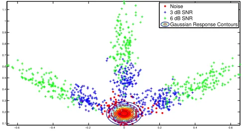
Figure 1: Windowed spectrogram feature vectors projected onto the first 2 principal compo-nents (window size 21×_{3 pixels). The noise class is represented by red circular points, the}

two signal classes, having a SNR of 3 and 6 dB, by blue and green crosses respectively and the contours represent the Gaussian distribution. Increasing the tracks SNR increases its distance from the noise class. The three pronged fan structure results from the track being present in the left, middle or right of the window.

forQ=UT_Vx(t)y(t)_{−µ whereµand Σ the mean and standard deviation of}

the noise cluster.

This results in a distribution similar to that presented in Fig. 1, in which there is a clear separation of the classes and in which the noise can be easily modelled using a Gaussian distribution.

Single Track Detection. The noise model’s response can be used as a potential energy in the active contour’s definition. First a threshold ǫ is defined which represents the confidence that a point within this range is a member of the noise class – simplifying the active contour’s feature space, such as

E(v(t)) =

1, ifG(v(t))≥ǫ

G(v(t)), otherwise. (3)

This is combined with the walkforce defined earlier to replaceP in Eq. (1), such that

P(v(t)) =W(v(t)) +γE(v(t)). (4)

130 260 20 40 60 80 100 120 140 Frequency (Hz) Time (s) 0 0.1 0.2 0.3 0.4 0.5 0.6 0.7 0.8 0.9 1

(a) Single track, as defined in Eq. (4). 130 260 20 40 60 80 100 120 140 Frequency (Hz) Time (s) 0 0.1 0.2 0.3 0.4 0.5 0.6 0.7 0.8 0.9 1

(b) Multiple tracks, as defined in Eq. (5) (h= 5 andc= 0).

Figure 2: Potential energy topologies for a 150×150 pixel section of a spectrogram (excluding

the walkforce). The x-axis represents frequency, the y-axis time and intensity energy. For easier interpretation the values here are 1−_P(v(t)), making the valleys peaks and vice-versa.

The parameters used to generate this data areǫ= 0.00008 and a window size of 3×21 pixels.

Frequency (Hz)

T

ime (s)

1 2 3 4 5 6 7 8

5 10 15 20 25 30 35 40

Figure 3: Contour mesh configuration, the contour ‘body’ in circles, its harmonic set locations defined byPsin squares and lines depicting the connection of potential energy.

Multiple Track Detection. Simultaneous tracks originating from a common so-urce can have some underlying linear relationship, for example, periodic signals are made up of harmonic frequencies and produce tracks in a spectrogram at harmonic locations (non-linear harmonics can also be present but these are not dealt with here). A priori knowledge regarding harmonic relationships can be exploited to improve detection reliability, especially at low SNRs. This knowl-edge can take the form of a pattern set Ps = [f q1, . . . , f qh], where f qi is a

multiple of the fundamental frequency, and can be integrated into the potential energy function, Eq. (4), such that

P(v(t)) =W(v(t)) + γ

h+ 1 "

E(v(t)) +

h

X

i=1

E

f qi 0

0 1

v(t) #

(5)

wherehis the number of relative frequencies inPs. Window samples in Eq. (5)

are taken from relative locations as defined inPsand the potential energy forms

a pattern-based active contour search – an active ‘mesh’ (Fig. 3).

Frequency (Hz)

Time (s)

0 1 2 3 4 5 6 7 8 0

10 20 30 40

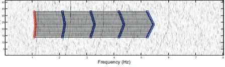
Figure 4: An example of a 2 dB SNR spectrogram image representing 39.5 seconds of data. Tracks are located at 1.2 Hz, 2.4 Hz, 3.6 Hz, 4.8 Hz and 6.0 Hz.

corresponding to the fundamental frequency of the signature pattern and this is easily distinguished from the weaker harmonic response. Gaps in the track have been interpolated with information from higher harmonics and false positive detections are weaker due to the random nature of noise.

2.3. Algorithm Complexity

The complexity of the presented algorithm is linear in all parameters except the PCA space dimension.This non-linearity is a result of computing the inverted matrixΣ−1 _{in Eq. (3) which has a time complexity of}

O(n3) using Gaussian elimination and can be reduced to O(n2.376_{) using more complex algorithms}

(Duda et al., 2000). However, asΣ−1 _{does not vary during run-time its value}

can be calculated and stored prior to execution, reducing this complexity to

O(n2). Additionally, the matrix multiplication QTΣ−1 _{in Eq. (3) is processed}

inO(n2) asQTis a 1×dmatrix andΣ−1_{is and×dmatrix (matrix multiplication}

between ann×mmatrix and anm×dmatrix isO(nmd) – in this casem=d

and n = 1 so the order is O(n2)). We have found that 2 or 3 PCA vectors capture sufficient information, therefore this non-linearity is acceptable.

3. Experimental Results

The proposed method has been tested using 340 spectrograms generated from synthetic time-domain signals, described by the pattern setPs= [2,3,4,5],

10 20 30 40 50 60 0

1 2 3 4 5 6 7x 10

23

Principal Component

−0.5 dB SNR 1.5 dB SNR 2.5 dB SNR

Figure 5: Eigenvalues associated with the principal components derived by averaging over 10 random training sets, each containing 1000 examples of each class. The red line represents the eigenvalues for 2.5 dB SNR examples, the green 1.5 dB SNR and the blue -0.5 dB SNR and error bars of 2 standard deviations (SNRs are rounded to the nearest 0.5 dB).

1 2

3 5

10 15 20 −0.2 −0.1 0 0.1 0.2

1st Principal Component

1 2

3 5

10 15 20 −0.2 −0.1 0 0.1 0.2

2nd Principal Component

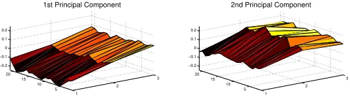
Figure 6: The first two principal component vectors viewed as 21×3 point surface plots.

3.1. Algorithm Parameters

The PCA vectors were derived from a training set containing 1000 noise and 1000 signal and noise feature vectors from a 0 dB SNR spectrogram with a window size of 21×3 pixels. Consequently, SNRs greater than 0 dB will be better separated from the noise class than when deriving principal components from higher SNR vectors. Plotting the PCA eigenvalues of data sets having SNRs of−0.5, 1.5 and 2.5 dB shows that a large amount of the data’s variance is captured within the first two principal components, Fig. 5. For the ‘straight track’ case, two dimensions sufficiently represent the data. The distribution is shown in Fig. 1. Surface views of the principal component vectors confirms PCA’s ability to capture salient information from this data, Fig. 6. The first is similar to the Prewitt, first derivative, edge detector (Prewitt, 1970) and the second, a second partial derivative edge detector,s′′

ij=si−1,j−2sij+si+1,j.

The algorithm’s sensitivity to different parameter values was investigated experimentally. The mean detection rate of the algorithm over a training set containing 34 spectrograms with straight tracks and SNRs of -0.8 to 7.6 dB was calculated with different parameter values. The results are presented in Fig. 7. The potential energy provides the information to locate features in an image. Its weight is controlled by the parameterγand as this increases the active contour gains more information from the image. This is reflected in the detection rates, asγincreases the detection rate also increases. The internal energy parameters

0 0.1 0.2 0.3 0.4 0.5 0.6 0.7 0.8 0.9 1 0

0.2 0.4 0.6 0.8 1

Parameter Value

Detection Rate

α β γ c

Figure 7: Algorithm sensitivity to parameter value variation (results obtained by averaging over 2 random training sets). Whilst each of the parameters was varied the remaining took the following values: α= 0.1,β= 0.2,γ= 1,k= 20,c= 0.41 andǫ= 0.00008.

0 1 2 3 4 5 6 7

0 0.2 0.4 0.6 0.8 1

SNR

Detection Rate

Straight Track Sloped Track Sinusoidal Track

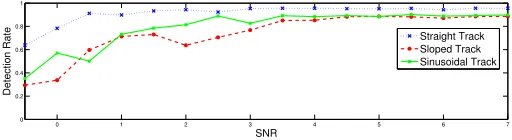
Figure 8: Proportion of patterns detected having less than 5 pixels difference with decreasing SNRs. Results are the average of 10 repetitions on different spectrograms with the same SNR (SNRs are rounded to the nearest 0.5 dB).

β has a far greater effect, at low values the contour has sufficient freedom to model track variations and evolve, however, when the influence is too great this is restricted and the contour is not able to evolve and model the tracks. The walk forcec enables the active contour to locate features which lie outside its local gradient topology and to pass over false positive detections which result from the potential energy. It is observed that asc increases, i.e. the contour moves over false positives with a greater force, detection rates also increase. However, if the value is too great the contour begins to move over true positives and the detection rates decrease. For the remainder of the experiments, unless otherwise stated, the following parameter values are used: the number of contour points is set tok= 20, taking the average position of these when a detection is made, the internal energy parameters are set toα= 0.1 andβ= 0.2, the potential energy parameter toγ = 1, the walk force to c= 0.41 and the Gaussian threshold to

ǫ= 0.00008.

3.2. Results

Frequency

Time

1.3 2.6 3.9 5.2 6.5 7.8 9.1 10.4 50

100 150 200 250

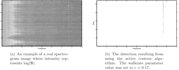
(a) An example of a real spectro-gram image where intensity rep-resents log(S).

Frequency

Time

1.3 2.6 3.9 5.2 6.5 7.8 9.1 10.4 50

100 150 200 250

(b) The detection resulting from using the active contour algo-rithm. The walkrate parameter value was set toc= 0.17.

Figure 9: An example of real spectrogram track detection.

were obtained; at all SNRs, on average, a pattern is detected within 1 pixel of its true location.

The algorithm was applied to the example of real data presented in Fig. 9(a), an underwater recording of a fishing vessel,1 and the result is presented in Fig. 9(b). The method successfully detects the single track present in the spec-trogram. The detection contains gaps where the track fades as there are no harmonics present to augment the missing information (which would be the case in multiple track detection). It also demonstrates the method’s ability to model small fluctuations in the frequency position of the track.

4. Conclusions

In this paper we have presented an active contour framework with applica-tion to the detecapplica-tion of single and multiple tracks in spectrograms – a critical step in the remote detection of a wide variety of periodic phenomena. The ben-efits of this model are; its use of past data anda priori structure information to enhance the detection process and its computational simplicity. Includinga priori knowledge of a pattern structure allows the detection of tracks at very low SNRs, typically less than 1 dB in short time frames. The model also com-bines the tracking (in short time frames) and detection process into one stage, simplifying the problem. If detection is performed at each time step, and thus the algorithm is used solely as a detection mechanism, this allows for a greater amount of information to be passed to a tracking stage.

The presented method uses a Gaussian noise model, classifying anything at the extreme as signal. This is useful as the characteristics of the signal can vary greatly. However, this means that any unknown clutter in the image, not

1_{This spectrogram is available as part of our spectrogram analysis data set, which is}

conforming to the noise distribution, is classified as signal. This can be overcome by fitting a distribution to the signal class, if it is well defined, and using its output as an additional negative energy component.

The following limitations of the proposed method have been identified; the need to identify the relationship between simultaneous tracks originating from a common source, the simplicity of the noise model and the separation of crossing tracks. The first of these issues only occurs when the relationship is not defined by integer harmonics, in that casea priori knowledge of the system may reveal the relationships or methods from the machine learning domain could be applied to identify them. The second, regarding the simplicity of the noise model, limits the algorithm’s application in real spectrograms as background noise which is time variant is not currently accounted for. Clutter can also confuse the algo-rithm, which is true for all state of the art systems, however, we have proposed possible solutions to this. The last point that is raised concerns crossing tracks, it can be the case that two sources exist and the track of one crosses the track of the other. This poses the problem of correctly associating the detected points to each track. These issues are currently being investigated and will be addressed in future research.

Although the presented quantitative results are derived using synthetic data, experiments upon real data have been performed under similar SNRs producing similar positive results (due to the nature of these data the results can not be presented). An example of the algorithm working in real conditions has been presented to illustrate this.

Acknowledgements

This research has been supported by the Defence Science and Technol-ogy Laboratory (DSTL)1 _{and QinetiQ Ltd.}2_{, with special thanks to Duncan}

Williams1 _{for guiding the objectives and Jim Nicholson}2 _{for guiding the}

objec-tives and providing the synthetic data.

References

Chen, C.-H., Lee, J.-D., Lin, M.-C., 2000. Classification of underwater signals using neural networks. Tamkang J. of Science and Engineering 3 (1), 31–48.

Duda, R. O., Hart, P. E., Stork, D. G., 2000. Pattern Classification. Wiley-Interscience Publication.

Ghosh, J., Turner, K., Beck, S., Deuser, L., 1996. Integration of neural classifiers for passive sonar signals. Control and Dynamic Systems - Advances in Theory and Applications 77, 301–338.

Kass, M., Witkin, A., Terzopoulos, D., 1988. Snakes: Active contour models. Int. J. of Computer Vision 1 (4), 321–331.

Lampert, T. A., O’Keefe, S. E. M., December 2008. Active contour detection of linear patterns in spectrogram images. In: Proc. of ICPR’08. pp. 1–4.

Lampert, T. A., O’Keefe, S. E. M., Pears, N. E., May 2009. Line detection methods for spectrogram images. In: Computer Recognition Systems 3: Proc. of 6th Int. Conf. on Computer Recognition Systems CORES’09. Vol. 57 of Advances in Intelligent and Soft Computing. Springer-Verlag, pp. 137–145.

Prewitt, J. M. S., 1970. Picture Processing and Psychopictorics. Academic Press Inc., New York, NY, USA, Ch. Object Enhancement and Extraction, pp. 75– 149.

Quinn, B. G., May 1994. Estimating frequency by interpolation using Fourier coefficients. IEEE Trans. Signal Process. 42 (5), 1264–1268.

Urazghildiiev, I. R., Clark, C. W., August 2007. Acoustic detection of north at-lantic right whale contact calls using spectrogram-based statistics. The Jour-nal of the Acoustical Society of America 122, 769–776.