Three dimensional adaptive method for compressible multi-fluids flows

Three Dimensional Adaptive Method for Compressible

Multi-Fluids Flows

H. W. Zheng

and N. Qin

Department of Mechanical Engineering, University of Sheffield, Mappin Street, Sheffield S1 3JD, U.K

C. Shu

National University of Singapore, 10 Kent Ridge Crescent, Singapore 119260

In this paper, a hexahedral-mesh based solution adaptive algorithm for the simulation of compressible multi-fluid flows is proposed. The data structure, the refinement and coarsening process, and the solution adaptive method are described. The cells with different levels are stored in different lists. This avoids the recursive calculation of solution of mother (non-leaf ) cells. Besides, the faces are separated stored into two lists: one for leaf faces and another for non-leaf faces. Thus, high efficiency is obtained due to these features. Numerical results show that there is no oscillation of pressure and velocity across the interface and it is feasible to apply it to solve compressible multi-fluid flows with large density ratio (1000) and strong shock wave interaction with the interface.

Nomenclature

Af area of the facef E total energy

γ property of the material nf normal direction of the facef

U conservative variable vector p pressure

Φf numerical flux at the facef π property of the material

p∗j _{intermediate pressures}

r location of the initial interface r0 initial radius

ρ density

R residual vector

qf HLLC intermediate normal velocity sj intermediate signal speeds

S source vector t physical time u velocity vector ujn normal velocity Vc volume of cell c

∗_{Research Associate, Email: H.Zheng@sheffield.ac.uk.} †_{Professor of aerodynamics, and AIAA Associate Fellow.} ‡_Professor

48th AIAA Aerospace Sciences Meeting Including the New Horizons Forum and Aerospace Exposition

I.

Introduction

The compressible multi-fluid flows have been intensively investigated by many researchers.1–16 _{In general,} most of them are three dimensional. Besides, due to complexity of these problems such as steep material interface, density and pressure gradients that occur in such flows, accurate predictions of flow structure of compressible multi-fluid flows pose a major challenge. Thus, it is necessary to develop the three dimensional (3D) adaptive mesh technique to study the problems.

However, most work on compressible multi-fluid flows employ 2D Cartesian based adaptive method.6–9 For example,6, 8_{presented the work by combining the level set method and the 2D Cartesian adaptive meshes.} For this method, a complex modified coarse-to-fine and fine-to-coarse inter-level transfer operators need to be employed to stabilize the computation. Apart from Cartesian adaptive meshes, there is another paper9 which employs the 2D moving mesh method and real ghost fluid method.17 Their extension and applications to 3D compressible multi-fluid flows are still rarely conducted. In this paper, we extend the 2D quadrilateral based adaptive technique13 to 3D hexahedral based adaptive method.

The rest of the paper is organized as follows. In the second section, the governing equations are described. In the third section, the data structure, the criterion for refinement and coarsening and the solution adaptive method for compressible multi-fluid flows are presented. The numerical results are given in the fourth section.

II.

Governing equations

The governing equations for the compressible multi-fluid flows with stiffened gas equation of state (EOS) are Euler equations

∂t ∫ Ω    ρ ρu E   dV +

∫ ∂Ω    ρu

ρu⊗u+P[I] (E+P)u

 

·ndS= 0, (1)

whereρis the density,uis the velocity, andEis the total energy.

To tackle the well-known difficulty11, 14_{of spurious pressure oscillations at material interfaces, it requires} to solve another two transport equations

∂Ξ

∂t +u· ∇Ξ = 0. (2)

with, Ξ = ( β θ )

, β= 1 γ−1, θ=

γπ

γ−1 (3)

Here, β andθis a function of are the property of the material (γand π). β is also used to indicate the position of the interface. These two variables are also used to calculate the pressurepaccording to stiffened gas EOS,

p=

(

E−1 2ρu

2_+θ )

/β (4)

III.

Adaptive method

The adaptive grid generator developed in this work belongs to the unstructured adaptive grid family. In the following, the data structure, local refinement, local coarsening and the solution adaptive procedure are described.

A. Data structure

child cells as they can be accessed by using the sub-faces of the six faces. What is more, the neighboring cells of a cell can be obtained by visiting the six faces.

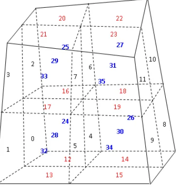
Figure 1. Data Structure

After each refinement of a cell, each cell is split into eight cells and each face of this cell is split into four sub-faces (Fig. 2). These cells are further organized into different lists according to their level and the faces are separated further stored into two lists: one for leaf faces and another for non-leaf faces. Specially care needs to be taken to reset the pointers to the new nodes of each face during the refinement (Fig. 3).

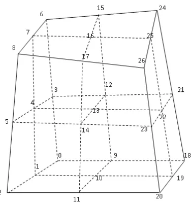
Figure 2. Faces created after refining a cell

B. Adaptive criterion for refinement and coarsening

Figure 3. Nodes created after refining a cell

error of density of each face,

εT = max f

(

|(∇lnρ)C−(∇lnρ)L| αfρC/dl+|(∇lnρ)L|

,|(∇lnρ)C−(∇lnρ)R| αfρC/dl+|(∇lnρ)R|

)

f

(5)

If the value of error detector of a target cell is greater than the pre-defined refining thresholdεR, then the cell needs to be refined; otherwise, if it is smaller thanεC, then the cell needs to be coarsened.

However, there are still two more constraints for the refinement process. One is that the cell has no children (sub-cells). The other one is that the maximum difference of the levels between the current cell and all the neighboring cells cannot be greater than one. Similarly, there are two more constraints for coarsening. The first one is that the cell must have children (sub-cells). The second one is that the maximum difference of the levels between the current cell and all the neighboring cells cannot be greater than one.

C. Solution adaptive method

In this method, in order to avoid the recursive calculation, the cells are separately stored in different lists according to their levels. Thus, the solution can be obtained in a level by level manner so that the cells of high level are calculated after the cells of low level.

1. Time evolution

The set of equation Eq. (1) can be easily discretized at each leaf cell by the two stage Runge-Kutta schemes,13

U(_c∗)=U_cn−αRes (U_cn) (6)

and

Un_c+1= 0.5

[

Un_c +U(_c∗)−αRc (

U(_c∗) )]

(7)

whereU is the state vector

(

ρ ρ⃗u E β θ

)T

, ∆tis the time step,Vc is the volume of cellc,Rc is the

residual, andαis the ratio between time step and the volume (α= ∆t/Vc).

2. Residual calculation

The face-based technique is employed to calculate the residual. That is, the residual (Rf1→L) at the left neighboring cell center (f1→L) of a leaf facef1 is updated in the following way,

Rf1→L= Rf1→L+ Φf1 (

U−,U+,nf1 )

and the residual (Rf1→R) at the right cell center (f1→R) of this leaf facef1 is updated by

Rf1→R=Rf1→R−Φf1 (

U−,U+,nf1 )

·Af1 (9)

In order to achieve the object of the spurious pressure oscillations-free material interfaces under complex geometry, the solving of the last two sub-equations in Eq. (1) are important. In this paper, we adopt a HLLC consistent way in paper,13 _{the HLLC scheme is embedded by updating the last two items of residue} as

RΞ,c=RΞ,c−Ξc

∑

f

qf·Af (10)

Here,qf is the HLLC intermediate normal velocity13 at the face.

3. Flux calculation

To discretize the convection term, the Harten, Lax and van Leer approximate Riemann solver with the Contact wave restored (HLLC) numerical flux for an facef is adopted for compressible multi-fluid flows,13

Φf

(

U−, U+,n)= 1 2

[

Φ−+ Φ+−sign(sm) (

U+−U−)] (11)

with

Φj =F(Uj)·n+s#_j (U∗j−Uj), j=−,+ (12)

where the intermediate states can be calculated by

U∗j= sj−u j n sj−sm

     ρj ρj[_uj₋(_uj

n−sm

) n] Ej Ξj     +      0 0 (

p∗j_sm−pj_uj n

)

/(sj−uj n ) 0    

, j=−,+ (13)

with

p∗j=ρj(uj_n−sj) (uj_n−sm)+pj, j=−,+ (14)

Here, sj andp∗j _{are the intermediate signal speeds and pressures of HLLC scheme.}13

IV.

Results and Discussion

In order to validate the performance of the present three-dimensional solution adaptive technique for compressible multi-fluid flows, test cases of material interface problem and bubble interaction with shock wave are considered herein.

4. Interface translation problem

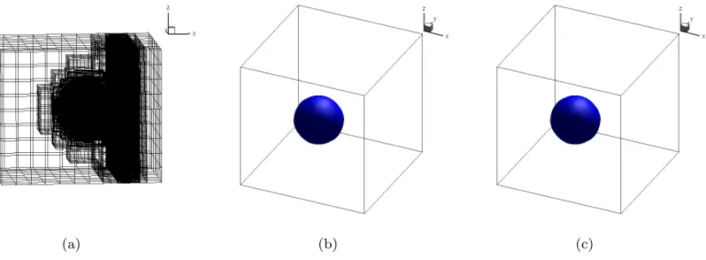
The interface translation problem is used to demonstrate the oscillation-free feature of current solver. Ini-tially, one fluid with a spherical shape surrounded by another fluid is put at the position (0.25m,0.25m,0.25m) of the domain. The radius of the spherical interface isr0= 0.16m. The periodic boundary condition is em-ployed at all boundaries. The initial mesh is adaptively generated by a 20×20×20 background mesh (level 0) with the finest resolution level as 4. The initial values of the primitive variables for the two fluids are given by,11

ρ1= 0.1kg/m3, u1= 1m/s, v1= 1m/s, w1= 1m/s, p1= 1P a, γ1= 1.4, π1= 0P a, f orr < r0 (15)

ρ2= 1kg/m3, u2= 1m/s, v2= 1m/s, w2= 1m/s, p2= 1P a, γ2= 1.6, π2= 0P a, f orr >=r0 (16)

It is used to verify the solver and see whether there is no oscillation of pressure and velocity across the interface.

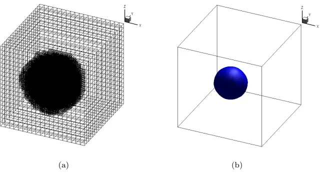
We plot the interface position at t=0 second and t=0.18 second as shown in Fig. 4 and Fig. 5. As stated above, the spherical interface moves with a constant velocity. Hence, there is an analytical solution for the interface position. From Fig. 4, it can be easily observed that the calculated position and shape of the interface at t=0.18 second agrees well with the predicted one.

(a) (b)

Figure 4. Mesh (a) and density iso-surface (b) at time t=0s

(a) (b)

Figure 5. Mesh (a) and density iso-surface (b) at time t=0.18s

Besides, the computed pressure and velocity are plotted in Fig. 6. It is clearly the pressure and velocity is uniform. These shows that they do not oscillate around the interface which confirms the claim of oscillation-free of our adaptive method.

5. Bubble-shock interaction

In this section, the bubble shock interaction with a large density ratio (1000) and pressure ratio between the water and gas bubble is investigated. Initially, a left going planar shock wave (Fig. 7) with Mach number of 1.422 traveling in the water and a circular bubble gas with radius of 0.2m are put at the left side (0.7m, 0.5m, 0.5m) of the shock wave. The domain is [0,1.2]×[0,1]×[0,1]m3 _{and the shock wave is located at} 0.95m.

The pre-shock and post-shock fluids are initially at rest and the parameters such as density, velocity, pressure and the material parameters are listed as follows,15, 16

(a) (b)

Figure 6. Slice of velocity (u) contour (a) and pressure contour (b) at time t=0.18s

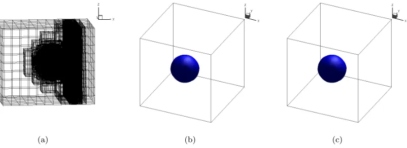
(a) (b) (c)

Figure 7. Mesh (a), density iso-surface (b) and interface iso-surface (c) at time t=0s

ρ3= 1230kg/m3, u3=−432.69m/s, v3= 0m/s, w3= 0m/s, p3= 109P a, γ3= 4.4, π3= 6·108P a (18)

The primitive variables for the bubble are set as,

ρ2= 1.2kg/m3, u2= 0m/s, v2= 0m/s, v2= 0m/s, p2= 105P a, γ2= 1.4, π2= 0.0P a (19)

The reflective boundary conditions are employed at the top and bottom boundary, while the extrapolation boundary conditions are imposed at the left and right boundary. This is a challenging problem due to the large pressure jump across the shock wave and the large ratio of the acoustic impedances of the liquid to gas.

The simulation is performed on the adaptive mesh generated by a uniform background mesh (level is 0) of 12×10×10 with the finest resolution level as 4. The mesh and the iso-surface of density andβ at different time from 0s to 0.0005s are plotted in Fig. 7 - 12.

(a) (b) (c)

Figure 8. Mesh (a), density iso-surface (b) and interface iso-surface (c) at time t=1e-4s

(a) (b) (c)

Figure 9. Mesh (a), density iso-surface (b) and interface iso-surface (c) at time t=2e-4s

V.

Conclusion

In this paper, a hexahedral based solution adaptive method for 3D compressible multi-fluid flows devel-oped is proposed. The approach is able to automatically and efficiently adjust the local mesh density to reflect the transient behavior of the solution. Two examples have been carried out to examine the perfor-mance of the present solver for compressible multi-fluid flows. They show the oscillation-free of pressure and velocity across the interface and it is feasible in solving compressible multi-fluid flows with large density ratio (1000) and strong shock wave (the pressure ratio is 10000) interaction with the interface.

References

1_{Larouturou, B., How to preserve the mass fraction positive when computing compressible multi-component flows, J.}

Comput. Phys., 95, 59-84, 1991.

2_{Abgrall, R., and Karni, S.,Computations of Compressible Multifluids, J. Comput. Phys., 169, 594-623, 2001.}

3_{Shyue, K.M.,An efficient shock-capturing algorithm for compressible multi-component problems, J. Comput. Phys., 142,}

208-242, 1998.

4_{Shyue, K.M.,A fluid-mixture type algorithm for barotropic two-fluid flow problems, J. Comput. Phys. 200, 718-748, 2004.} 5_{Johnsen, E. and Colonius, T.,Implementation of WENO schemes for compressible multicomponent flow problems, J.}

Comput. Phys., 219, 715-732, 2006.

6_{Nourgaliev, R.R., Dinh, T.N., and Theofanous, T.G.,Adaptive Characteristics-Based Matching for Compressible}

Multi-fluid Dynamics, J. Comput. Phys., 213, 500-529, 2006.

7_{Banks, J.W., Schwendeman, D.W., Kapila, A.K., and Henshaw W.D.,A high-resolution Godunov method for compressible}

multi-material flow on overlapping grids, J. Comput. Phys., 223, 262-297, 2007.

8_{Kadioglu, S.Y. and Sussman, M.,Adaptive solution techniques for simulating underwater explosions and implosions, J.}

(a) (b) (c)

Figure 10. Mesh (a), density iso-surface (b) and interface iso-surface (c) at time t=3e-4s

(a) (b) (c)

Figure 11. Mesh (a), density iso-surface (b) and interface iso-surface (c) at time t=4e-4s

9_{Wang, C., Tang H., and Liu, T.G.,An adaptive ghost fluid finite volume method for compressible gas-water simulations,}

J. Comput. Phys., 227, 6385-6409, 2008.

10_{Saurel, R., Gavrilyuk, S., and Renaud F., A multiphase model with internal degrees of freedom: application to}

shock-bubble interaction, JFM, 495, 283-321, 2003.

11_{Shyue, K.M.,An efficient shock-capturing algorithm for compressible multi-component problems, J. Comput. Phys., 142,}

208-242, 1998.

12_{Zhang, Q, Graham, M.J.,A numerical study of Richtmyer-Meshkov instability driven by cylindrical shocks, Phys. Fluids,}

10, 974-92, 1998.

13_{Zheng, H. W., Shu, C. and Chew, Y.T.,An Object-Oriented and Quadrilateral-mesh based Solution Adaptive Algorithm}

for Compressible Multi-fluid Flows, J. Comput. Phys., 227, 6895-6921, 2008.

14_{Abgrall, R., and Karni, S.,Computations of Compressible Multifluids, J. Comput. Phys. 169, 594-623, 2001.}

15_{Allaire, G, Clerc, S, and Kokh, S.,A five-equation model for the simulation of interfaces between compressible fluids, J.}

Comput. Phys., 181, 577-616, 2002.

16_{Shyue, K.M., A fluid-mixture type algorithm for compressible multicomponent flow with van der Waals equation of state,}

J. Comput. Phys., 156, 43-88, 1999.

17_{Wang, C.W., T.G. Liu, B.C. Khoo, A real-ghost fluid method for the simulation of multi-medium compressible flow,}

(a) (b) (c)