DOI: 10.1534/genetics.106.064618
Maximum-Likelihood Estimation of Allelic Dropout and False Allele
Error Rates From Microsatellite Genotypes in the
Absence of Reference Data
Paul C. D. Johnson
1and Daniel T. Haydon
Division of Environmental and Evolutionary Biology, Institute of Biomedical and Life Sciences, University of Glasgow, Glasgow G12 8QQ , United Kingdom
Manuscript received August 11, 2006 Accepted for publication December 5, 2006
ABSTRACT
The importance of quantifying and accounting for stochastic genotyping errors when analyzing mi-crosatellite data is increasingly being recognized. This awareness is motivating the development of data analysis methods that not only take errors into consideration but also recognize the difference between two distinct classes of error, allelic dropout and false alleles. Currently methods to estimate rates of allelic dropout and false alleles depend upon the availability of error-free reference genotypes or reliable ped-igree data, which are often not available. We have developed a maximum-likelihood-based method for estimating these error rates from a single replication of a sample of genotypes. Simulations show it to be both accurate and robust to modest violations of its underlying assumptions. We have applied the method to estimating error rates in two microsatellite data sets. It is implemented in a computer program, Pedant, which estimates allelic dropout and false allele error rates with 95% confidence regions from micro-satellite genotype data and performs power analysis. Pedant is freely available at http://www.stats.gla.ac. uk/paulj/pedant.html.
T
HE importance of quantifying and accounting for stochastic genotyping errors in microsatellite-based studies is becoming ever more widely recognized. Un-detected errors can impair inference across a range of fields, including forensics, genetic epidemiology, kin-ship analysis, and population genetics (Pompanonet al. 2005). All studies that have looked for genotyping errors have found them at appreciable levels (0.2–15% per locus; Pompanon et al. 2005). Even at low error rates, the frequency of erroneous genotypes increases rapidly with the number of marker loci assayed: from 1% in one locus, to 10% in 10 loci, to a potentially destructive 63% in 100 loci. Error-free microsatellite data sets must therefore be rare and will become rarer as improving laboratory methods allow increasing numbers of sam-ples and markers to be assayed. Thus, although errors are most obviously harmful when genotyping highly error-prone noninvasive samples (Gagneuxet al.1997), they can frustrate analysis of the cleanest data, for ex-ample, in mapping genes that contribute to complex disease (Feakes et al. 1999; Walters 2005). The con-sequences of undetected genotyping errors can be particularly adverse for parentage analysis, especially when using exclusion, where incompatibilities between candidate parents and offspring are used to exclude allbut the true parent (Gagneuxet al. 1997; Jonesand Ardren2003). Even an error rate as low as 2% in a nine-locus data set can result in false exclusion of .20% of fathers (Hoffmanand Amos2005).
Given that genotyping errors cannot be eliminated with certainty, a more pragmatic approach is to mini-mize (Piggottet al.2004), quantify (Boninet al.2004; Broquetand Petit2004; Hoffmanand Amos2005), and integrate them in statistical analysis (Marshall
et al.1998; Sobelet al.2002; Wang2004). Most studies quantify error rate as a single quantity, such as error rate per allele or per single-locus genotype. However, sto-chastic errors (as opposed to systematic errors, for ex-ample, null alleles) can be divided into two distinct classes:allelic dropout, where one allele of a heterozygote randomly fails to PCR amplify, andfalse alleles, where the true allele is misgenotyped because of factors such as PCR or electrophoresis artifacts or human errors in reading and recording data (Broquetand Petit2004). These two classes of error can bias analyses in funda-mentally different ways. For example, a high level of undetected allelic dropout could be misinterpreted as evidence for inbreeding, while false alleles can lead to substantial overestimation of census size (Waits and Leberg2000; Creelet al.2003).
The essential difference between the effects of the two classes of error, as far as kinship inference is concerned, is that both homozygotes and heterozygotes potentially contain false alleles, but only homozygotes
1Corresponding author: Robertson Centre for Biostatistics, Boyd Orr Bldg., University Ave., University of Glasgow, Glasgow G12 8QQ , United Kingdom. E-mail: [email protected]
can be suspected of allelic dropout. Consider a data set with a low false allele rate but a high allelic dropout rate, a common scenario for genotypes from noninvasive samples such as feces or hair (Broquet and Petit 2004). A candidate father with genotypeAAcould not be excluded with high confidence from paternity of an offspring with genotypeCCbecause of the high prob-ability of allelic dropout, but if the observed genotypes were AB and CD, respectively, the candidate father could be excluded with greater certainty. Thus, knowl-edge of both error rates allows the likelihood of pa-ternity to be assessed more accurately than is possible when using a single composite error rate. By the same logic, any microsatellite analysis that incorporates er-ror probability would benefit from differentiating be-tween allelic dropout and false alleles.
This approach is being increasingly applied to anal-ysis methods such as sibship reconstruction (Sieberts
et al.2002; Wang2004), parentage assignment (Hadfield
et al. 2006), and establishment of genotypic identity between two DNA samples (Kalinowskiet al.2006). By analyzing simulated data from 100 individuals at eight microsatellite loci, Wang(2004, Figure 2 therein) showed that sibships can be reconstructed accurately when the probabilities of allelic dropout and false alleles are as high as 20% each per single-locus genotype and only 3% of multilocus genotypes are expected to be error free.
The utility of such methods depends on the ability to quantify the separate error rates. Errors can be quanti-fied separately either through Mendelian inconsisten-cies between parent–offspring pairs or by comparing error-prone genotypes with reference genotypes, which are assumed to be error free. Reference genotypes can be obtained either from high-quality template DNA (but see Jefferyet al.2001) or by repeated PCRs (Ewen
et al.2000; Broquetand Petit2004; Pompanonet al. 2005). However, in many studies neither pedigree data nor reference samples will be available, and the pro-duction of reference data by multiple genotyping can be time consuming and expensive (Navidiet al.1992; Taberletet al. 1996; Smith et al. 2000; Milleret al. 2002). There is therefore a need to develop a method for estimating allelic dropout and false allele error rates that does not depend on pedigree data, high-quality reference samples, or multiple genotyping.
We describe a method for estimating maximum-likelihood rates of allelic dropout and false allele error from microsatellite genotype data. The method com-pares duplicate genotypes and estimates error rates on the basis of the frequency and nature of mismatches. It is already considered good practice to duplicate 5–10% of genotypes to monitor overall genotyping error (Bonin
et al.2004; Hoffmanand Amos2005; Pompanonet al. 2005), but it has not been possible to use these data to assess both allelic dropout and false alleles separately. The method presented here therefore extracts valuable information from data that researchers will often have
already obtained. Both duplicate genotypes are assumed to be error prone, so reference data are not required. We demonstrate the effectiveness of the method using simulated and real data.
METHODS
Notation and terminology: Genotyping error rates
are conventionally expressed per genotype rather than per allele, reflecting the fact that they are usually calculated in terms of the observed number of errone-ous genotypes ( judged against reference genotypes) divided by the number of genotypes in which an error could have been observed (Broquetand Petit2004). The per-genotype allelic dropout rate (p) is calculated as a proportion of observed heterozygotes (because allelic dropout can be observed only in heterozygotes) whereas the false allele rate (f) is calculated as a proportion of all genotypes. Per-genotype error rates are convenient to use and simple to calculate when reference genotypes are available but in the method presented here, which involves modeling the processes through which errors affect individual alleles, per-allele rates are more useful. In practice, conversion between allele and per-genotype rates is straightforward (seeappendix).
Using Wang’s (2004) notation for per-allele error rates,e1is the population allelic dropout rate ande2is the population false allele rate (defined below). Addi-tionally, we define the sample error rates, e1 and e2, which are the error rates in a single sample of replicate genotypes. For example, a sample of 200 duplicate genotypes contains 800 scored alleles. If 4 of these have dropped out thene1¼0.005, regardless of whether the dropouts occurred visibly in heterozygotes or invisi-bly in homozygotes. Finally, the error rate estimates are
^
e1and^e2.
Where ambiguity between true and error-prone geno-types is possible, we refer to the recorded error-prone genotype as the ‘‘observed genotype’’ and the unknown true genotype (which would be observed in the absence of errors) as the ‘‘underlying genotype.’’ An underlying genotype that has been ascertained by a process that is assumed to be error free is referred to as a ‘‘reference genotype.’’ In reality even reference genotypes can con-tain errors. Finally, unless stated otherwise, the term ‘‘genotype’’ refers to a single-locus genotype.
General approach: When reference genotypes are
Although errors can also be counted from a single set of duplicate genotypes in the absence of reference data, classifying them is more problematic because both rep-licate genotypes are error prone and allelic dropout and false alleles can produce equivalent mismatches (e.g., the mismatchAA.ABcould have been produced by allelic dropout in AB or the occurrence of a false allele inAA). However, information about the magni-tudes ofe1ande2can be derived from the frequencies
of different categories of mismatch. When e1 is high, AA.ABmismatches will be common, while a high fre-quency ofAB.ACmismatches indicates highe2.
A simple way to circumvent the ambiguity ofAA.AB
mismatches is to estimatee2ande1consecutively.AB.AC
mismatches are unambiguously attributable to false allele errors in heterozygotes and can be used to esti-mate e2 across the entire sample. This estimate of e2
can in turn be used to estimate the proportion ofAA.AB
observations expected to result from a false allele in a homozygote. The remainder of AA.ABduplicates can then be attributed to allelic dropout and used to esti-matee1. However, because both replicate genotypes are
error prone, the probability of both replicates incurring errors (a double error) is not negligible. If the total probability of an error of either class occurring in a sin-gle genotype (p1f) is a realistically high 0.2 (Broquet and Petit2004), then 5.2% of replicates will be hit by at least two errors, and these will account for 27% of errors. Ignoring these classes will result in substantial under-estimates of high error rates (we verified this result us-ing simulations—data not shown), and includus-ing them in the simple sequential approach described above be-comes impossible because of ambiguity in the origins of some categories of replicate genotype. For example, if double errors are considered, the apparently error-free
AA.AA category could arise from an underlying geno-type ofABby two dropouts, andAA.BBcould originate either fromABby two dropouts or fromAAby acquisi-tion of a false allele (B) followed by a dropout. Given these complications, rather than calculatinge2ande1
sequentially, it is preferable to estimate them simulta-neously from all the available data using maximum likelihood (ML). This method has the added advantage of allowing simple calculation of confidence limits.
There are seven possible categories of duplicate genotype: (1)AA.AA, (2)AB.AB, (3)AA.AB, (4)AA.BB, (5)AB.AC, (6)AB.CC, and (7)AB.CD. Categories that include two allelic dropouts in a single genotype are not counted because double dropouts are indistinguish-able from other causes of PCR failure and are there-fore unreliable indicators ofe1.
Like the simple sequential method described above for estimatinge1ande2without reference data, the basis
of the ML method is the sensitivity of categories 1–7 toe1
and e2. Assuming that the underlying proportion of
heterozygotes is known, the expected frequencies of all categories and the likelihood of the observed
frequen-cies can be calculated for any e1and e2, allowing the ML estimates,^e1and^e2, to be obtained.
Assumptions and model: We base our assumptions
and error model on those proposed by Wang(2004), with minor modifications. We make the following assumptions:
1. The genotypes are diploid and codominant.
2. The sampled population is in Hardy–Weinberg equilibrium.
This assumption is usually desirable because it allows expected heterozygosity (He¼1Pn
i¼1x 2
i, wherexi
is the frequency of theith ofnalleles) to be used to gauge the probability that an underlying genotype is heterozygous. In an error-free data set this probabil-ity is the observed heterozygosprobabil-ity (Ho), but direct estimates of Ho will be biased downward by allelic dropout and upward by false alleles. Neither dropout nor false alleles should significantly bias estimation of He, assuming that all alleles are equally likely to drop out and that false alleles generally do not cre-ate new allelic stcre-ates. A known degree of nonrandom mating can be accounted for by estimatingHofrom
HeandFIS, the inbreeding coefficient, whereHo¼ He(1 FIS). In practice, unbiasedFISestimates are unlikely to be available when errors are frequent, but in cases where the sample contains more than one population, heterozygote deficiency due to spatial genetic structure could be quantified and corrected for by replacing FIS with FST, which is relatively in-sensitive to genotyping error (Taberletet al.1999). We investigate the effect of undetected deviation from random mating on error rate estimation using simulations.
3. Each sample is equally likely to incur an error.In reality errors will preferentially affect low-quality samples (Pompanonet al.2005). The effect of nonindepen-dence among errors on both simulated and real data is explored and discussed below. Moreover, false al-leles might not affect homozygotes and heterozygotes with equal probability. For example, allele-calling errors are probably more likely in heterozygotes, whereas PCR artifacts are more likely to be recorded in homozygous genotypes. The confounding effect of such opposing biases could be overcome by model-ing false alleles as a product of two or more processes. However, to do so would require the introduction of at least one additional parameter at the cost of re-duced statistical power, increased mathematical com-plexity, and longer computing time.
5. A false allele always takes an allelic state not already present in the duplicate genotype. For example, an underlying genotype ABcan be duplicate genotyped asAB.CC
only by the occurrence in the second genotype of a false allele (C) in one allele followed by a dropout of the other allele, not by the occurrence of two identical false alleles. Likewise,AB.ABcan arise only by an error-free read of an underlyingAB, not by the same false allele (B) occurring in both genotypes from an underlying AA. In real data, most false al-leles are recorded as existing true alal-leles (P. C. D. Johnson, personal observation), so that in practice two identical false alleles could occur in a duplicate genotype in either theAB.CCor theAB.ABcase. This could lead to underestimation of highe2at loci with few alleles. However, given the high number of alleles present at most microsatellite loci and the relative rarity of double occurrences of false alleles, this rule is unlikely to lead to significant underestimation of
e2. A consequence of this assumption is that we do not include the number of alleles in a data set as a parameter in our model, which greatly simplifies the calculation of the expected duplicate genotype frequencies.
Following Wang’s (2004) error model, we define two classes of error. Class 1 consists of allelic dropouts only: each allele drops out with probabilitye1. Class 2 includes all stochastic errors that lead to a false allele being recorded, such as those caused by PCR and electropho-resis artifacts, allele miscalling either by software or by human error, and data entry. This class comprises all stochastic errors outside class 1. A false allele is recorded with probabilitye2. Systematic errors, which might be caused by null alleles, contaminant DNA, or systematic miscalling of an allele, are excluded from both classes. Thus in the production of a single diploid genotype, the probabilities of an error of classioccurring in neither allele, one allele, and both alleles are (1ei)2, 2ei(1ei),
andei2, respectively.
Our error model differs from Wang’s (2004) with respect to his assumption that dropouts always precede false allele errors when they occur together in a single allele, resulting in a heterozygous observed genotype (e.g.,ABdrops out toAA, which acquires a false allele to become AC). We reverse the order, so that dropouts overrule false alleles, leading to a homozygous observed genotype. For example, a dropout and a false allele would coincide in the second allele of an underlying
AAas follows: first AA acquires a false allele to be re-corded asABand then the false allele drops out to give
AA. Neither model perfectly fits reality: Wang’s order correctly models PCR artifacts that are mistaken for alleles, whereas ours fits any false allele that is able to drop out (e.g., miscalling or data entry errors). We chose to make dropouts dominant, first, because miscalling and data entry errors appear to be more common than
PCR artifacts, at least in high-quality data (Paetkau 2003; Bonin et al. 2004; Hoffman and Amos 2005; Pompanon et al. 2005), and, second, because it sim-plifies the calculation of the expected frequencies of the seven categories. In practice, this difference between the two models is slight, as the probability of both er-rors coinciding in at least one allele in a duplicate ge-notype is small even at very high error rates (0.05 when
e1¼0.17 ande2¼0.08).
We make a further simplifying assumption that at all realistic values of e2 the frequency of replicate
geno-types affected by three or four false allele errors is neg-ligible. This frequency is 0.2% when the false allele error rate is as high as 0.16 per single-locus genotype (equivalent to e2¼ 0.083), the highest recorded in a literature review by Broquetand Petit(2004), so this assumption seems justified.
Under the assumptions above, the expected fre-quency of each of the seven replicate genotype catego-ries is a function of three parameters: the error rates to be estimated,e1ande2, and the known expected
het-erozygosity,He. The likelihood of any combination ofe1
ande2can then be calculated, givenHeand the counts
of the seven categories (seeappendixfor derivation of equations). Calculating log likelihood across a suffi-ciently large number of error rate combinations allows a log-likelihood surface to be constructed and the ML estimates^e1and^e2 to be located (Figure 1).
A computer program, Pedant, that implements the above method was written in the programming lan-guage Delphi version 7.0 (Borland Software). Pedant automates the categorization of the replicate genotypes and finds the ML error rates using a simulated anneal-ing algorithm (seeappendixfor details). The advantage of simulated annealing is that it reduces the danger of the search getting stuck on a local maximum when searching likelihood space with multiple maxima. In practice, most, if not all, real data sets will produce unimodal surfaces resembling Figure 1. However, it is possible to create artificial data sets that produce two peaks, so it seems prudent to allow for this possibility in the search algorithm, particularly considering that the cost in computation time is small (typically ,1 sec/locus using 20,000 search iterations on a 3-GHz Celeron PC).
Simulations: We tested the method by estimating
errors from data with known error rates simulated under the assumptions of the error model. We then repeated the simulation analysis using data that violated the stronger assumptions of the error model. For each data set we generated n underlying genotypes, which were heterozygous with probabilityHe, and then simu-lated two observed genotypes each with error probabil-ities e1 and e2. Error rates were estimated from data
simulated with low (e1¼0.01,e2¼0.0015),
values of e1 and e2 were chosen to reflect a realistic range of genotyping error rates, from levels typical of high-quality samples (Ewen et al. 2000) to rates rep-resenting data from low-quality noninvasive samples (Broquetand Petit 2004). Other parameters tested were low (He¼0.5) and high (He¼0.85) expected het-erozygosities and small (n¼50), intermediate (n¼100), and large (n ¼ 200) sample sizes. Sampling error in
Hewas simulated as a function of Heand n, assuming a broken-stick distribution of allele frequencies (see appendix). All 54 possible combinations ofe1, e2,He, and n were simulated. Because generally only a frac-tion (e.g., 10%) of genotypes are replicated to calculate error rates, sampling error inHewas calculated for 10n
samples.
The performance of the method in estimating the population error rates was assessed by analyzing error rate estimates from 5000 simulated data sets. Perfor-mance was gauged by the mean square error (MSE) between the estimated (^e1 or ^e2) and the population
error rate (e1 or e2). The MSE can be split into two
components, bias and standard error (SE), where MSE¼
bias2 1 SE2. We calculated bias, relative bias, and standard error for each^e1 and^e2. Bias was calculated
as the mean estimated error rate minus the population error rate, and relative bias as bias divided by population error rate.
MSE depends not only on sampling error ine1ande2, but also on the number of hidden and ambiguous errors in the sample. The sample will have incurred on average 4ne1dropouts and 4ne2false alleles, so for any e1and
e2, how well the sample represents the population is therefore a function of n and not useful in assessing the performance of the method. Of greater interest is how well the method recovers the sample error rates in spite of the hidden and ambiguous errors, that is, what proportion of the error in the ML estimates is intrinsic to the method (intrinsic error) and not due to sampling error. Intrinsic error was calculated as (mean square error between the estimate and the sample error rate) divided by MSE. The closer that bias, MSE and intrinsic error were to zero, the better the method was judged to be performing.
The robustness of the method was tested by rerun-ning the performance analysis on simulated data sets that deviated from some assumptions of the error model in the following ways.
Deviation from Hardy–Weinberg equilibrium: The effect of undetected nonrandom mating within the sampled population was tested by simulating data at two levels of heterozygote deficiency, defined byFIS-values of 0.0625 and 0.125. TheseFIS-values equate to inbreeding among first cousins and half-siblings, respectively, and were chosen to represent moderate and high levels of in-breeding within wild vertebrate populations (Slate
et al. 2004). Heterozygote deficiency might also result from cryptic genetic structure. We concentrated on in-vestigating heterozygote deficiency (FIS. 0), first, be-cause extreme heterozygote excess (FIS , 0.125) is likely to be rare in nature (Figure 2 of Chesser1991) and, second, because preliminary simulation analysis suggested that the most severe biases are typically about three times smaller when FISis negative than when it is positive.
Increased sampling error in He: The method does not
take into account sampling error in He. The effect of increasing sampling error inHeto its maximum (when no additional samples are available for estimatingHe) was tested by decreasing the number of samples from whichHewas estimated from 10nton.
Sample quality variation: We investigated the validity of the assumption that each sample is equally likely to incur an error. This assumption is unlikely to hold true for most data sets: when sample quality varies, errors preferentially occur in low-quality samples (Gagneux
et al. 1997; Wandeler et al. 2003; Bonin et al. 2004; Pompanon et al. 2005). To test the effect of variable sample quality on error estimates, we simulated data using a nonuniform distribution of error rates across samples (seeappendix).
Dominance of dropouts over false alleles:The effect of the assumption that dropouts always hide false alleles was assessed by reducing the probability of a dropout hiding a false allele from 1 to 0.5 in the simulated data.
Figure1.—Maximum-likelihood (ML) estimates (1) and confidence regions for the population allelic dropout and false allele rates,e1ande2()). ML error rates were estimated from 100 simulated duplicate genotypes whereHe¼0.85,e1
¼0.05, ande2¼0.01. The seven duplicate genotype category
counts were (10, 67, 17, 2, 2, 0, 0) with two double dropouts uncounted. The sample error rates,e1ande2, are also shown
(h). Confidence regions were calculated by descending
x2
ð2;aÞ=2 log-likelihood units from the ML estimate, where
Reference data (e.g., consensus genotypes or pedigree data) are generally required to estimate allelic dropout and false allele error rates. Therefore, we tested the ML method against a reference data-dependent method. We compared the ML estimates with estimates that could have been obtained conventionally had one of the two duplicate genotypes been a reference genotype rather than an error-prone genotype. Thus the refer-ence data method has the advantage that visible errors are unambiguous, but the disadvantage of increased sampling error. The MSEs of the ML and reference data (RD) methods (MSEMLand MSERD) were compared for
both error rates. To allow this comparison the ML es-timates were converted from per-allele to per-genotype rates (seeappendix).
Application to real microsatellite data: The method
was tested on microsatellite genotypes from two error-prone sources of DNA: red fox teeth that had been autoclaved to denature rabies virus and fecal samples from Ethiopian wolves. Individual and consensus geno-types were kindly provided by P. Wandeler (foxes) and D. A. Randall (wolves).
For the fox samples, 149–182 consensus genotypes were established from up to nine repeated PCRs at 16 loci: V142, V374, V402, V468, V502, V602, V622 (Wandelerand Funk2006), AHT-130 (Holmeset al.
1995), CXX-156, CXX-250, CXX-279 (Ostrander
et al. 1993), CXX-434, CXX-466, CXX-606, CXX-608 (Ostranderet al.1995), and c2088 (Holmeset al.1995; Wandeler2004). Prior information from genetic data regarding the validity of assuming Hardy–Weinberg equi-librium in fox populations was not available, although using these data Wandeler(2004) found modest het-erozygote deficits within populations (FIS¼0.01–0.02) as well as low levels of interpopulation structure (FST¼
0.035). The assumption of Hardy–Weinberg equilib-rium was therefore unjustified in this data set. We did not correct for either source of heterozygote deficit becauseFISwould not normally be accurately quantifi-able prior to error estimation, and the same may apply to low levels ofFST (Boninet al. 2004). Simulation of error estimation under this total level of heterozygote deficit (FIT ¼ 0.05) predicted small biases of 3% in
^e1and8% in^e2.
For the wolf data set, 72–121 consensus genotypes were based on up to 19 repeated genotypes from 17 loci:
c377 (Ostrander et al. 1993), FH2001, FH2054,
FH2119, FH2137, FH2138, FH2140, FH2159, FH2174, FH2226, FH2293, FH2320, FH2422, FH2472, FH2537 (Breenet al.2001), Pez17, and Pez19 (Neffet al.1999). Ethiopian wolf microsatellites would not be expected to show significant deviation from Hardy–Weinberg equi-librium on the basis of prior information from other markers (Gottelli et al. 1994), and this has been confirmed using the present data (Randall2006).
The first two sets of repeat genotypes were analyzed using the ML method to give^e1 and^e2 with their 95%
confidence limits, the first set of genotypes providing the estimate ofHe. Error rate estimates and confidence limits were converted to per-genotype error rates for comparison with the sample error rates. The ML estimates were judged by their proximity to the true error rates in the sample, which were counted with reference to the consensus genotypes (with the excep-tion of dropouts in homozygotes, which are invisible even when reference data are available). Because pop-ulation error rates were not known, relative bias was calculated as (ML estimate)/(sample error rate when greater than zero). These data sets provide a thorough challenge for the ML method because, in addition to covering a wide range of He-values from 0.30 to 0.90 (meanHe-values: 0.79 in the foxes, 0.63 in the wolves), they also violate one of the stronger assumptions of the method in having a nonuniform distribution of error rates among samples.
RESULTS
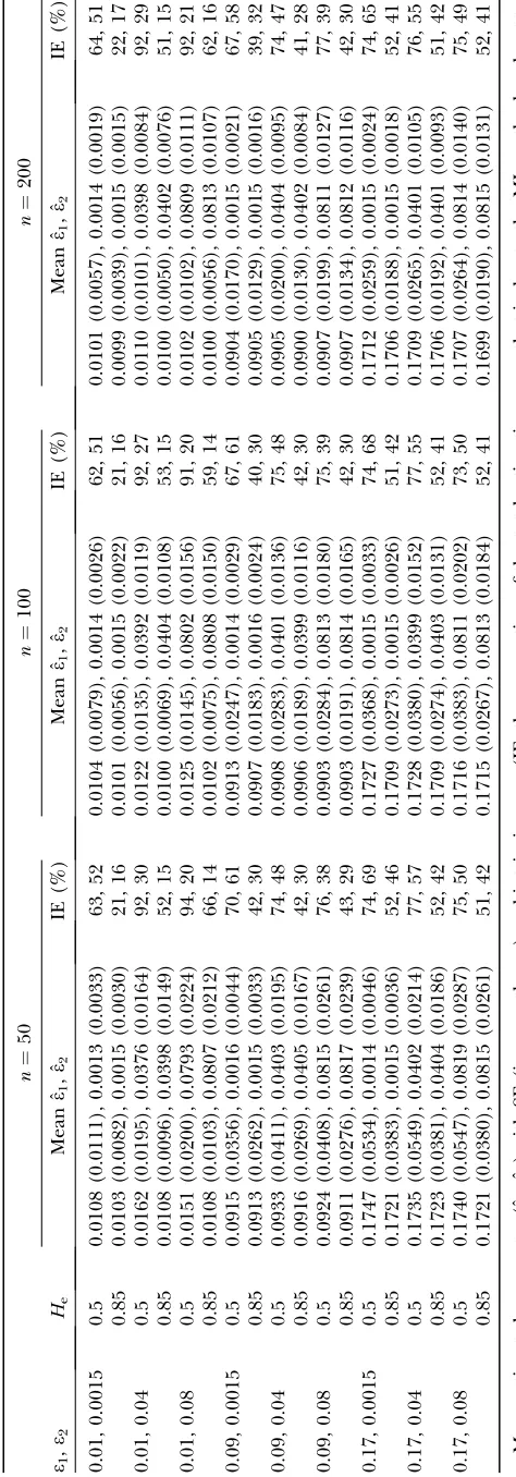
Simulations:The ML method performed well across
the full range of error rates, with rare exceptions, which are detailed below (Table 1). It performed best when Heand n were high and error rates were inter-mediate or high, that is, when the number of errors and the proportion of informative genotypes were high.
Bias: WhenHe¼0.85 andn¼200, relative bias was insignificant for both ^e1 and ^e2 across all error rate combinations (range 1.8–0.8%). However, relative bias increased with decreasing He and n (Figure 2) and was generally greater in^e1than in^e2. Although the magnitude of bias in^e1 was always low (range 0.0001– 0.0062), relative bias in^e1became high whenHe,n, and
e1were low (i.e., when the number of visible dropouts was low) ande2was high, reaching a maximum of 62% ate1¼0.01,e2¼0.04,He¼0.5, andn¼50 (Figure 2).
It appears that when the number of visible dropouts is low and the numbers of false alleles are high, some false alleles inAA.AB-type mismatches are ‘‘mistaken’’ for allelic dropouts. Although a bias of 62% in estimat-inge1of 0.01 may seem severe, high bias occurred only in circumstances where the data contained very few visible dropouts (e1¼0.01,He¼0.5,n¼50) and con-sequently was characterized by high sampling error, so that even the highest biases were overwhelmed by estimation error. The highest contribution of bias to MSE in^e1(bias2/MSE) was 9.1%, which occurred when bias was 62%. Bias in^e2 was always low, ranging from
15 to 2.6%. The largest bias, of 15%, was in es-timatinge2of 0.0015 atHe¼0.5 andn ¼50 and was responsible for only 0.4% of MSE.
T ABLE 1 Analysis of the perfor mance of the ML method in estimating allelic dropout and false allele er ro r rates fr om simulated data n ¼ 50 n ¼ 100 n ¼ 200 e1 , e2 He Mean ˆ e1 , ˆ e2 IE (%) Mean ˆ e1 , ˆ e2 IE (%) Mean ˆ e1 , ˆ e2 IE (%) 0.01, 0.0015 0.5 0.0108 (0.0111), 0.0013 (0.0033) 63, 52 0.0104 (0.0079), 0.0014 (0.0026) 62, 51 0.0101 (0.0057), 0.0014 (0.0019) 64, 51 0.85 0.0103 (0.0082), 0.0015 (0.0030) 21, 16 0.0101 (0.0056), 0.0015 (0.0022) 21, 16 0.0099 (0.0039), 0.0015 (0.0015) 22, 17 0.01, 0.04 0.5 0.0162 (0.0195), 0.0376 (0.0164) 92, 30 0.0122 (0.0135), 0.0392 (0.0119) 92, 27 0.0110 (0.0101), 0.0398 (0.0084) 92, 29 0.85 0.0108 (0.0096), 0.0398 (0.0149) 52, 15 0.0100 (0.0069), 0.0404 (0.0108) 53, 15 0.0100 (0.0050), 0.0402 (0.0076) 51, 15 0.01, 0.08 0.5 0.0151 (0.0200), 0.0793 (0.0224) 94, 20 0.0125 (0.0145), 0.0802 (0.0156) 91, 20 0.0102 (0.0102), 0.0809 (0.0111) 92, 21 0.85 0.0108 (0.0103), 0.0807 (0.0212) 66, 14 0.0102 (0.0075), 0.0808 (0.0150) 59, 14 0.0100 (0.0056), 0.0813 (0.0107) 62, 16 0.09, 0.0015 0.5 0.0915 (0.0356), 0.0016 (0.0044) 70, 61 0.0913 (0.0247), 0.0014 (0.0029) 67, 61 0.0904 (0.0170), 0.0015 (0.0021) 67, 58 0.85 0.0913 (0.0262), 0.0015 (0.0033) 42, 30 0.0907 (0.0183), 0.0016 (0.0024) 40, 30 0.0905 (0.0129), 0.0015 (0.0016) 39, 32 0.09, 0.04 0.5 0.0933 (0.0411), 0.0403 (0.0195) 74, 48 0.0908 (0.0283), 0.0401 (0.0136) 75, 48 0.0905 (0.0200), 0.0404 (0.0095) 74, 47 0.85 0.0916 (0.0269), 0.0405 (0.0167) 42, 30 0.0906 (0.0189), 0.0399 (0.0116) 42, 30 0.0900 (0.0130), 0.0402 (0.0084) 41, 28 0.09, 0.08 0.5 0.0924 (0.0408), 0.0815 (0.0261) 76, 38 0.0903 (0.0284), 0.0813 (0.0180) 75, 39 0.0907 (0.0199), 0.0811 (0.0127) 77, 39 0.85 0.0911 (0.0276), 0.0817 (0.0239) 43, 29 0.0903 (0.0191), 0.0814 (0.0165) 42, 30 0.0907 (0.0134), 0.0812 (0.0116) 42, 30 0.17, 0.0015 0.5 0.1747 (0.0534), 0.0014 (0.0046) 74, 69 0.1727 (0.0368), 0.0015 (0.0033) 74, 68 0.1712 (0.0259), 0.0015 (0.0024) 74, 65 0.85 0.1721 (0.0383), 0.0015 (0.0036) 52, 46 0.1709 (0.0273), 0.0015 (0.0026) 51, 42 0.1706 (0.0188), 0.0015 (0.0018) 52, 41 0.17, 0.04 0.5 0.1735 (0.0549), 0.0402 (0.0214) 77, 57 0.1728 (0.0380), 0.0399 (0.0152) 77, 55 0.1709 (0.0265), 0.0401 (0.0105) 76, 55 0.85 0.1723 (0.0381), 0.0404 (0.0186) 52, 42 0.1709 (0.0274), 0.0403 (0.0131) 52, 41 0.1706 (0.0192), 0.0401 (0.0093) 51, 42 0.17, 0.08 0.5 0.1740 (0.0547), 0.0819 (0.0287) 75, 50 0.1716 (0.0383), 0.0811 (0.0202) 73, 50 0.1707 (0.0264), 0.0814 (0.0140) 75, 49 0.85 0.1721 (0.0380), 0.0815 (0.0261) 51, 42 0.1715 (0.0267), 0.0813 (0.0184) 52, 41 0.1699 (0.0190), 0.0815 (0.0131) 52, 41 Mean estimated error rates (ˆ e1 ,
ˆe)2
Intrinsic error: Unsurprisingly, the standard error of the estimates was smallest at highn. More significantly, intrinsic error did not vary with n, but rather was sensitive to the two error rates andHe(Table 1, Figure 3). Like bias, intrinsic error was higher in^e1(21–94%)
than in^e2 (14–69%) and highest when estimating low e1at lowHeand highe2. AtHe¼0.85 intrinsic error in
^e1and^e2 averaged 46 and 29%, respectively, across the
range of simulated error rates and sample sizes, com-pared with 77 and 47% atHe¼0.5.
The simulation analysis above was carried out using data simulated under the assumptions of the error
model. We now show the effect of deviation from some of these assumptions.
Deviation from Hardy–Weinberg equilibrium: The only substantial effect of moderate (FIS¼0.0625) and high (FIS ¼ 0.125) heterozygote deficiency was to bias ^e1
and^e2. The relationship between FISand relative bias
was consistently linear across the range of parameter values tested. Relative bias in^e2was generally low, being FIS. The effect ofFISon relative bias in^e1 was also
generally tolerable (5–25%) but became severe when allelic dropouts were very infrequent relative to false
Figure3.—The degree of error in ML estimating the allelic dropout rate (e1) that is due to uncertainty inherent in the
method (intrinsic error) rather than sampling error in the production of genotyping errors. The two plots summarize the analysis of 5000 data sets of intermediate sample size (n¼ 100) simulated for each of nine error coordinates at low (A:He¼0.5) and high heterozygosity (B:He¼0.85).
Figure2.—The effect of sample size (n), false allele error rate (e2), and expected heterozygosity (He) on relative bias in
estimating an allelic dropout rate (e1) of 0.01. We analyzed
alleles (Figure 4). The most extreme bias occurred whene1was estimated as 0.028 ate1¼0.01,e2¼0.08,
He ¼ 0.5, FIS ¼ 0.125, and n ¼ 50 (bias 176%).
However, even this considerable bias contributed only 29% to MSE. Moreover, it is very rare for false alleles to outnumber allelic dropouts to such an extent (Ewen
et al.2000; Broquetand Petit2004; see also Table 2). In summary, we suggest that levels of bias caused by moderate deviation from Hardy–Weinberg equilibrium will generally be acceptable. Specific judgments will depend on specific parameter values, as is clear from Figure 4, as well as the degree of precision demanded by the downstream analysis.
Increased sampling error in He:The effect on^e1 and^e2
of increasing sampling error in He to its maximum possible level was slight. Bias was unaffected, but overall estimation error (MSE) rose at low He and n. The greatest increase in MSE was 17%, when estimating
e2atHe¼0.5,n¼50,e1¼0.17, ande2¼0.0015. All other increases in MSE in^e1and^e2were,10%.
Sample quality variation: Skewing the distribution of errors across samples had no effect on the variance of the error estimates but did cause considerable under-estimation of both error rates at intermediate and high
e1. Whene1¼0.17, bias ranged from13 to29% in^e1
and from 35 to 43% in^e2 across the 54 simulated parameter sets. Bias in ^e2 was also substantial at
in-termediatee1(range17 to28%).
Dominance of dropouts over false alleles: As might be expected, reducing the proportion of false alleles that are hidden by dropouts from 1 to 0.5 caused underes-timation ofe1and overestimation ofe2. Bias was greatest
when there was the highest probability of both types of error striking the same allele, that is, when bothe1and
e2were high. The degree of bias was small, even at high error rates. Whene1¼0.17 ande2¼0.08, relative bias was7 to8% in^e1(previous range 0.0–0.1%) and 21% in ^e2 (previous range 0.0–1.8%) across all He and n. Across all other parameter combinations the maximum biases were4% in^e1and 11% in^e2.
Performance against reference data method: For a large majority of parameter combinations, the ML method outperformed the reference data method in estimating
e1and e2. Averaged across 108 comparisons (two
esti-mated error rates354 parameter combinations), MSEML
was 20% lower than MSERD. MSEML was significantly
smaller than MSERD in 90 comparisons, while MSERD
was significantly smaller than MSEML in 11
compari-sons. In the remaining 7 comparisons there was no significant difference [two-tailed F-test for equality of variances, F(0.025, 4999, 4999) ¼ 1.057]. The 11 compet-itions in which the reference data method was superior (MSEML/MSERDrange 1.13–2.15) shared two common
features: low heterozygosity (He ¼ 0.5) and wide dis-parity betweene1ande2, suggesting that a high rate of
one error can interfere with estimating a much lower rate of the other when the data are relatively unin-formative. At high heterozygosity (He¼0.85) the RD method was never superior, with MSEML/MSERD
rang-ing from 0.51 to 0.99.
Application to real microsatellite data: The mean
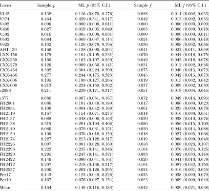
sample error rates across the 16 red fox microsatellite loci were, respectively, 0.17 allelic dropouts per hetero-zygote per locus (p) and 0.035 false alleles per genotype per locus (f). The mean ML estimates were 0.16 and 0.018, respectively. For the 17 Ethiopian wolf micro-satellites, the mean sample error rates werep¼0.16 and
f¼0.049, while the mean ML estimates were 0.14 and 0.040, respectively. Thus, with the exception of under-estimating f in the fox genotypes, the ML method performed well in estimating the mean cross-locus error rates.
For individual loci, ML estimates ofpwere generally close to the sample error rates, although they tended to be slightly underestimated in both the fox (mean bias
12%) and wolf data sets (mean bias13%; Table 2, Figure 5). The bias in the fox data was of opposite sign to the value predicted by the heterozygote deficit (3%), suggesting that other factors have greater influence on bias in real data. Almost half of the bias in analyzing the wolf data set was due to two loci, Pez19 and FH2137. Underestimation ofpin FH2137 was explained by a lack of information in the data due to a low He of 0.30 (sample p ¼0.087, ML p ¼0.048), while short allele dominance severely affected locus Pez19 (sample p¼
0.17, ML p¼0.076), although it was not a significant factor in any other locus. The linear relationship between sample and MLpwas tight ([MLp]¼0.973
[sample p]0.0097,R2¼0.94), and the slope of the line was not significantly different from 1 (t31¼0.69,
P¼0.50).
Figure4.—The effect of heterozygote deficiency, gauged by the inbreeding coefficientFIS, on relative bias in estimating
allelic dropout rate (e1) averaged over 5000 simulated data
sets. Low (e1 ¼ 0.01, solid line) and intermediate (e1 ¼
0.09, dashed line) allelic dropout rates were estimated at three false allele error rates (d, e2¼ 0.0015;s,e2 ¼0.04; ;, e2¼0.08). Other parameter values wereHe¼ 0.85 and
Bias in the locus-specific estimates of fof34% was considerably greater than in the estimates ofp, most notably in the fox duplicate genotypes where bias was
55%, much greater than the8% bias predicted due to heterozygote deficiency. Mean bias in the wolf data set was comparatively low at 17%. There were two principal reasons for underestimation of f in the fox data. First, the accumulation of errors in the most error-prone samples, combined with a tendency for the same rare false allele to recur across repeat genotypes, caused some errors to be hidden. For example, in locus V142 a 142/146 genotype was scored as 142/148.142/148
and a133/140genotype as142/142.142/142. In these two duplicate genotypes, four of the nine false alleles in the V142 genotypes went undetected. However, the
greatest cause of underestimation in the fox data, and to a lesser extent also in the wolf data, was the tendency of false alleles to occur preferentially in homozygotes, contrary to the third error model assumption. An excess of false alleles in homozygotes leading to extra ambig-uous duplicate genotypes (e.g.,AAread asAA.AB) will inflatepat the expense off.
Taking both data sets together, the scatter of the f
estimates was wider than that of thepestimates (Figure 5), possibly as a result of the comparatively small num-bers of false alleles in the duplicate genotypes (mean 10.8) compared with the number of allelic dropouts (mean 31.3). Nevertheless, the relationship between sample and MLfestimates was close ([MLp]¼0.763
[sample p] 0.0028, R2 ¼ 0.76). The slope of the TABLE 2
Analysis of the performance of the ML method in estimating allelic dropout and false allele error rates from real data
Locus Samplep MLp(95% C.I.) Samplef MLf(95% C.I.)
V142 0.138 0.116 (0.070, 0.176) 0.028 0.011 (0.002, 0.033) V374 0.464 0.429 (0.341, 0.517) 0.042 0.013 (0.002, 0.035) V402 0.000 0.000 (0.000, 0.011) 0.000 0.000 (0.000, 0.009) V468 0.027 0.019 (0.005, 0.049) 0.003 0.000 (0.000, 0.010) V502 0.016 0.005 (0.000, 0.031) 0.000 0.000 (0.000, 0.011) V602 0.084 0.069 (0.037, 0.114) 0.024 0.000 (0.000, 0.010) V622 0.132 0.126 (0.078, 0.196) 0.036 0.008 (0.002, 0.036) AHT-130 0.169 0.138 (0.090, 0.204) 0.041 0.027 (0.011, 0.059) CXX-156 0.175 0.161 (0.105, 0.231) 0.076 0.044 (0.018, 0.075) CXX-250 0.160 0.163 (0.107, 0.230) 0.049 0.045 (0.018, 0.078) CXX-279 0.120 0.089 (0.050, 0.141) 0.031 0.012 (0.002, 0.036) CXX-434 0.302 0.304 (0.224, 0.390) 0.075 0.040 (0.013, 0.073) CXX-466 0.277 0.244 (0.175, 0.323) 0.045 0.042 (0.015, 0.073) CXX-606 0.195 0.190 (0.127, 0.266) 0.019 0.015 (0.002, 0.042) CXX-608 0.213 0.224 (0.159, 0.302) 0.037 0.009 (0.002, 0.039) c2088 0.211 0.239 (0.171, 0.317) 0.051 0.019 (0.004, 0.045)
c377 0.086 0.087 (0.031, 0.167) 0.072 0.049 (0.016, 0.095) FH2001 0.086 0.101 (0.048, 0.180) 0.017 0.000 (0.000, 0.023) FH2054 0.100 0.094 (0.042, 0.169) 0.061 0.035 (0.009, 0.078) FH2119 0.167 0.154 (0.071, 0.275) 0.014 0.010 (0.000, 0.051) FH2137 0.088 0.048 (0.000, 0.163) 0.029 0.038 (0.010, 0.076) FH2138 0.315 0.294 (0.194, 0.408) 0.080 0.056 (0.015, 0.109) FH2140 0.086 0.079 (0.031, 0.151) 0.050 0.044 (0.014, 0.088) FH2159 0.100 0.070 (0.016, 0.159) 0.018 0.027 (0.005, 0.066) FH2174 0.227 0.213 (0.128, 0.317) 0.019 0.008 (0.000, 0.040) FH2226 0.097 0.081 (0.028, 0.160) 0.058 0.060 (0.023, 0.107) FH2293 0.222 0.235 (0.141, 0.346) 0.104 0.070 (0.024, 0.125) FH2320 0.295 0.247 (0.141, 0.371) 0.093 0.092 (0.033, 0.148) FH2422 0.140 0.090 (0.041, 0.161) 0.026 0.041 (0.013, 0.079) FH2472 0.207 0.218 (0.136, 0.317) 0.104 0.087 (0.032, 0.150) FH2537 0.200 0.202 (0.126, 0.295) 0.024 0.016 (0.001, 0.055) Pez17 0.143 0.123 (0.049, 0.228) 0.035 0.038 (0.009, 0.079) Pez19 0.167 0.076 (0.027, 0.154) 0.023 0.009 (0.000, 0.040)
Mean 0.164 0.149 (0.116, 0.183) 0.042 0.029 (0.021, 0.038)
Sample and ML estimates of error ratesp(allelic dropouts per heterozygote) andf(false alleles per genotype) in duplicate genotypes from 16 red fox and 17 Ethiopian wolf microsatellites (top and bottom, respectively). Confidence limits forpandfestimates (in parentheses) were converted from the horizontal and vertical di-mensions of the 95% confidence region fore1,e2(see Figure 1). Confidence limits for the mean are calculated
regression line differed significantly from 1 (t31¼3.1,
P ¼ 0.005), reflecting the greater bias in the f esti-mates compared with thepestimates.
DISCUSSION
The consequences of undetected microsatellite geno-typing errors can range from insignificant biases to out-right false conclusions (Gagneuxet al.1997; Abecasis
et al.2001; Hoffmanand Amos2005; Pompanonet al. 2005). Errors have become easier to correct or account for due to a combination of greater caution among re-searchers and the development of data analysis meth-ods that incorporate a single genotyping error rate. Error-tolerant microsatellite data analysis is more ac-curate when allelic dropout and false allele proba-bilities are estimated as separate parameters (Wang 2004; Hadfieldet al.2006; Kalinowskiet al.2006). The method described here estimates allelic dropout and false allele error rates without the limiting require-ment for reference data.
The results of the simulation analysis indicate that, even when reference samples are available, the ML method will generally estimate error rates more accu-rately than possible from an equivalent number of PCRs, provided that the data fit the assumptions of the error model reasonably closely. This counterintuitive result is explained by the fact that the cost in added uncertainty due to both duplicates being error prone is outweighed by the reduction in sampling error caused by doubling the sample size of error-prone genotypes. The simulation analysis also suggested that the ML method is generally robust to modest violations of the assumptions of the underlying error model, although
varying sample quality does lead to underestimation of e1 and e2 at high e1. This bias occurs because
co-incidence of dropouts and false alleles leads to under-counting of errors in the most error-prone simulated duplicate genotypes: the number of uncounted double dropouts will be higher than expected, as will the number of false alleles that are hidden by dropouts. Error esti-mates should therefore be used with caution when both high dropout levels and highly skewed sample quality are suspected. One way of mitigating this problem would be to identify and eliminate the most error-prone samples by comparing data quality across loci.
To what extent does the assumption of Hardy– Weinberg equilibrium (HWE) limit the use of our method? The standard error of the mean error rates es-timated from simulated data was unaffected by highFIS. Bias was also tolerably low except in rare cases wheree1
is very low relative toe2. Chesser(1991, Figure 2 therein)
has shown theoretically that under most realistic circum-stancesFISshould not be.0.1, although no cross-taxon survey of FIS-values exists to test this prediction. How-ever, empirical estimates show that HWE is a reasonable assumption within populations of humans (Altshuler
et al. 2005), which form the basis of most studies that consider genotyping error (Pompanonet al.2005). The 12 pedigree studies of bird and mammal populations reviewed by Slateet al.(2004) revealed predominantly low levels ofFIT(quoted asf; mean 0.042, range 0.002– 0.103), and even these low values probably represent publication bias in favor of highFIT. Assuming thatFST
is zero or positive, FITwill set an upper bound onFIS
because 1FIT¼(1FIS)(1FST) (Wright1951), in-dicating that in many if not most vertebrate popula-tions HWE will not be an unduly restrictive assumption,
provided that the populations are correctly defined and no Wahlund effect is present. It is important to note that a high pedigree inbreeding coefficient (equivalent to Wright’s FIT), which indicates shared coancestry within a population (Kellerand Waller2002), does not necessarily imply heterozygote deficiency and there-fore would not in itself affect our method. Very large heterozygote deficits that would invalidate our method are likely to be more common in nonvertebrate taxa as a result of greater mating system diversity (e.g., self-fertility in plants and molluscs). However, provided that prior information on mating system and genetic structure is used judiciously, our method should be applicable to a large majority of microsatellite geno-typing studies, particularly considering the large bias toward humans and wild vertebrates in microsatellite studies.
When presented with real data, the ML method per-formed well in approximating the sample error rates of both allelic dropout and false alleles, with the excep-tion that it systematically underestimated the false allele rate in the fox data set. This result suggests that in some data sets at least there will be significant deviation from the assumptions of the error model. The major cause of underestimation, the tendency of false alleles to prefer-entially affect homozygotes, is probably a consequence of the fact that artifactual alleles, as opposed to scoring and data entry errors, form a much higher proportion of false alleles in data derived from low-quality DNA, such as the genotypes from autoclaved fox teeth and wolf feces analyzed here (Bradleyand Vigilant2002; Pompanonet al.2005). Whereas a scoring or data entry error in a heterozygote will cause an existing allele to be miscalled, an artifactual allele will create a third allele, with two possible consequences: the genotype will be deleted (i.e., recorded as missing data), or two of the three alleles will be recorded as the genotype, which will include the artifactual allele with at most two-thirds probability. Either result will bias false alleles toward homozygotes when artifactual alleles are frequent, raising the possibility that there are two false allele error rates in error-rich data, one specific to homozygotes and the other to heterozygotes. However, in more typical studies when high-quality DNA is available, this bias should be greatly reduced if not absent. Hoffmanand Amos(2005) found that in low-error data (0.0038 errors per single-locus genotype), only 7% of errors that our model would class as false alleles were due to artifacts, the remainder being either due to scoring or data input errors (89%) or of unknown origin (4%). Scoring and data input errors should not affect homozygotes pref-erentially and may even show a bias toward heterozy-gotes, which present double the opportunities for error. The other significant source of underestimation of both error rates in the simulated and real data, clustering of errors in low-quality samples, should also be much less prevalent when template DNA is of high quality,
prin-cipally because the probability of duplicates hit by two errors is the square of the per-genotype error rate.
It remains to be seen how well our error model will fit a wider range of microsatellite data sets with differing frequencies and patterns of errors. The error model could easily be adapted to specific circumstances by adjusting the expected frequencies of the seven dupli-cate genotype dupli-categories. Our intention here was to provide a general model that enables parameters to be estimated for use in analyses that incorporate similar error models (e.g., Wang2004; Hadfieldet al.2006).
Where such error-tolerant analyses are unavailable, error rate estimates are nevertheless helpful in eval-uating the robustness of analyses to genotyping error. In the event that an analysis method is judged unac-ceptably error sensitive, error rates can be reduced by multiple genotyping. A simulation-based method is available to monitor the error sensitivity of a number of population parameter estimates (allele frequencies,
He,Ho, probability of identity, and census size) and to select the minimum number of repeat genotypes re-quired to reduce the impact of errors to acceptable levels (Valie` reet al.2002).
assuming zero error estimates is never advisable. An alternative if somewhat arbitrary approach is to use upper confidence limits rather than ML estimates. Although these values will generally be overestimates, particularly when sample size is small, it may often be safer to over-estimate than to underover-estimate error rates whether error rate estimates are greater than zero or not. Indeed, when there is ample information in the data, gross overesti-mates can allow greater accuracy in reconstruction of full-sib families than relatively modest underestimates (Figure 4 of Wang 2004). Morrissey and Wilson (2005) reached the opposite conclusion on the basis of parentage analysis of simulated and real data using the method of Marshallet al. (1998). Under certain circumstances (mother unknown, few marker loci, skewed allele frequencies, and a requirement of 95% confi-dence in correct assignment) there was a benefit in underestimating a 1% error rate. Not surprisingly, this benefit rapidly became a cost with increasing numbers of loci. In this study genotyping error was modeled as a single cross-locus quantity, so it is not clear to what extent, if at all, this result applies to methods that model allelic dropout and false allele error rates separately.
In practice, the level of imprecision that can be tol-erated in the error rate estimates could be assessed during the planning stage of a study by analyzing sim-ulated data. The robustness of the analysis to inaccu-racy in the error estimates could also be gauged after the data have been generated by repeating the analysis using a range of error estimates based on the confi-dence regions. Once the desired level of precision in the error estimates is known, how many duplicate samples will be needed to achieve it? As we have shown using simulations, for each locus this number will depend on the expected heterozygosity, which will usually be known, and error rates, for which plausible ranges can usually be predicted. The effect of varying sample size and error rates on error estimate precision can be ex-plored using simulations in Pedant.
In conclusion, we have developed a method for es-timating locus-specific rates, with confidence regions, of allelic dropout and false allele genotypic error from duplicate microsatellite genotypes without the require-ment for reference data. These error estimates can provide input for microsatellite data analysis methods that handle allelic dropout and false allele error rates separately. The method described here is implemented in a computer program, Pedant, which also uses sim-ulations to perform power analyses. The source code and executable are freely available for download from http://www.stats.gla.ac.uk/paulj/pedant.html.
We thank Tanita Casci, Ian Ford, Jarrod Hadfield, Lukas Keller, Barbara Mable, Graeme Ruxton, Peter Wandeler, and Jinliang Wang for discussion and advice and two anonymous reviewers for constructive comments on the manuscript. We are particularly grateful to Peter Wandeler and Deborah Randall for sharing their data. P.C.D.J. was supported by a Leverhulme Trust research project grant.
LITERATURE CITED
Abecasis, G. R., S. S. Chernyand L. R. Cardon, 2001 The impact
of genotyping error on family-based analysis of quantitative traits. Eur. J. Hum. Genet.9:130–134.
Altshuler, D., L. D. Brooks, A. Chakravarti, F. S. Collins, M. J.
Daly et al., 2005 A haplotype map of the human genome.
Nature437:1299–1320.
Bonin, A., E. Bellemain, P. Bronken Eidesen, F. Pompanon, C.
Brochmanet al., 2004 How to track and assess genotyping
er-rors in population genetics studies. Mol. Ecol.13:3261–3273.
Bradley, B. J., and L. Vigilant, 2002 False alleles derived from
mi-crobial DNA pose a potential source of error in microsatellite genotyping of DNA from faeces. Mol. Ecol. Notes2:602–605. Breen, M., S. Jouquand, C. Renier, C. S. Mellersh, C. Hitteet al.,
2001 Chromosome-specific single-locus FISH probes allow an-chorage of an 1800-marker integrated radiation-hybrid/linkage map of the domestic dog genome to all chromosomes. J. Genome Res.11:1784–1795.
Broquet, T., and E. Petit, 2004 Quantifying genotyping errors in
noninvasive population genetics. Mol. Ecol.13:3601–3608.
Chesser, R. K., 1991 Influence of gene flow and breeding tactics on
gene diversity within populations. Genetics129:573–583. Creel, S., G. Spong, J. L. Sands, J. Rotella, J. Zeigleet al., 2003
Pop-ulation size estimation in Yellowstone wolves with error-prone noninvasive microsatellite genotypes. Mol. Ecol.12:2003–2009. Ewen, K. R., M. Bahlo, S. A. Treloar, D. F. Levinson, B. Mowry
et al., 2000 Identification and analysis of error types in high-throughput genotyping. Am. J. Hum. Genet.67:727–736.
Feakes, R., S. Sawcer, J. Chataway, F. Coraddu, S. Broadleyet al.,
1999 Exploring the dense mapping of a region of potential linkage in complex disease: an example in multiple sclerosis. Genet. Epidemiol.17:51–63.
Gagneux, P., C. Boeschand D. S. Woodruff, 1997 Microsatellite
scoring errors associated with noninvasive genotyping based on nuclear DNA amplified from shed hair. Mol. Ecol.6:861–868.
Gottelli, D., C. Sillero-Zubiri, G. D. Applebaum, M. S. Roy, D. J.
Girmanet al., 1994 Molecular genetics of the most endangered
canid: the Ethiopian wolf,Canis simensis.Mol. Ecol.3:301–312.
Hadfield, J. D., D. S. Richardsonand T. Burke, 2006 Towards
unbi-ased parentage assignment: combining genetic, behavioural and spatial data in a Bayesian framework. Mol. Ecol.15:3715–3730.
Hoffman, J. I., and W. Amos, 2005 Microsatellite genotyping errors:
detection approaches, common sources and consequences for paternal exclusion. Mol. Ecol.14:599–612.
Holmes, N. G., H. F. Dickens, H. L. Parker, M. M. Binns, C. S. Mellersh
et al., 1995 Eighteen canine microsatellites. Anim. Genet.26:132–133.
Jeffery, K. J., L. F. Keller, P. Arceseand M. W. Bruford, 2001 The
development of microsatellite loci in the song sparrow,
Melospiza melodia(Aves) and genotyping errors associated with good quality DNA. Mol. Ecol. Notes1:11–13.
Johnson, P. C. D., K. S. Llewellyn and W. Amos, 2000
Micro-satellite loci for studying clonal mixing, population structure and inbreeding in a social aphid,Pemphigus spyrothecae (Hemi-ptera: Pemphigidae). Mol. Ecol.9:1445–1446.
Johnson, P. C. D., L. M. I. Webster, A. Adam, R. Buckland, D. A.
Dawsonet al., 2006 Abundant variation in microsatellites of
the parasitic nematodeTrichostrongylus tenuisand linkage to a tan-dem repeat. Mol. Biochem. Parasitol.148:210–218.
Jones, A. G., and W. R. Ardren, 2003 Methods of parentage analysis
in natural populations. Mol. Ecol.12:2511–2523.
Kalinowski, S. T., M. L. Taperand S. Creel, 2006 Using DNA
from non-invasive samples to census populations: an evidential approach tolerant of genotyping errors. Conserv. Genet.7:319–329.
Keller, L. F., and D. M. Waller, 2002 Inbreeding effects in wild
populations. Trends Ecol. Evol.17:230–241.
Kirkpatrick, S., C. D. Gelattand M. P. Vecchi, 1983 Optimization
by simulated annealing. Science220:671–680.
Legendre, P., and L. Legendre, 1998 Numerical Ecology.Elsevier,
Amsterdam.
Marshall, T. C., J. Slate, L. E. B. Kruukand J. M. Pemberton,
1998 Statistical confidence for likelihood-based paternity infer-ence in natural populations. Mol. Ecol.7:639–655.
Miller, C. R., P. Joyce and L. P. Waits, 2002 Assessing allelic
Morrissey, M. B., and A. J. Wilson, 2005 The potential costs of
ac-counting for genotyping errors in molecular parentage analyses. Mol. Ecol.14:4111–4121.
Navidi, W., N. Arnheimand M. S. Waterman, 1992 A
multiple-tubes approach for accurate genotyping of very small DNA sam-ples by using PCR: statistical considerations. Am. J. Hum. Genet.
50:347–359.
Neff, M. W., K. W. Broman, C. S. Mellersh, K. Ray, G. M. Acland
et al., 1999 A second-generation genetic linkage map of the do-mestic dog,Canis familiaris.Genetics151:803–820.
Nei, M., and A. K. Roychoudhury, 1974 Sampling variances of
het-erozygosity and genetic distance. Genetics76:379–390.
Ostrander, E. A., G. F. Spragueand J. Rine, 1993 Identification
and characterization of dinucleotide repeat (CA)n markers for genetic mapping in dog. Genomics16:207–213.
Ostrander, E. A., F. A. Mapa, M. Yeeand J. Rine, 1995 One
hun-dred and one new simple sequence repeat-based markers for the canine genome. Mamm. Genome6:192–195.
Paetkau, D., 2003 An empirical exploration of data quality in
DNA-based population inventories. Mol. Ecol.12:1375–1387.
Piggott, M. P., E. Bellemain, P. Taberlet and A. C. Taylor,
2004 A multiplex pre-amplification method that significantly improves microsatellite amplification and error rates for faecal DNA in limiting conditions. Conserv. Genet.5:417–420.
Pompanon, F., A. Bonin, E. Bellemainand P. Taberlet, 2005
Geno-typing errors: causes, consequences and solutions. Nat. Rev. Genet.
6:847–859.
Randall, D. A., 2006 Determinants of genetic variation in
Ethio-pian wolves. Ph.D. Thesis, Department of Zoology, University of Oxford, Oxford.
SanCristobal, M., and C. Chevalet, 1997 Error tolerant parent
identification from a finite set of individuals. Genet. Res. 70:
53–62.
Sieberts, S. K., E. M. Wijsmanand E. A. Thompson, 2002
Rela-tionship inference from trios of individuals, in the presence of typing error. Am. J. Hum. Genet.70:170–180.
Slate, J., P. David, K. G. Dodds, B. A. Veenvliet, B. C. Glasset al.,
2004 Understanding the relationship between the inbreeding coefficient and multilocus heterozygosity: theoretical expecta-tions and empirical data. Heredity93:255–265.
Smith, K. L., S. C. Alberts, M. K. Bayes, M. W. Bruford, J. Altmann
et al., 2000 Cross-species amplification, non-invasive genotyp-ing, and non-Mendelian inheritance of human STRPs in savan-nah baboons. Am. J. Primatol.51:219–227.
Sobel, E., J. C. Pappand K. Lange, 2002 Detection and integration
of genotyping errors in statistical genetics. Am. J. Hum. Genet.
70:496–508.
Taberlet, P., S. Griffin, B. Goossens, S. Questiau, V. Manceau
et al., 1996 Reliable genotyping of samples with very low DNA quantities using PCR. Nucleic Acids Res.24:3189–3194.
Taberlet, P., L. P. Waitsand G. Luikart, 1999 Noninvasive genetic
sampling: look before you leap. Trends Ecol. Evol.14:323–327. Valie` re, N., P. Berthier, D. Mouchirod and D. Pontier,
2002 GEMINI: software for testing the effects of genotyping errors and multitubes approach for individual identification. Mol. Ecol. Notes2:83–86.
Waits, J. L., and P. L. Leberg, 2000 Biases associated with
popula-tion estimapopula-tion using molecular tagging. Anim. Conserv.3:191–199.
Walters, K., 2005 The effect of genotyping error in sib-pair
ge-nomewide linkage scans depends crucially upon the method of analysis. J. Hum. Genet.50:329–337.
Wandeler, P., 2004 Spatial and temporal population genetics of
Swiss red foxes (Vulpes vulpes) following a rabies epizootic. Ph.D. Thesis, School of Biosciences, University of Cardiff, Cardiff, UK.
Wandeler, P., and S. M. Funk, 2006 Short microsatellite DNA
mark-ers for the red fox (Vulpes vulpes). Mol. Ecol. Notes6:98–100.
Wandeler, P., S. Smith, P. A. Morin, R. A. Pettiforand S. M. Funk,
2003 Patterns of nuclear DNA degeneration over time—a case study in historic teeth samples. Mol. Ecol.12:1087–1093. Wang, J., 2004 Sibship reconstruction from genetic data with typing
errors. Genetics166:1963–1979.
Wattier, R., C. R. Engel, P. Saumitou-Lapradeand M. Valero,
1998 Short allele dominance as a source of heterozygote defi-ciency at microsatellite loci: experimental evidence at the dinu-cleotide locus Gv1CT inGracilaria gracilis(Rhodophyta). Mol. Ecol.7:1569–1573.
Wright, S., 1951 The genetical structure of populations. Ann.
Eugen.15:323–354.
Communicating editor: D. Charlesworth
APPENDIX
Likelihood calculation:To simplify the presentation of the equations for the expected category frequencies, we use
per-genotype rather than per-allele error probabilities. For a single genotype at a single locus, we define the probability of no dropouts asp0¼(1e1)2and the probability of one dropout in a given allele asp1¼e1(1e1). Double dropouts are not counted. Similarly, the per-genotype probabilities for false alleles aref0¼(1e2)2,f1¼e2(1e2), andf2¼e2
2 .
The expected frequency (P1,2,. . .,7) of each repeat genotype category can be expressed by summing the probabilities of
all the ways in which a repeat genotype can contribute to that category. For example, one way for an observed duplicate genotype to enter category 3 (AA.AB) is via the occurrence in a homozygote of no dropouts and one false allele in any of the four alleles, with probability (1He)4p2
0 f0f1. If all possible states are considered, there are 512 ways of entering
the seven categories or the double-dropout category. This number is reduced to 198 by not counting double dropouts and ignoring replicates with more than two false allele errors. The expected frequencies of categories 1–7 are
P1¼PðAA:AAjHe;e1;e2Þ ¼ ð1HeÞðp2
0 f 2
0 14p0p1f 2
0 14p0p1f0f114p 2 1 f
2 0 18p
2
1 f0f114p 2 1 f
2
1 Þ1Heð2p 2 1 f
2 0 14p
2
1 f0f112p 2 1 f
2 1 Þ P2¼PðAB:ABjHe;e1;e2Þ ¼Heðp02f02Þ
P3¼PðAA:ABjHe;e1;e2Þ ¼ ð1HeÞð4p02f0f118p0p1f0f118p0p1f12Þ1Heð4p0p1f0218p0p1f0f114p0p1f12Þ P4¼PðAA:BBjHe;e1;e2Þ
¼ ð1HeÞð4p0p1f0f114p0p1f0f218p12f0f118p12f0f2112p12f12Þ1Heð2p12f02112p12f0f1114p12f12112p12f0f2Þ P5¼PðAB:ACjHe;e1;e2Þ ¼ ð1HeÞð4p02f
2
1 Þ1Heð4p 2
0 f0f112p 2 0 f
2 1 Þ
Because double dropouts are not counted, these probabilities must be normalized to sum to one, giving the expected frequency of categoryi,
Fi¼
Pi P7
i¼1Pi
:
The data consist of the seven observed category counts, X1,. . ., X7, which sum to n, the number of duplicated genotypes. The likelihood,L, of the data given the expected heterozygosityHeand error ratese1ande2is
PðXjHe;e1;e2Þ ¼
n!
X1!X2!;. . .X7!F X1
1 F
X2
2 ;. . .F
X7
7 :
Maximum-likelihood search algorithm: The maximum-likelihood search begins at a random point on the
like-lihood surface and proceeds by a simulated annealing procedure (Kirkpatricket al.1983). New error coordinates are proposed by randomly adding or subtracting a step of sizeSto or from each error rate. The likelihood of the new coordinates (Lnew) is compared with that of the old (Lold). Uphill steps (Lnew . Lold) are always accepted while downhill steps are accepted with probability (Lnew/Lold)1/T, where T is the annealing temperature, allowing the
search to escape from a local maximum. Downhill steps are more likely to be taken when the proposed drop in likelihood is modest andTis high. BecauseTdecreases as the search continues, the probability of a downhill step decreases toward the end of the search.Tbegins the search at a value of 1000 and decreases multiplicatively every iteration by a factor of 1011/i
, whereiis the number of search iterations, so thatTapproaches 108toward the end of the search regardless of i. During the last 10% of the search only uphill steps are permitted. Like T, S
decreases exponentially throughout the search, from a maximum of 0.1 to a minimum of 107. The initial and final values ofTandSand the shapes of their declines are independent of i, with the practical result that regardless of
iapproximately the first half of the search is spent searching widely across the likelihood surface for a peak to settle on and the remainder is spent refining the error estimates on that peak. The search jumps to the last 1000 iterations if the likelihood of accepted steps increases by,1% for 1000 consecutive iterations.
An additional search procedure further reduces the probability of the search ending on a local maximum. Afteri
iterations have been completed, the maximum likelihood recorded throughout the search is compared with the final likelihood. If the former is higher, the final coordinates must represent a local maximum, so the search returns to the likelier recorded coordinates, which must be located either on a higher local maximum or on the global maximum. Finally, a further 1000 optimization iterations are completed, again with exponentially decreasingSbut with only uphill steps being allowed.
We tested the search algorithm by analyzing artificial data sets that produce bimodal likelihood surfaces with a narrow global maximum and a broad (and therefore more easily located) local maximum. The global maximum was located within 20,000 iterations in 100/100 trials except when the difference in likelihood between the two peaks was low (likelihood ratio,2.2). In these cases 500,000 iterations were required to locate the global maximum in 82/100 trials.
Simulation of sampling error inHe:The point estimate ofHeused to calculate the expected frequencies is subject
to sampling error, which was incorporated into the simulated estimate ofHeused in estimating the error rates. EstimatedHewas simulated as a normally distributed random variable with meanHeand standard deviations. Because
sis a function of both allele frequency distribution and the number of genotypes from whichHewas calculated,nH
(Neiand Roychoudhury1974), simulation ofswas simplified by assuming a single allele-frequency distribution, the expected frequencies determined from the broken-stick distribution (Legendreand Legendre1998). Broken-stick frequencies can be used to provide a simple means of simulating realistic microsatellite allele frequencies (Kalinowskiet al.2006). Given broken-stick expected frequencies, for anynHbothHeandsare discrete functions of the number of alleles. We derived a close approximation ofs,
sa¼ð1HeÞðffiffiffiffiffiffiffiffiffiffiffiffi113HeÞ 20nH
p ;
by fitting a curve to discrete values ofsacross a realistic range ofHe(0.38–0.95, which corresponds to 2–29 alleles) and
nH(50–20,000). The approximationsaaccounts for 98.1% of the variation insatnH¼50 and.99.5% atnH$100.
Although all microsatellite allele-frequency distributions will deviate from broken-stick expected frequencies to some extent, comparison ofscalculated from data withsasimulated at the sameHeandnHfor data from 54 microsatellite
loci (Herange, 0.27–0.90;nHrange, 172–545) from aphids ( Johnsonet al.2000), nematodes ( Johnsonet al.2006),
Simulation of nonindependence of error rates among samples:We simulated the effect of variable sample quality by changing the probability distribution of ranked errors in the simulated data from uniform to a more realistic S shape. Multiplyinge1ande2in theith simulated duplicate genotype (i¼1, . . .,n) by
2
3 1cos p
i1
n1
2
1n2i
10n
skews the distribution of error probability so that 1.7% of error probability is distributed in the first 20% of the simulated genotypes and 48% in the last 20%. This expression was designed to mimic to the most severely skewed error distribution observed among the 16 fox microsatellite loci.
Conversion of per-allele to per-genotype error rates: For allelic dropout
p¼ 2e1 e111
;
where p is the per-heterozygote dropout rate for a single locus (Wang 2004). The conversion of e2 to f is less straightforward because, assuming that dropouts override false alleles, whene1is highfmust be adjusted to account for the proportion of false alleles that will be obscured by allelic dropout. Ife1is zero thenf¼1f0¼2e2e22, which
can be adjusted to allow for allelic dropout by multiplying by the probability of a false allele not dropping out (ignoring genotypes where both alleles are false), so that
f ¼ ð2e2e22Þ 1 e1 e111
;
which simplifies to
f ¼2e2e 2 2 e111