Protocols and Resources for New Generation Continuous Variable Quantum Key Distribution

(1)

Protocols and Resources for New Generation

Continuous Variable Quantum Key Distribution

Oliver Thearle

A thesis submitted for the degree of Doctorate of Philosophy in Engineering at

The Australian National University

August 2017

(2)

(3)

Declaration

This thesis is an account of research undertaken between February 2013 and August 2017 at The Research School of Engineering and The Department of Quantum Science, Research School of Physics and Engineering, The Australian National University, Can-berra, Australia.

Except where acknowledged in the customary manner, the material presented in this thesis is, to the best of my knowledge, original and has not been submitted in whole or part for a degree in any university.

Oliver Thearle August, 2017

(4)

iv

(5)

Acknowledgments

Firstly I would like acknowledge and thank my supervisory panel, Matt James, Jiri Janousek, Ping Koy Lam and Elanor Huntington and honorary member Syed Assad. You have all been very supportive of my research throughout my candidature. Your collective experience has provided me with valuable insight into research and quantum optics. Each one of you has greatly contributed towards the completion of this thesis. Thank you all so much for giving me the opportunity to complete a PhD.

Secondly I would like to thank the ANU quantum optics group and the whole of the department of quantum science for providing me a friendly environment to complete my thesis. There are far to many of you to list but through the many varied social activities the community of DQS has greatly contributed to enriching my time at ANU. My 1064 office and lab buddies, Jing-Yan Haw, Zhao Jie, Syed Assad, Mark Bradshaw, Thibault Michel, Hao Jeng and past members Seiji Armstrong, Helen Chrzanowski, Sara Hosseini, Jiao Geng, Alex Brieussel, thanks for putting up with me for so long even if I did tell some of you to be quiet for science from time to time. Thank you to Seiji, Jiri, Sara, Melanie Schünemann (Mraz) and many others for persevering with me through the Bell test experiment. After many years it is finally published. Thank you to Georgia Mansell for the random food, tea and for always making sure I went to the CGP Christmas party. Most importantly thank you to Amanda Haines (White) and Lynne Christians for the many Tim Tams and helping me navigate through the ANU bureaucracy.

My thanks to the climbing gang that I spent many weekends with talking and some-times climbing with. Geoff Campbell, Chris ’Bearded Chris’ Hunter Lean, Aaron Tran-tor, Giovanni Guccioni, Pierre Vernaz-Gris, Jess Eastman and the many others that I’ve climbed with, thanks for providing me with a fear of falling to distract me from my thesis over the years.

I would also like to thank my friends Joe, Carlie, Richard, Rachel, Peter, Vicki, Jon, Mel, Shaven Chris, Geoff, Ellen, Burgo and Emma. We’ve had many memorable mo-ments together while I’ve been a student watching you all progress through life. I’m hoping that now I’ve finished I can catch up to you all.

Lastly thank you to my immediate family for always being around to support and feed me. Especially to my mum who proof read my thesis in an amazingly short time.

As required by the “Commonwealth Scholarships Guidelines (Research) 2017” I ac-knowledge the support of the Australian Government through an Australian Government

(6)

vi

Research Training Program Scholarship.

(7)

Abstract

Quantum optics has been developing into a promising platform for future generation communications protocols. Much of this promise so far has come from the development of quantum key distribution (QKD). The majority of the development of QKD is done with discrete variables (DV), i.e. qubits with the underlying system of single photons. This is one interpretation of an optical field. Alternatively an optical field can be inter-preted as wave with the continuous variable (CV) observables of phase and amplitude. This interpretation comes with the advantage of access to high efficiency detection at room temperature and deterministic sources at the cost of susceptibility to noise in lossy channels.

This thesis presents an investigation of protocols and resources for the next generation of CV QKD protocols with two directions, the development of quantum state resources and the development of QKD protocols.This thesis starts with the details on the on going development of a low loss squeezed state resource using OPA for use in future communi-cation and estimation experiments. So far the OPA has produced 11dB of squeezing with 13dB predicted with reasonable improvements to losses and locking. Being able to per-form a Bell test with a CV Bell state is also key for future CV QKD protocols. Originally developed for DV systems the Bell test is a fundamental test of quantum mechanics. Here the first experimental demonstration of an optical CV bell test is presented. The experi-ment violated a CHSH Bell inequality with|B|= 2.31. This violation holds promise for being able to realise new device or source independent CV protocols.

The second half of this thesis proposes a channel parameter estimation protocol based on the method of moments and presents the results of a one side device independent CV QKD demonstration based on the family of Gaussian QKD protocols. The proposed channel parameter estimation protocol through the use of the method of moments is able to use information usually disregarded for estimation of an adversaries information. The result does not allow for an increase in range of a fully optimised protocol but can increase the key rate by an order of magnitude with high loss channels. Using a newly found entroptic uncertainty relation for CV tripartite states a new security proof was applied to the family of Gaussian CV QKD protocols. This resulted in the discovery of six new protocols with the special property of being one side device independent. Using the new security proof three of the protocols were demonstrated with a positive key rate.

(8)

(9)

Introduction

Quantum mechanics is a very counter intuitive interpretation of reality with its pre-dictions that go against how we experience the world. This is exemplified by the EPR paradox [1] which predicts a violation of the basic principle of local realism with non-local correlations. With this paradox in mind the famed Bell test [2] was developed and experimentally demonstrated using quantum optics to show that local realism is incorrect [3], albeit with some loopholes that could explain the violation. Recently four Bell test experiments have unequivocally demonstrated a violation of local realism by closing all of the major loopholes [4–7]. The original Bell test was formulated for discrete states and as such all four of these violations were made using single photons states. The study of single photons is part of a sub field of quantum optics known as Discrete Variable (DV) quantum optics. While DV is an interesting area this thesis explores the alternate sub field of Continuous Variable (CV) quantum optics [8] based on the equivalent interpretation of light as a wave. These two interpretations closely link the study of DV and CV quantum optics.

As well as fundamental research quantum optics is also providing a toolbox for a new generation of quantum based communication technologies with a few interesting exam-ples found in Ref. [9–11]. These new technologies will be crucial to realise a future where quantum mechanics will become ubiquitous for solving problems. One set of protocols that has found it way into commercial applications as a solution to the key distribution problem is quantum key distribution (QKD).

The key distribution problem can be described by a game where two parties, Alice and Bob, want to communicate a using a public channel controlled by an eavesdropper, Eve. Alice and Bob can communicate using encryption but the problem is how to distribute the encryption key without Eve intercepting it in a usable form. A common solution to this problem is to use a public key distribution protocol. A famous example of these protocols is the Diffie-Hellman key exchange protocol [12]. Using a combination of private and publicly exchanged information Alice and Bob can distil a shared secret. The finer details of this protocol are outside of the scope of this thesis but the security of the publicly exchanged information relies on the difficult problem of integer factorisation. This is an easy task for small numbers but it becomes exponentially harder for large numbers. In computer science it is believed to be an NP-intermediate problem which is presumed to

(14)

2 CONTENTS

be a hard class of problems. While it is currently hard to solve on a classical computer this and other difficult problems might not be so hard on a quantum computer with Shor’s algorithm [13].

QKD uses physical principles to ensure security [14, 15]. A QKD protocol will have Alice generate a series of quantum states to send to Bob. Using the properties of quantum mechanics if Eve is listening any interaction she has with the transmitted states will create detectable errors between Alice and Bob. If the error rate is too high Alice and Bob can abort the protocol and try again or try to disassociate their shared secret from Eve’s intercepted information. The advantage of QKD is that its security will hold as long as the underlying physical principles do. With classical key distribution protocols Eve can record the transmitted bits. Then at a later date when the particular distribution protocol is broken she can use her records to decrypt any data sent in the past. The advent of general quantum computing has the potential to change how data is communicated and stored. There are efforts to investigate public encryption protocols that are hardened against the potential of quantum computing [16].

(15)

CONTENTS 3

Thesis Outline

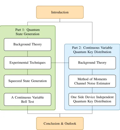
The structure of this thesis is illustrated in Fig. 1. The content has been split into two parts, Part 1: Quantum State Generation and Part 2: Continuous Variable Quantum Key Distri-bution. Each part starts with an overview of the material to provide some background and context. Part 1 covers the work that is more general to quantum mechanics and introduces the basic theory used here from the point of view of continuous variable quantum optics in Ch. 1. Building on this theory some of the experimental techninques used in this thesis are presented in Ch. 2. Following this the results from the development of a low intra-cavity loss OPA are presented in Ch. 3. Ch. 4 will present the results from the first optical CV Bell test. Part 2 covers the work relating specifically to CV QKD. It opens with an introduction to classical and quantum information theory. This chapter applies some of the ideas presented in Ch. 1 and concludes with an introduction to CV QKD. Ch. 6 details the application of the method of moments estimator to CV QKD to estimate the channel noise. The one-sided-device-independent CV QKD protocols with their demonstrations are given in Ch. 7. The thesis is concluded in Ch. 8 with a summary of the key results and a perspective on where the field of CV QKD is headed.

Publications

1. O. Thearle, S. M. Assad, T. Symul, “Estimation of output-channel noise for continuous-variable quantum key distribution,”Physical Review A,93, 042343 (2016).

2. N. Walk, S. Hosseini, J. Geng, O. Thearle, J. Y. Haw, S. Armstrong, S. M. Assad, J. Janousek, T. C. Ralph, T. Symul, H .M. Wiseman, and P. K. Lam, “Experimental demonstration of Gaussian protocols for one-sided device-independent quantum key distribution,”Optica,3, 634-642 (2016).

3. S. M. Assad, O. Thearle, and P. K. Lam “Maximizing device-independent random-ness from a Bell experiment by optimizing the measurement settings,” Physcial Review A,94, 012304 (2016).

(16)

4 CONTENTS

Part 1: Quantum State Generation

Part 2: Continuous Variable Quantum Key Distribution Introduction

Background Theory

Experimental Techniques

Squeezed State Generation

A Continuous Variable Bell Test

Background Theory

Method of Moments Channel Noise Estimator

One Side Device Independent Quantum Key Distribution

[image:16.595.75.484.180.623.2]

Conclusion & Outlook

(17)

Part I

Bell Tests and Quantum State

Generation

(18)

(19)

7

Overview

Quantum mechanics is not a very intuitive physical description of the world. Some of the more commonly known predictions by quantum mechanics such as Heisenberg’s uncer-tainty principle or entanglement do not align with our experience of the real world. For example it is common to observe local realism in our everyday experience. That is ob-jects around us appear to be in a real predetermined state and are only changed by local effects. However using quantum mechanics, local realism can be shown to not hold true for all systems. First with the thought experiment by Einstein, Podolsky and Rosen [1] where entanglement was first predicted and then more recently by a series of experiments disproving local realism [4–7]. As quantum mechanics is revealing a world unfamiliar to most, it is opening up opportunities to create some interesting technological advances in computing and communications. More often that not these developments in protocols and algorithms are either unrealisable with current abilities or restricted to a laboratory as the states required are difficult to create.

The following chapters will provide an introduction to the mathematics behind quan-tum mechanics and provide some description on creating and measuring quanquan-tum states. Ch. 1 will provide the basic maths and ideas for describing optical quantum states. This chapter will also contain a brief discussion on the experimental techniques used to create and measure quantum states. Ch. 3 will cover some work on creating highly squeezed quantum states which are hoped will be able to be used for quantum protocol demonstra-tions. The final chapter, Ch. 4 will discuss a continuous variable test of local realism.

(20)

(21)

Chapter 1

Background Theory

1.1 Quantum mechanics

This section will give a basic description of quantum mechanics for isolated and closed systems in a manner that will be helpful in understanding this thesis. The section is modelled from the postulates of quantum mechanics given in Ref. [13].

1.1.1 State space

In classical mechanics the representation of information is in bits. This unit of informa-tion is common and can be found in computing and communicainforma-tion theory. In practical systems the bit is encoded into two level systems such as a coin. A coin flip will put the coin into one of two states, either heads up or tails up. In quantum mechanics the analogue to a bit is a qubit which describes a two level system that is more complex as the system is allowed to be in a superposition between states. A quantum state can be described by a state vector which is a unit vector in a Hilbert space that describes the state space of the physical system of the quantum state. A Hilbert space is complex vector space with an inner product. For a qubit the state space is described by the orthonormal basis{|0⟩,|1⟩}. Here|i⟩ represents a vector in the state space using the ket notation. An arbitrary qubit state in this basis is written as,

|ϕ⟩=a|0⟩+b|1⟩ (1.1) The inner product is then given by⟨ϕ|ϕ⟩ = 1, where ⟨ϕ| is the vector dual of|ϕ⟩. The result of the inner product satisfies the requirement that the state vector be a unit vec-tor on the state space. In general an arbitrary pure state can be represented as a linear combination of the eigenstates.

(22)

10 Background Theory

1.1.2 Evolution

A closed quantum system can evolve through time with the evolution of a state at time t=t1,|ϕ⟩, related to the state att =t2,|ϕ′⟩by|ϕ′⟩=U|ϕ⟩whereU is a unitary operator,

that isU U†=IwhereU†is the Hermitian conjugate. The evolution can also be described by the Schrödinger equation,

iℏd|ϕ⟩

dt = ˆH|ϕ⟩, (1.2)

whereℏis Planck’s constant andHˆ is a Hermition operator, i.e. Hˆ = ˆH†, known as the Hamiltonian. There are two main interpretations of evolution, the Schrödinger picture and the Heisenberg picture. In the Schrödinger pictureHˆ is taken to evolve with time as the state vector does not. In the Heisenberg picture the state vector evolves with time and

ˆ

H does not. The Schrödinger picture is commonly used in to describe the evolution of discrete variable systems. For continuous variable systems the Heisenberg picture is used.

1.1.3 Measurement

The measurement of a quantum state can be described by a collection of measurement operators{Mˆm}wherem is the index of the measurement outcomes. For example

con-sider the qubit in Eq. (1.1) with the family of measurement operators Mˆ0 = |0⟩⟨0| and

ˆ

M1 = |1⟩⟨1|. The operatorMˆ0 will measure if|ϕ⟩ = |0⟩and similarlyMˆ1 will measure

if |ϕ⟩ = |1⟩. Though in quantum mechanics a state is not predefined so the measure-ment operators will have a probability of the measuremeasure-ment return a result 0or1. These probabilities are given by,

p(0) =⟨ϕ|Mˆ₀†Mˆ0|ϕ⟩=|a|2, (1.3)

p(1) =⟨ϕ|Mˆ₁†Mˆ1|ϕ⟩=|b|2. (1.4)

After a measurement is made the state will change depending on the result and become,

ˆ

Mm|ϕ⟩

√

⟨ϕ|Mˆm†,Mˆ|ϕ⟩

(1.5)

(23)

Quantum mechanics 11

Projective measurements

An equivalent description of the general measurement given above is the class of projec-tive measurements. A projecprojec-tive measurement is described by a Hermition operator, Mˆ, known as an observable. The observable can be decomposed into a linear combination of projectors,Pˆm, into the eigenspace ofMˆ,

ˆ

M =∑

m

mPˆm (1.6)

The outcomes of a projective measurements will correspond to the eigenvalue,m, ofMˆ. The probability of measuring the eigenvaluemis given by

p(m) = ⟨ϕ|Pˆm|ϕ⟩ (1.7)

After measurement givenmwas measured the state will become,

ˆ

Pm|ϕ⟩

√

p(m) (1.8)

The expected value for a projective measurement is easily calculated as,

E( ˆM) =⟨ϕ|Mˆ|ϕ⟩ (1.9) A common notation for the expected value is also ⟨Mˆ⟩. The variance of an observable follows as,

∆2( ˆM) =⟨Mˆ2⟩ − ⟨Mˆ⟩2 (1.10)

1.1.4 Composite systems

A composite system can be formed with individual component systems. The state space for a composite system is described by the tensor product of the component systems state spaces. A state vector in a composite system withncomponent systems is then described by|ϕ1⟩⊗|ϕ2⟩⊗. . .|ϕn⟩where|ϕi⟩is a state vector in the state space for theith component

system. The state vector is more commonly written as|ϕ1ϕ2. . . ϕn⟩. An operator acting

(24)

Entanglement

An important example of a composite system is an entangled state. For a composite sys-tem made up of syssys-tem A and syssys-tem B both described by the qubit state space. Consider the state,

1

√

2(|0A0B⟩+|1A1B⟩) (1.11)

This state is interesting because a measurement performed on system A will project the state of system B regardless of how far apart they are. Measurement of both states will reveal correlations that forgo local realism as a physical law. This topic is explored further in Sec. 1.2 and Ch. 4. Consider the set of measurement operators,Mˆm = ˆMmA⊗IˆBwhere

m={0,1},Mˆ_mAis defined in Sec. 1.1.3 andIˆBis the identity operator on the state space of system B. The projection of the state after measurement is given by,

ˆ

Mm|ψ⟩

√

⟨ψ|Mˆm†Mˆm|ψ⟩

=|mAmB⟩ (1.12)

System B has been projected to either |0⟩ or|1⟩ depending on the outcome on the mea-surement of system A.

1.1.5 Density operators

A more general way to describe the state of a quantum system is with a density operator. For a pure quantum system the density operator is given by ρˆ = |ϕ⟩⟨ϕ|. If the density operator can be written in this way it is said to be in a pure state. Additionally a state is pure if and only ifρˆ2 _{= ˆ}_{ρ. Conversely a mixed state is one that cannot be represented by}

a simple state vector but can be represented by an ensemble of pure states,

ˆ

ρ=∑

i

pi|ϕi⟩⟨ϕi|. (1.13)

The purity of a state can be measured by using the trace operator on the square of the density operator,tr( ˆρ2₎_{. The trace will give a value between}₁_/n_{and 1 with 1 representing}

a pure state and n being the dimension of the Hilbert space. A composite system can also be described by density operators for example a two mode state is represented as

ˆ

ρAB = |ϕAB⟩⟨ϕAB|. The partial trace operation can be used to remove a system form a

state,

ˆ

ρAB PT

(25)

Bell Tests 13

For this thesis density operators are not used in any meaningful way other than a conve-nient way to refer to a quantum state and in particular mixed states. A more complete description is given in Ref. [13].

1.2 Bell Tests

The Bell test is a fundamental demonstration of quantum mechanics. It is made up of a family of inequalities that test the hypothesis of local realism [22]. A violation of a Bell inequality by two spatially separated parties will demonstrate non local correlations between them which is an indication of quantum entanglement. The original idea of en-tanglement is know as the EPR Paradox [1]. The Authors of the EPR paradox conducted a thought experiment where two separated particles, A and B, that have previously inter-acted could from the measurement of the position of A, infer the position of particle B beyond the quantum limit without it being disturbed. The conclusion was that quantum mechanics at the time did not provide a complete description of reality. It was suggested that a hidden variable could be used to explain the paradox. John Bell explored the para-dox and came up with a theorem that any local hidden variable model would be violated by the predictions of quantum mechanics [2]. To test this theorem many Bell inequalties have been proposed to bound results from a local hidden variable description of experi-mental results [22]. The most famous of them is the CHSH Bell inequality [23],

(26)

Bob

Alice

MB

M_B′ MA

M_A′

±1 ±1

Figure 1.1: A source distributes a Bell state to Alice and Bob. Alice and Bob each have their own measurement apparatus that can perform one of two measurements. Comparing their measurements they can violate Eq. (1.15).

see that this quantity can only be±2. Now consider the mean value of this quantity, E(AB+AB′ +A′B′−A′B) = ∑

aa′bb′

p(a, a′, b, b′)(ab+ab′+a′b′−a′b) (1.16)

≤ ∑

aa′bb′

p(a, a′, b, b′)×2 (1.17)

= 2, (1.18)

Wherep(a, a′, b, b′)is the probability of the joint state being predetermined prior to mea-surement such that the result will be A = a, A = a′, B = b and B′ = b′. Using the linearity of the expected value the CHSH inequality in Eq. (1.15) can be derived.

Now consider the quantum state

|ϕ⟩= |01⟩ − |√ 10⟩

2 . (1.19)

Where the source distributes one mode to Alice and one to Bob. Using the observables,

ˆ

A=Z Bˆ = −Z√−X

2 (1.20)

ˆ

A′ =X Bˆ′ = Z√−X

2 , (1.21)

withX =|0⟩⟨0|+|1⟩⟨1|andZ =|0⟩⟨0| − |1⟩⟨1|. The expectation values are; E( ˆA,Bˆ) = √1

2, E( ˆA

′_,_Bˆ_{) =} _√1

2, E( ˆA

′_,_Bˆ′_{) =} _√1

2, E( ˆA, ˆ

B′) =−√1

2. (1.22)

Interestingly this gives,

(27)

Quantum states of light 15

A clear violation of the original inequality and a demonstration that with quantum me-chanics nature does not obey local-realism. The value of2√2is known as the Tsirelson’s bound. This is the largest possible violation with the CHSH inequality [24].

In the derivation above it was assumed that Alice and Bob could not interact and every measurement yielded a result. This of course is not realistic to experiments and there are several loopholes [22] that can cause a violation of a Bell inequality. The most obvious is communication between Alice and Bob which can easily violate Eq. (1.15). This is knowm as the locality loophole. For example every time Alice decides a measurement she could tell the Bob and cause fake Bell violations. This is easily solved in optics experiments where Alice and Bob are moved far enough apart that even with speed of light communication they cannot exchange any relevant information in the time it takes to perform a measurement [25]. Another common loophole comes from the measurement process. A realistic measurement will have some loss associated with it. This loss results in a third possible outcome from the measurement being a “no click” or 0. These “no clicks” can be discarded but there is a threshold of measurement efficiency below of which a violation can be faked [26]. This is known as the detection loophole or the fair sampling assumption as the recorded data has to be representative of the distributed state.

There have been a number of experiments dating back over 35 years [3] that have demonstrated a violation of a Bell inequality but only recently has it been possible to overcome both the detection and locality loopholes. There have so far been four experi-ment where a convincing violation has been produced [4–7]. Each of these experiexperi-ments employed high efficiency detection methods to address the detection loophole and care-ful analysis of the separation of Alice and Bob to address the locality loophole. Each measurement setting was also chosen at random using a mixture of several sources of random numbers including quantum random number generators (QRNG). These experi-ments have opened up the possibility for practical applications of Bell tests in quantum technology where one is faced with the question of verification of quantum devices. For quantum key distribution (QKD) and QRNGs, a violation of a Bell inequality can rule out any tampering of the quantum source or the measurement devices. This allows the user to achieve device independent (DI) protocols [18].

1.3 Quantum states of light

(28)

an optical field as,

ˆ

A(r, t) = ∑

k

(

ℏ

2ωkε0 ) [

ˆ

akuk(r)e−iωkt+ ˆa†ku∗k(r)e iωkt

]

(1.24)

where the vectorkis the propagation vector, ω is the angular frequency of the field,A0

is a complex vector potential orthogonal tok andaˆis the annihilation operator with its Hermitian conjugate,ˆa†the creation operator. The vector potential can be written as a sum of modes, i.e. subsystems, denoted by the subscript k. For each mode the annihilation and creation operators obey the following bosonic commutation relations, where uk are

vector mode functions corresponding to a mode with an angular frequencyωkandˆais the

annihilation operator with its Hermitian conjugate, aˆ† the creation operator. The vector mode functions define the direction of travel in the case of a traveling wave. The vector potential can be written as a sum of modes, i.e. subsystems, denoted by the subscript k. For each mode the annihilation and creation operators obey the following bosonic

commutation relations,

[ˆak,ˆa′k] = [ˆa†k,ˆa

′†

k] = 0 and [ˆak,ˆa

′†

k] =δkk′, (1.25)

From Eq. (1.24) the electric field operator,Eˆ(r, t), and the magnetic flux density operator,

B(r, t), can be found using,

ˆ

B=∇ ×Aˆ Eˆ =−∂

ˆ

A

∂t . (1.26)

This gives the electric field operator,

ˆ

E(r, t) = i∑

k

(

ℏωk

2ε0 )1

2 [

ˆ

akuk(r)e−iωkt)−ˆa†u∗(r)eiωt)

]

. (1.27)

The Hamiltonian of electromagnetic field can be found using,

ˆ

H = 1 2

∫

(ε0Eˆ(r, t)·Eˆ(r, t) +

1

µ0

ˆ

B(r, t)·Bˆ(r, t))dr (1.28)

=∑

k ℏωk

(

ˆ

a†_kˆak+

1 2

)

. (1.29)

(29)

modes that forms the basis for this thesis.

The significance of the number operator comes from it being observable with the discrete eigenstates,

ˆ

n|n⟩=n|n⟩, (1.30)

where n ∈ N. Two other observable operators are given by the natural analogue to the position and momentum, the amplitude, xˆ and phase pˆoperators. These operators are continuous variable observables and are defined in terms of the annihilation and creation operators,

ˆ

x=

√

ℏ

2ω(ˆa+ ˆa

†₎ _(1.31)

ˆ

p=i √

ℏω

2 (ˆa−ˆa

†₎_, _(1.32)

with the commutation relation,

[ˆx,pˆ] =iℏ. (1.33)

These can be considered in some sense to be the real and imaginary part of the annihilation operator [27]. The eigenstates for the quadrature variables are not physically realisable but are given by,

ˆ

x|x⟩=x|x⟩ and pˆ|p⟩=p|p⟩, (1.34) wherexandpare continuous variables. That isx∈ Randp∈ R[8, 28]. Makingxˆand

ˆ

p the continuous variable observables. Using the quadrature operators the electric field operator for a single mode can be rewritten in the form,

ˆ

E(r, t) =

(

ℏω

2ε )1

2

[ˆxsin(ωt−k·r)−pˆcos(ωt−k·r)], (1.35) wherekis the direction vector of the field. Unsurprisingly the quadrature operators act as the amplitude operators on the phase and quadrature components of the electric field. As the operatorsxˆandpˆare non commuting observables the Heisenberg uncertainty principle (HUP) places a lower bound on the uncertainty of these two operators with,

∆A∆B ≥ 1

2|⟨[A, B]⟩|. (1.36)

Using the phase and quadrature operators this becomes,

∆ˆx∆ˆp≥ 1

2|⟨[ˆx,pˆ]⟩|= 1

(30)

It is convenient for the remainder of this thesis to takeℏ = 2andω = 1to simplify the description of quantum states. This simplifies the uncertainty principle to,

∆ˆx∆ˆp≥1 (1.38)

1.3.1 The Fock states

While it is not widely used in this thesis it is useful to know about the Fock basis. The Fock basis is made up by the eigenstates of the number operator. A Fock state is represented by the vector |n⟩ wheren is the number of photons in an optical field. The Fock basis can be used to make optical qubits. The action of the creation, annihilation and number operators on a Fock state is,

ˆ

a†|n⟩=√n+ 1|n+ 1⟩, ˆa|n⟩=√n|n−1⟩ and nˆ|n⟩=n|n⟩. (1.39) The minimum energy state or vacuum state is denoted by|0⟩and is defined by

ˆ

a|0⟩= 0 (1.40)

with the expected value of this state given by,

⟨0|nˆ|0⟩= 0. (1.41) All Fock states are accessible from the repeated application of the creation operator. The Fock basis forms a complete basis and every state is orthogonal,

∞ ∑

n=0

|n⟩⟨n|= 1, ⟨n|m⟩=δmn. (1.42)

1.3.2 Coherent states

The coherent states are interesting as they are minimum uncertainty states and are the closest quantum states to a classical description of an optical field. The significance of these states is they are the natural state generated by a shot noise limited laser. These states are created by the application of the displacement operator on a vacuum state. The displacement operator is given by [19],

ˆ

(31)

A coherent state,|α⟩, can be written in the Fock basis as,

|α⟩= ˆD(α)|0⟩=e−|α|2/2∑

n

αn √

(n!)|n⟩. (1.44)

The coherent state has a indefinite number of photons. The probability distribution of the Fock states in a coherent state is Poisson,

P(n) = |⟨n|α⟩|2 = |α|

2n_e−|α|2

n! . (1.45)

Unlike Fock states coherent states are not orthogonal to each other and form an over complete basis,

⟨β|α⟩= exp

[

−1

2(|α|

2₊_|_β_|2_{) +}_αβ∗ ]

(1.46) The variance of the quadrature operators of a coherent state are given by,

∆ˆx= 1, ∆ˆp= 1 (1.47)

A coherent state is part of a family of minimum uncertainty states which achieve the HUP lower bound,

∆x∆p= 1 (1.48)

A simple illustration of a coherent state can be made by a ball and stick diagram as shown in Fig. 1.2 (a). The uncertainty of the state is represented by a ball of radius 1 which is centered atα=⟨xˆ+ipˆ⟩.

1.3.3 Squeezed states

A more general minimum uncertainty state is the squeezed state. The defining feature of a squeezed state is the unequal uncertainty in each quadrature. A squeezed coherent state can be generated first by applying the squeezing operator S(ε), with a squeezing parameter of ε = re2iϕ_{, and then the displacement operator to a vacuum state. The}

squeezing operator is given by [19],

ˆ

S(ε) = exp

(

1 2(ε

∗_ˆ_a2 ₋_ε_ˆ_a†2₎ )

. (1.49)

(32)

x (a)

p

α

1

x (b)

p

α

x′ p′

ϕ

e−r er

Figure 1.2: A ball and stick diagram. The uncertainty of a coherent state, (a), is repre-sented by a ball centered at 1₂⟨x+ip⟩=α. A squeezed state, (b), is scaled bye−r_{in the}

xquadrature ander in thepquadrature and rotated byϕ.

is also a minimum uncertainty state with the variance of the rotated quadrature given by

∆x=e−r ∆p=er. (1.50)

The photon number distribution for a squeezed state is given by,

P(n) =

(₁

2tanh(r) )n

n! cosh(r) exp

[

−|α|2− 1

2tanh(r)

(

(α∗)2eiϕ+α2e−iϕ)]|Hn(z)|2, (1.51)

where,

z = α+α

2_eiϕ_tanh(_r₎

√

2eiϕ_tanh(_r₎ , (1.52)

and |Hn(z)| is the nth Hermite polynomial. It is interesting to note that Hn(0) = 0

for odd values ofn. Operationally this means that squeezed vacuum states only contain even numbered Fock states. When the squeezing operator is used on a coherent state the probability distribution Eq. (1.51) will widen ifr <0or narrow ifr >0. For large values ofr the probability distribution will oscillate at higher photon numbers. The probability distribution for the case of lowris plotted in Fig. 1.3.

(33)

0 5 10 15 20 25 30 0

0.1 0.2

n

P

(

n

)

Figure 1.3: The photon number distribution for a coherent state (blue) with α = 3, a phase squeezed coherent state (yellow) withα = 3andr=−0.5, an amplitude squeezed coherent state (purple) withα = 3andr = 0.5and a vacuum squeezed state (red) with r= 2.5.

1.3.4 Thermal states

It is sometimes useful for the description of a quantum system to consider non-minimum uncertainty Gaussian states called thermal states. A thermal state is a mixed state that describes the field emitted by a black body. The density operator for this state using the Fock basis is given by [29],

ˆ

ρ= 1 1 + ¯n

∞ ∑

n=0 (

¯

n

1 + ¯n )n

|n⟩⟨n|, (1.53) wheren¯is the mean photon number in the field. The variance of the thermal states in the quadratures is given by∆2_x_{= ∆}2_p_{= 2¯}_n_{+ 1}_.

1.3.5 Two important unitary operators

The states discussed in Sec. 1.3 can be used in combination with other states using unitary operators. This section will cover two important operations for this thesis, the beam splitter operation and the phase shift operation.

Phase shift

The phase shift operator is parameterised by the variableθ. The transformation acting on fieldaˆinis simply,

ˆ

(34)

ain aout

bin

bout

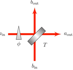
[image:34.595.204.360.96.244.2]

T ϕ

Figure 1.4: The optical fieldsˆain andˆbincombined on a beam splitter of transmission T.

Modeaˆinis shifted in phase byϕrelative toˆbin

The phase shift operator represents a rotation in the quadratures of an optical field,

ˆ

xθUˆPS(θ)ˆxUˆPS† (θ) = cos(θ)ˆx+ sin(θ)ˆp= ˆae−

iθ _{+ ˆ}_a†_eiθ _(1.55)

Beam splitter

A beam splitter is one of the more basic elements and most common of any optics ex-periment that is used to combine or split beams through a semitransparent surface with a transmission0 ≤ T ≤ 1and reflectivityR = 1−T. In quantum optics a beam splitter is always considered a four port device. A beam splitter can be combined with the phase shift operator to control which quadratures will interfere. Consider a beam splitter with a transmission ofT acting on two optical fieldsaˆinandˆbinthe transformation is given by,

[

ˆ

aout

ˆ

bout ]

=

[ _√

T √1−T

−√1−T √T ] [

e−iϕˆain

ˆ_b_in

]

, (1.56)

wheree−iϕis a phase shift acting on modeˆbin. A simple illustration of a beam splitter is

given in Fig. 1.4.

The beam splitter operator is significant in experimental modeling as it provides a way to model experiment losses. All experimental processes will experience some kind of loss. These include spatial mode matching, inefficient detection and scattering from optical components. The beam splitter operator can be used to model loss, and the coupling of a vacuum or a thermal state from the environment into the signal mode. In this thesis the second mode produced is considered destroyed, and the mode is traced out of the state. In the context of Fig. 1.4 if modeˆainis the signal then modeˆbinis the environment noise

(35)

Phase-space representation 23

1.3.6 Two mode squeezed states

The name two mode squeezed state gets comes from the property that the squeezing is now over two modes. Through this thesis they are commonly referred to as entangled states or EPR states. In this thesis an entangled state is generated from two squeezed vacuum states mixed in quadrature on a beam splitter withT = 0.5. The combination of the two squeezing operators and the beam splitter results in the two mode squeeze operator given by,

ˆ

S(G) = exp

(

G∗âAâB−Gaˆ†Aâ

†

B )

, (1.57)

whereG =re−iθ. This operator can be used to describe the generation of two entangled modes of different frequencies, ωA andωB. For this thesis the modes A and B will be

spatially separated. It is interesting to note that each mode in a two mode squeezed state has the quadrature variance∆2xˆ = ∆2pˆ= cosh(r). Meaning the modes individually are thermal states. The squeezing exists in the correlation between the two modes.

1.4 Phase-space representation

An alternative to describing a quantum state with a density operator is to use a Wigner function. The Wigner function is a quasiprobability distribution defined over a real sym-plectic space [28]. The Wigner function is outside the scope of this thesis but a compre-hensive description can be found in Ref. [30]. What is of interest here though is that the Wigner function can be described by the moments of the quantum state.

−2

0

2 −2 0

2 0

0.5

x

p

−2

0

2 −2 0

2 0

0.5

x

p

(a) (b)

Figure 1.5: Examples of a Wigner function for a coherent state, (a), and a squeezed state, (b), whereα= 1 +iandr= 0.5.

(36)

family of Gaussian states that can be completely described by their variance and mean in the phase and amplitude quadratures [29]. The covariance matrix and mean vector for a vacuum state is given by,

γ = [ 1 0 0 1 ] d= [ 0 0 ] . (1.58)

Here elementγ(1,1)andd1represent the variance and mean respectively of the state in the

xquadrature. Likewise for elementsγ(2,2) andd2in thepquadrature. Just as was shown

in Sec. 1.3 and Sec. 1.1.4 each of the minimum uncertainty states can be found by using an operator on the vacuum state. The covariance matrix for the single mode states is given by,

γ =

[

∆2_x ₀

0 ∆2_p ]

d=

[

⟨x⟩

⟨p⟩ ]

. (1.59)

The purity of a state described by a covariance matrix is given by ₂√1_γ [31].

1.4.1 Composite systems

Multiple modes in a state can be represented by a single covariance matrix and mean vector. ForN modes this would look like,

γ =

   

γ1 · · · C1,N

· · · . .. ... CN,1 · · · γN

  

 and d =

    d1 .. . dN   

, (1.60)

where each element γn andCn,m represents a 2×2 diagonal matrix, dn is a2 element

vector with n, m = {0,1, . . . , N}. The sub matrix Cn,m will represent the correlations

between modes n and m. A partial trace of a Gaussian composite system will remove an element from the covariance matrix and mean vector. Consider a partial trace on a bipartite system,ρABto trace out mode B. The covariance matrix will become,

γAB= [

γA C

C γB ]

PT

−→γA (1.61)

and the mean vector,

dAB= (dA, dB) PT

(37)

Phase-space representation 25

1.4.2 Gaussian operations

A Gaussian operator simply maps a Gaussian state to another Gaussian state. The corre-sponding operators for each of the operators given in Sec. 1.3 and Sec. 1.1.4 are given here.

Displacement operator

The displacement operator used to generate coherent states simply translates the mean of the state, dout = din +z, where z is the displacement in the x and p quadrature. The

covariance matrix under the displacement operator is invariant.

Symplectic transform

Any unitary operator US will have a corresponding symplectic operation S due to the

Stone-von Neumann theorem. A symplectic transformation applied with the mapping,

dout =Sdin γout =SγinST, (1.63)

whereSis2N ×2N matrix with real elements. The symplectic operation for the passive operations described in Sec. 1.3 are given below

Phase shift A phase shift of a mode by θ is simply a rotation between the quadratures. The symplectic operator for a single mode state is given by,

SPS(θ) = [

cos(θ) sin(θ)

−sin(θ) cos(θ)

]

. (1.64)

Beam splitter A beam splitter with transmission T acts on two modes with the sym-pletic operator,

SBS(T) =

[ _√

TI √1−TI

−√1−TI √TI ]

(1.65)

Squeezing operator The symplectic operator to squeeze a single mode state is given by,

SSq(r) =

[

e−r ₀

0 er

]

(1.66)

(38)

Two mode squeezed states The sympetic operators can be combined to create any Gaussian state. An important example for this thesis of this is generating an entangled state. As stated in Sec. 1.3.6 a two mode squeezed state can be created by combining two orthogonally squeezed states with a beam splitter. This gives the sympletic operator,

SBS(

1 2)S

A

Sq(r)S

B

Sq(−r) =

[

cosh(r)I sinh(r)σz

sinh(r)σz cosh(r)I

]

, (1.67)

where the super script represents the mode being acted on by the operator and,

σz =

[

1 0 0 −1

]

. (1.68)

1.4.3 CP Maps

Not all desired transformations are unitary and covered by symplectic transformations. The family of completely positive maps (CP map) can be used to perform irreversible operations such as loss and is defined by two matricesXandY applied to the covariance matrix and mean vector by,

γout =XγinXT +Y dout =Xdin (1.69)

Gaussian loss channel

A Gaussian loss channel can be modelled using a CP map with,

(39)

Chapter 2

Experimental Techniques

2.1 Detecting quantum states

In Ch. 1 the electric field was written as a discrete mode. To make sense of the detection of quantum states a continuum of frequency modes must be considered. A multimode system can be made by taking a sum of modes each with an angular frequency ωk and

propagation vectork. A continuum of modes can be made by considering the limit where the separation between the modes goes to 0. This creates new annihilation and creation operators which are related to the discrete operators by,

a→√∆ωa(ω) and a†→√∆ωa†(ω) (2.1) Understanding the continuum of modes is not essential to understand the work in this thesis. It is mentioned here to make the reader aware of the underlying description of sideband modes. For the work in this thesis, the modes discussed can be considered to be as described in Sec. 1.3. A rigorous description of this formalism for the continuum of modes is given Ref. [32, 33] and a more accessible description in Ref. [34]. The commutation relation for the new operators is now given by,

[a(ω), a†(ω′)] =δ(ω−ω′), (2.2) whereδ(ω−ω′)is the Dirac delta-function. The operatorsxˆ(ω)andpˆ(ω)are defined in a similar way to their discrete equivalents. The measurement of the observable operators are made relative to a carrier frequency, Ω, through the time varying field annihilation operator,

˜

a(t) =

∫ _∞

−Ω

ˆ

aΩ+ω(ω)eiωtdω, (2.3)

where ω is the separation from the carrier frequency and decoration, ˜, represents that the operator is in the time domain. The frequency domain annihilation operator can be

(40)

28 Experimental Techniques

extracted from the time domain using the Fourier transform, denoted byF, forω <Ω,

ˆ

a(ω) =F(˜a(t)) (2.4) Similarly the same relation exists for the quadrature operators to move from the time domain operator to the frequency domain. Measuring the modes relative to a carrier frequency is more widely known as the rotating wave approximation.

2.1.1 Phase and Amplitude modulations

Only phase modulations are used in this thesis however amplitude modulations can be de-scribed in a similar way. The phase modulations are used to make error signals and control phase and cavity lengths. They can also be used together with amplitude modulations as the displacement operator for side band modes. There are two different types of devices used for phase modulation in this thesis. For low modulation frequencies, typically be-low 100kHz, Piezo driven mirrors are used. For large modulation frequencies, typically above 1MHz, electro-optic modulators are used. These modulators apply an electric field to a crystal to change its refractive index. The modulation of an optical field in the time domain relative to the carrier frequency is given by,

˜

aPM = ˜aeiξcos(ωmt), (2.5)

where 0 ≥ ξ ≤ 1is the modulation depth andωm is the modulation frequency. A

mod-ulation ofωm will results in a number of harmonics being generated at integer multiples

ofωm with an amplitude that decays with the order of the harmonic. Assuming a small

modulation depth the phase modulated field can be approximated by,

˜

aPM ≈˜a (

1 +iξ

2e

iωmt₊_iξ

2e

−iωmt )

. (2.6)

The action of modulation is to move power from the carrier frequency,Ω,into the positive and negative sidebandsΩ±ωm. In the Fourier domain the modulation is given by,

ˆ

aPM =F(˜aPM) (2.7)

= ˆa+iξ

2aˆ(ω−ωm) +i

ξ

2ˆa(ω+ωm) (2.8)

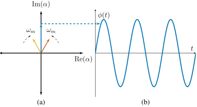
Phase modulation can be represented in a phasor diagram as illustrated relative to the carrier frequency in Fig. 2.1.

(41)

Detecting quantum states 29

t ϕ(t)

(b)

Re(α) Im(α)

ωm ωm

[image:41.595.151.480.94.273.2]

(a)

Figure 2.1: A phasor diagram, (a), showing the upper (red) and lower (yellow) sidebands rotating in opposite directions at a frequency ofωm relative to the carrier. The two

side-bands beat to create a phase modulation (blue) of the carrier, (b).

field relative to the carrier frequency is given by,

˜

aPM = ˜a(1 +ξcos(ωmt)). (2.9)

With the Fourier transform given by,

ˆ

aAM = ˆa+

ξ

2ˆa(ω−ωm) +

ξ

2ˆa(ω+ωm) (2.10)

2.1.2 Photodiode

A photodiode is a device that converts an optical field to a current using the photoelectric effect. The current produced is proportional to the photon number operator for the field [8, 19],

id(t)∝˜a†a.˜ (2.11)

To make sense of the diode current it is beneficial to consider the linearised decomposition of the annihilation and creation operators,

˜

(42)

made in Ref. [35]. With linearization of the operators the photodiode current becomes,

id(t)∝α2+αx.˜ (2.13)

Moving to the frequency domain and restricting the analysis to the frequency bands with no significant noise, the photocurrent can be written as upper and lower sidebands similar to the classical phase modulation. The upper,Ω +ωand lowerΩ−ωsidebands are given by,

id(ω) = i(ω) +i(−ω)∝α(ˆx(ω) + ˆx(−ω)) (2.14)

Experimentally the isolation of the sidebands in the detector current is made by using a combination of low and high pass electronic filters.

Photodetector

In an experiment the photodiode is used in a photodetector where the current is converted to a voltage using a transimpedance amplifier with some gaingd. A basic circuit of a

tran-simpedance amplifier can be found in App. A.1. The conversion of current to voltage can be done with a simple resister however for large gains this presents as a large impedance which reduces the signal to noise ratio. A transimpedance amplifier on the other hand presents as a low impedance load to the diode current through the use of an op amp for large gains [36].

2.1.3 Homodyne detection

The intensity can be easily measured using a single photodiode but to measure an arbitrary quadrature a homodyne detector is required. A homodyne detector works by interfering on a 50/50 beamsplitter a signal field, a, with a stronger local oscillator field,ˆ ˆaLO with

some relative phase θ between the two input fields. The strength of the local oscillator needs to be such thatαLO ≫α. Taking the difference between the two photocurrents as

depicted in Fig. 2.2 measures the quadraturexˆθ. The resulting measurement is amplified by the intensity of the local oscillator making it easier to measure weak quantum fluctua-tion in both quadratures. Using the linearisafluctua-tion of both fields the detected photocurrent is given by,

(43)

Detecting quantum states 31

The terms not containingαLOare approximately 0. Taking the Fourier transform ofidiﬀ(t)

the sideband mode can be written as,

idiﬀ(ω) =gDαLO(δx˜cos(θ) +δp˜sin(θ)) (2.16)

For the quadrature measurement to make any sense it needs to be normalized to shot noise which can be measured by blocking modea. For this thesis the normalization is such that the variance of the shot noise is one. For a state containing multiple correlated modes a

a

αLO

idif f(t)

50/50

[image:43.595.240.390.242.344.2]

–

Figure 2.2: A homodyne detector. The signal beam is interfered on a 50/50 BS. Both ports of the BS are measured and the photocurrents subtracted to getidif f.

homodyne measurement acts as a projective measurement to an infinitely squeezed state. In phase space the projection of the second mode of a bipartite state is given by the map [37],

γ_aout =γa−Cab(XγbX)M PCabT d out

a =Cab(XγbX)M P(m−db) +da, (2.17)

where X = diag(1,0,1,0), m = (X1,0) with X1 being the homodyne measurement

outcome andM P denotes the inverse on the range. The projection from the measurement of the pˆquadrature can be found by using X = diag(0,1,0,1) and m = (0, X1). A

homodyne is a destructive measurement so the original mode is traced out of the bipartite state.

Heterodyne detection

A homodyne detector can only measure one quadrature at a time. At the cost of 3dB loss two homodyne detectors can be combined using a 50/50 beam splitter to split the signal and measure both quadratures simultaneously as illustrated in Fig. 2.3. In phase space the projection is given by the map,

γ_aout =γa−Cab(γb+I)−1CabT, d out

a =

√

2Cab(γb+I)−1(m−dinb )+d in b )+d

in

(44)

wherem = (x1, p1)is the vector of the results from a heterodyne measurement on mode

ˆ_b

a

αLO

i+_{dif f}(t)

αLO

i−_{dif f}(t)

50/50 50/50

50/50

–

[image:44.595.168.400.138.311.2]

–

Figure 2.3: A heterodyne detector also know as a dual homodyne. The signal field is split on a 50/50 beam splitter and the resulting beams sent to homodyne detectors which are measuring orthogonal quadratures.

2.2 Optical resonators

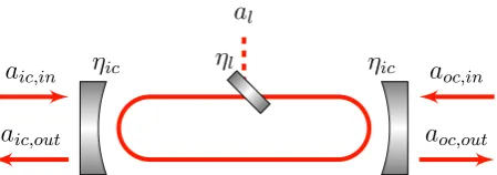
Optical resonators are used in this thesis to either define spatial and frequency modes by filtering an incident field or to increase non-linear effects through the resonance of the internal optical field. The most general optical resonators is a Fabry Pérot cavity. This cavity, illustrated in Fig. 2.4, consists of two mirrors, an input coupler (IC) and output coupler (OC), facing each other at some distance L. An optical field inside the cavity will reflect between the two mirrors with resonant modes constructively interfering. The resonant modes of the cavity have a wavelength that is a multiple of the cavity length. For a Fabry Pérot cavity this create standing waves in the cavity that constructively interfere with non-resonant wavelengths destructively interfering. Only the resonant modes will be transmitted through a cavity with the remaining modes reflected off the coupling mirrors. A cavity can be used to select specific frequency and spatial modes from an incident field by clever design of the geometry [38–40]. These properties allow a cavity to be used to filter the spatial and frequency modes from a laser.

As a closed system the internal field annihilation operator,a, will evolve in time ac-ˆ

cording to Heisenberg’s equation of motion,

˙˜

a= 1

(45)

Optical resonators 33 al aic,in aic,out aoc,in aoc,out

[image:45.595.204.429.92.171.2]

ηic ηl ηic

Figure 2.4: A model of an optical resonator with the fieldaic,incoupled through the IC

with transmissionηicand the counter propagating fieldaoc,incoupled through the OC with

transmissionηoc. The cavity loss is modelled as a beam splitter with transmissionηlwhich

couples the internal field to the environment.

In a closed system the Hamiltonian,Hrevis reversible. Open systems have non reversible

evolutions through lossy interactions with the surrounding environment. To account for the irreversible interactions extra terms can be added to Eq. (2.19) [41]. The modified equation of motion is know as the quantum Langevin equation and is given by,

˙˜

a(t) = 1

iℏ[˜a, Hrev]−[˜a,c˜

†_](_γ_˜_c₊√₂_γ˜_b_in₎₋₍_γ_˜_c†₊√₂_γ˜_b†

in)[˜a,˜c]. (2.20)

Here the operator ˜c is the system operator, ˜a, coupled to the environment ˜b and γ is the cavity decay. For a lossless passive resonator the Hamiltonian is given by Eq. (1.29) whereω= Ωis a resonant frequency. Using Eq. (1.29) with Eq. (2.20) gives the following equations of motion for an optical cavity coupled to the environment [21],

˙˜

a(t) =−(γ+i∆)˜a+√2γica˜ic,in+

√

2γoc˜aoc,in+

√

2γl˜al. (2.21)

Here the cavity decay rateγ is given byγ = γic+γoc+γl, the cavity detuning between

the resonant frequency and the frequency of the input field,Ω′, is given by∆ = Ω−Ω′

and the decay rates due to the IC, OC and loss are given by,

γic =ηic/2τ, (2.22)

γoc =ηoc/2τ, (2.23)

γl =ηl/2τ, (2.24)

whereηis the transmission for the respective coupling mirror andτ is the round trip time. To simplify the equations of motion the field˜awill be modelled in the rotating reference frame of the incident field and the detuning will be set to∆ = 0. A solution for Eq. (2.21) can be found using the Fourier transform propertyF( ˙a(t)) =iωF(g(t))to give,

ˆ

a= −1

γ+iω (√

2γicaˆic,in+

√

2γocˆaoc,in+

√

2γlˆal

)

(46)

−6 −3 0 3 6

0 0.5 1

ω/γ

Intensity

Reflected

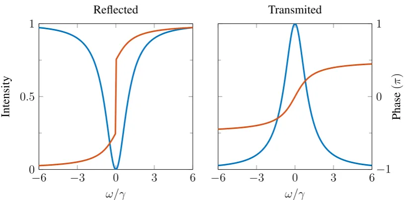
[image:46.595.77.485.90.291.2]

−6 −3 0 3 6−1 0 1 ω/γ Phase ( π ) Transmited

Figure 2.5: The intensity normalized to the power of aic,in(blue) and phase (red) of the

reflected, aic,out, and transmitted, aoc,out, fields using the classical analysis of the cavity

fields. The cavity parameters used here are from the cavity discussed in Sec. 3.2.2. The fields aoc,in and al taken to be vacuum modes. The discontinuity in the phase of the

reflected field is caused by the reflected field disappearing when the cavity is on resonance.

The output fieldsaic,outandaoc,outin the Fourier domain can be found by using the

bound-ary conditions,

ˆ

am,out = √

2γmˆa+ ˆam,in, (2.26)

to give,

ˆ

am,out =

(γ+iω−2γm)ˆam,in−2√γmγnˆan,in−2√γmγlˆal

γ+iω . (2.27)

Herem, n= {ic,oc}. The classical analysis of a cavity can be made using the linearisa-tion of operators in Eq. (2.27) and ignoring the fluctuating terms. Settingαoc,in=αl = 0

gives the transfer functions from the input fieldaic,into the reflected,aic,out, and

transmit-tedaoc,outfields,

αic,out

αic,in

= 2γic−iω−γ

iω+γ (2.28)

αoc,out

αic,in

= 2

√_γ

icγoc

iω+γ (2.29)

Whenω ≈0the cavity will have maximum transmission of the input fields,aic,inand

aoc,in, through the cavity. On the other hand whenω≫ γthe cavity will reflect all of the

input fields e.g. ˆam,out = ˆam,in. The 3 dB point of a cavity is given whereω = γ. This

(47)

Second order optical non-linearity 35

2Ω Ω

Ω

2Ω Ω

Ω

(a) (b)

Figure 2.6: Second order non-linear process. Down conversion, (a), takes a single photon of frequency2Ωand produces two photons of frequencyΩ. Up conversion, (b), takes two photons of frequencyΩand converts them to a signal photon at frequency2Ω.

noise limit whenω ≫γand the other inputs are vacuum modes.

2.3 Second order optical non-linearity

When an optical field is passed through a dielectric medium an atomic polarisation, P, is induced on the dipole moments of the medium. With light far detuned from the reso-nance of the medium the electromagnetic field create a macro-scopic atomic polarisation oscillating at the frequency of the field. These oscillations can be re-emitted back into the optical field. In a non-linear medium these oscillations can occur at harmonic frequencies of the original field. The polarisation of the resulting optical field can be written as the series [21],

P =ϵ0 (

χE+χ(2)E2+χ(3)E3+. . .), (2.30) where χ is the linear susceptibility and χ(i) _{is the} _{ith non-linear susceptibility of the}

medium. The second order non-linearity, of interest in this thesis, are used to either generate a second harmonic or squeeze a quadrature of the fundamental field. This thesis will limit the description of optical non-linearity to degenerate parametric down conver-sion. This is a simple case of non linearity where a single photon in a pump field,b, of frequency2Ωsplits into two photons of the fundamental field,a, of frequencyΩin some non-linear material. The non-linearity of the material is parameterised by the second-order non-linear susceptibility,χ(2)_.

Phase matching condition

As with any system both energy and momentum must be conserved. In a degenerate sec-ond order non linear process the energy conservation is satisfied by Ω2 = Ω1+ Ω′1 and

momentum is satisfied by the wave vectors k2 = k1 +k′1. Here ’ is used to represent

Protocols and Resources for New Generation Continuous Variable Quantum Key Distribution