Alternating direction implicit methods for partial differential equations

ALTERNATING DIRECTION IMPLICIT METHODS FOR

PARTIAL DIFFERENTIAL EQUATIONS

Graeme Fairweather

A Thesis Submitted for the Degree of PhD

at the

University of St Andrews

1966

Full metadata for this item is available in

St Andrews Research Repository

at:

http://research-repository.st-andrews.ac.uk/

Please use this identifier to cite or link to this item:

http://hdl.handle.net/10023/13784

W T

ALTE&NATIBG DIRËCTIO» IMPLICIT METHODS

FOR

PARTIAL DIPFEREHTIAL EqUATlOHS.

A th#ais presented by Graeme Falrweather, H#So.,

to

the University of St# Andrews» in application for

the degree of Doctor of Philosophy.

ProQuest Number: 10166974

All rights reserved INFORMATION TO ALL USERS

The qua lity of this reproduction is d e p e n d e n t upon the qua lity of the copy subm itted. In the unlikely e v e n t that the author did not send a c o m p le te m anuscript and there are missing pages, these will be noted. Also, if m aterial had to be rem oved,

a n o te will in d ica te the deletion.

uest

ProQuest 10166974

Published by ProQuest LLO (2017). C o pyright of the Dissertation is held by the Author.

All rights reserved.

This work is protected against unauthorized copying under Title 17, United States C o d e M icroform Edition © ProQuest LLO.

ProQuest LLO.

789 East Eisenhower Parkway P.Q. Box 1346

' . ' Vf , " / ..V. yW:

(i)

I

(u )

P W A G B .

In October i960» I matrloulated at the University of ^t$ Andreiifc and read for a degree in Applied glathematloe In Bt* Balvator^e College# In June 1963» I graduated with Flret Olaee Boncure In Applied

Mathematlee# In July 1963» I w e admitted» under ordinance 16, ae full-^tlme Reeearoh Student In the Department of Mathematloe of 8t# Salvator's Oollege under the oupervleion of Dr A# R# Mitchell#

A o m o u L m m m i m T #

I certify t W t Graeme Falrweather hae epoat nine terme in fall«#tlme reeeareh work under my dirootlon# and la thus qualified to 8%A>mlt the aooompanying theele In applioation for

J 0 & 2 S L 1 * iMaomoTioia

1* Introduotory remarke# 2

2* Finite dlfforenoe metho&e for the solution of

partial differential equationo* 5

3# Stability and convergenoe of initial value problème* 10

4, Oonvergenoo of iterative prooeduree# 17

q m p œ II. igeaovBD Ai T m m A fi w DiRBOTio:^ iwiiciïP

FOR PAIÏABOLIO AMD m,LIPTIO mUATIOIifS Ih TWO 8PAGB

VARIABLE.

1* Introduotion. 20

8* The ADI methode of Peaooman# Douglas and Raohford# 21

3* Generaliaed P*R$ and D*a* formulae, 24

4# The optimu;a formula, 26

5# Alternative derivation of optimum formula, 28

6, stability of P,R*» D#%, and optimum formulae# 30 7, @lodifiod ADI method for non**%ero boundary oonditiona, 33 8# GeneraliBod iterative procedure for Laplace*#

equation, 36

9, Optimum convergence factor, 39

10, Metbode of oelooting eequencee of iteration

parametere, 49

(v)

'5>-12* Footaoto*

13# Ilumcrioal G3#@rim@nt8 14# Concluding remarko# Appendix

5# 6 *

8#

[I# impRovm) ADI mrnoDs T i m m SPAOË VAHIABL@8, Introduction.

The Douglao';~Raohford and Douglas methoda. Generalised D.R# and Douglas formulae# The optimum formula#

stability of the optimum formula.

Generalised iterative procedure for LaplBoo'o equation.

Optimum oonvergenoe f&otor#

$equ8&ooG of iteration parameters.

CHAPTm IV# A API MBfROD FOR THB: BIHARMOmiC

m w a * 1^ Introduction*

2. The Conto-Damee (0.#,) method. The generalised O.P. formulae#

Oonvergenoe of the iterative procedure. Optimum convergence factor.

3# 4 . 5# 5 3 5 5 64 Solution of trldiagonal syotome of equations. 6)

68

6* Concluding remarks# 100

Appendix, Solution of quidiagonal systems of equations# 101 continued overleaf#

-(y\)

Q i u n m V. h HIGH AOOOMOÎ A,PI f W H OD FOR TOi!i BâVË ËttWAÆIOa. «MÉ«Iww##w#W#Mii'#ip.i• Will ... -T^-—r-'-' -‘ iirm^ irTr- mriinr^ ir'-ir^'irrirr-mr/nnmTiiTi'n'iimi'iii

1# I#trod#ot&6&* 104

2# The methods of Konovalov and two, lOg

3# OonoralisGd ADI method and an ADI method of

Inoreaeod aoour&oy, 10?

4* Stability* lOg

9* The throo#^epaoo variable oaee* 111

6* Numerical expérimenta. 114

GOKCLumiaG ii8

%

I#l, introduotory Hesmrka,

Partial differential equations ooour in moot brmnohee of applied m&thematlos, phyeios and engineering, Wany of the linear problems which arise involve the solution of an equation obtained by suitably specialising the form

where \ and^ are certain physical constants. Her© the operator ie the haplaoian operator in the space of one, two or three dimensions* For example,

&

in three dimensional rectangular coordinates, where the unknown function u is a function of the space coordinates %, y, a and the time coordinate t.

In particular, Laplace's equation*

(1.1) V ^ U . = o ,

is satisfied by such physical functions as the velocity potential of an ideal incompressible fluid, the gravitational potential in free space, the electrostatic potential in the steady flow of electric currents in solid conductors and the steady-*state temperature distribution in solids,

The wave equation*

(1.Ï) X ) V = | k

and by the velocity potontial In the theory of sound (acouotloo) for a perfect gaa#

The diffusion equation#

(1.3) V V =

io catisfiod, for oxomplo, by the température at a point of a homogonocuc body and by the oonoontratioA of a aubntanoe in the theory of diffusion, whore p io & suitably proooribed oonotont#

Differential equations of higher order involving the operator V^ero also frequently encountered. In particular, the biharmonio equation in two dimencicnc,

U.4) v V . o .

is involt^ed in many problems in the theory of elaotioity# The

wmm

equation also arioeo in the dinoueeion of the alow motion of a viecouo fluid#

8olutiono of tbeee equations for regions of wbitrary shape arc, of course, not known, but oven for thooo problème for whioh analytic Bolutiono in eerioe form arc available, the eorioo often do not lend

themcolvoc rogdily to numerical caloulationo# Direct numorioal oolutiona of thêoo oquationo ere therefore of oonciderablc importance#

There arc many numerical méthode for solving partial differential equation#* Of those, only one otando out m being unlvoreally

applicable to both linear and non^^linear problem#— the method of finite differenooc* It i# the major purpoco of thi# thocie to attempt to

-.laetboda, for aoivlng sovaral types of llnocir partial differential equations. In Ohaptare II and XXI§ high aceuraoy ADI methods for equation (1#3) in two and three apace variables are derived and, as a result, families of iterative techniques for solving

(1*1) are obtained. ADI methods for the numerical solution of (1*4), and (1.2) in two and three space variables, are discussed in Chapters IV and V respectively* All numerical calculations were carried out on the IBS 1620 computer of the University of St* Andrews*

1*2* Finite Differ&mo# Method# for the llûlutioa. of Partial Differential Kgytcitlone*

%very partial differential equation is either of elliptic, parabolic

or hyporbolio typo, for o%a;%plo, (1*1) and (1*4) are olliptio partial differential équations while (1*2) iG hyperbolic nnd (1*3) ic parabolic,

(see Sneddon [39])* Problems of parabolic or hyperbolic type lead to

initial value nroblemo einoo the conditions at time t # 0 ore specified

m

m

dependent variable in then calculated for t > 0# On the other head,

elliptic eqmtione load to boundary value problems» In thin came, we

must find a function which satisfice the differential equation and aloe

conditions on the boundary of a oloeocl region*

The method of solution by finite differenoee depends on the type of the partial differential equation but the mein approach ic to cover the domain of the independent variables by & rectangular network of p l m m $ not ncaceoarily equally spaced, but parallel to tho principal

planes* The finite net of pointe^ of interjection of the planes constitute the meqh .pqintm* or nodem# and we meek to determine approximate values of the desired solution at these points* The values at the mesh pointe

are required to eaticfy difference equationo obtained cither by replacing partial derivatives by partial difference operators or by certain other more aophiaticated techniques*

The method in beet described by means of an elementary example* Consider the parabolic equation

subject to appropriate initial and boundary conditions# This equation may be written in operator form

(1.5) ( & + Dp - »^)u - 0.

In this example and throughout the remainder of the thesis, the domain of the variables %, y will be square or rectangular and will be covered by a square mesh where « Ay # h# The natural and simplest finite difference representations of and D are

where 6^ and 6 , the central difference operators in the % and y direction# respectively, are euoh that

&%«(%,3f,t) . «(x+'|h,y,t) - u(x-|h,y,t) and

&y«(*»y#1î) « u(x,y+-|D,t) - u(x,y--^h,t). There are two equolly natural reproéentationc of

where k is the meeh else in the t-direotion and and are the forward and backward difference time operators respectively where

A|.u(x,y,t) o u(x,y,t4-k) - u(%,y,t) and

V^u(x,y,t) - u(x,y,t) - u(»:,y,t-k).

If applied to (1,5) with . ^ = w(3Cj^,y^,t^) where » ih, y^ « jh and t^ m nk, these forward and backward time operators lead to somewhat different difference equations which can be written an

P ( " i , 3 + l , n *1+1, j,n •*• + *1-1, j,«) + “

'*■ “ i , 4 , » + a * ®

roKipootlvely^ whoro r 6% k/b^ lo the moek ratio# The oooffiolonto in t W # o approximations can be ropro8ento& eohematioally In tho follo^lne way*

Those oohomao show the relative loo%tlono of the pointa to whloh the

ooeffioiente m m applied# f h e first mothod# ( 1 . 6 ) * the forward differenoe method# io an example of

m

mmnà

t^e. ha,ckward, dlfferenoe. ,me^hpd# le mm example of km Implicit method, à diffèrenoe method being termed explicit or Implloit aooording to whether eaoh of the différence eqwatlono at t

m

mmmi'l

etop of the calonlatlon io much oaeier for an explloit method than for an Implicit one ** on oxpllolt method rotinlree at each step the solution of a number of equations with only a single unknown in each of them,

while an implicit method demande the solution of a aystem of oimultaneouo linear equutiono* Unfortunately, moot of the explicit metbodo are only conditionally qtoble# and tbio impoeeo an upper limit on the allowable mesh r&tiOB, The concept of gt&bility ie diocueoed in tho next section#

BtèB-by-step in time using a so-called "marching" prooeas. for elliptic problems* on the other hand, the solution cannot be found at any specific point without being found at all points* fhio fact is borne out by

the following example*

Oonsider Laplace'e equation in two dimenciono

% 'xA.

1 5 ^

with appropriate boundary eonditionç* In operator notation thie equation may be written m

+ flpU - 0.

The most common finite difference replacement ie obtained by putting # # _{X 3C} and _{*r */} yielding the formula

at the node % * ih, y « jh# The application of this formula to each node in turn together with the boundary conditions yields a set of

linear equations for the unknown nodal values u. .. Thus, the solution_{1 , 3} of an elliptic equation by finite difference methods reduces to the solution of a system of simultaneous linear equations* however, since there is one equation for each mash point and since there may be several hundred mesh points, great care must be taken in the choice of method for solving these equations, in case the computing time, oven for a very fast digital computer, becomes excessive* Iterative methods arc indicated because of the large number of aero elements in the matrix of the coefficients, and are nearly always used# With such methods, we take an initial approximation to the solution and successively

that is, until the difference between suooeeeive estimates of the exact solution is less than a prescribed amount* The problem of stability does not arise in the solution of a boundary value problem involving

a linear elliptic partial differential equation* However, the oonvergeiio< factor of the iterative method is of critical importance, and io

disousçéd more fully in 1*4*

One iterative method for the solution of the equations arising from the application of (1.8) to each node is the method of Altman or Von llieea (Martin and Too [28]) which may be written in the form

(1.9) *1+1, j * " ®»

I tt ^

where u} % denotes the n th estimate of u. . - the exact solution of the

i f j * t 3

difference equation’at the node (ih,jh) - and d is an iteration parameter which is chosen in order to accelerate the convergence of the method* It is easily seen that there is a great similarity between (1*6) and

(1*9)* in fact, if, in (1,6), r io replaced by & and each time step is regarded as m iteration, wo obtain (1.9)* This connection between finite difference methods for the solution of parabolic equations and iterative methods for the solution of systems of equations arising from elliptic difference equations is employed in ohaptors II and III*

Just as (1*6) had its limitations for solving the parabolic equation GO (1*9) ia not one of the better iterative methods for the solution

to

1*3, stability ..and Oonvergance of Initial Value Problems#

When discussing the numerical solution of partial differential equations of parabolic and hyperbolic types by means of difference methodsI m must consider three distinct solutions, namely 1) the theoretical solution of the differential equation, 8) the theoretical solution of the difference equation# and 3) the numerical solution of the difference aquation# The difference between 1 ) and 2) is due to trunoation error% the error introduced by dieorotising the problem# This error may be defined as followo: let the differential equation be rewritten as the differential operator equation

Du » 0

and the difference method be written as ^\x 0

then, for any sufficiently smooth ftmotion v, we define the trunoation error as the difference

l)v ## z*v#

As an example, consider the difference equation (1*6) ae an approximation to the differential equation (1*3) with ^ « 1, and two space variables, and let u(%,y,t) be any function with continuous

partial derivatives of sufficiently high order# By eaipanding u, . .,n u. jL n ^ 9 etc#, in terms of u, . ^ and its derivatives, where

u. . ^ * u(ih, jh#nk), we find that the difference between the finite difference expression and the corresponding differential expression is

The right hand eide of this • equation is the principal part of the

trwoation error of the difference scheme (1,6) and is a measure of the acouraoy of the scheme& The fact that the coefficients of At and of on the right hand side of this equation are bounded - from the assumed continuity of the partial derivatives occurring io'oxpreosed

followss (1.10λ)

+ “l,3,n+l^/^'‘ •*■ % " & “ % A , 3 , n ”

as At, II 0#

This equation is to be interpreted as meaning that there exist two

positive constants A end B such that the absolute value of the left hand side of (1,10b) is less than or equal to A At for all sufficiently small At and h# Such a difference scheme is said to be second order correct in space and first order correct in time.

The estimate (1,10b) of the trunoation error holds in particular if u is the exact solution of the differential equation and, in.this case, the second term on the loft hand side of (1,10b) vanishes. Furthermore, using

- A l + + i l k .

from the differential equation, and At « rh^, the right hand oido of (1,10a) becomes

- U * * ^

and io said to be of order ti* # [see I m m n [2?], section Vl],

solution of the difference equation tends to that of the differential equation m the mesh is made finer and finer, that is, the problem of convergence. It was found some years ago by Courant, Friedrichs and Levy [9] that certain conditions must hold between the inorements of the independent variables for convergence to occur.

Hound-off error causes the difference between 2) and 3) end can give rise to the phenomenon of instability, Roughly speaking, if a difference equation is unstable and if an error such as a rounding

error is made at any stage of the computation, this error will increase exponentially as the number of time steps increases, end, eventually, the m^lculated values of the solution of the difference equation will bear no resemblance to the theoretical solution. Von Bewa&nn [31]

proposed a criterion for investigating this problem for linear equations with constant coefficients, and his criterion showed that stability

occurred when precisely the same ratios as called for by Courant, Friedrichs and bewy held, Douglas [173 has since shown that, for

"wide elasses" of difference analogues of linear parabolic and hyperbolic differential equations, stability in the sense of Von leumann implies convergence.

Various aspects of stability have been considered by several authors# Lax and Elohtmyer [24] give a definition of stability in terms of

13

analyses by mesne of the direct estimation of the eigenvalues of the matrices induced by difference operator».

linoe the difference equations with which we are concerned in this thesie are linear with constant coefficients, Von Neumann*e method le used to examina stability. Using operator techniques similar to those of Todd [43] and Lowan [8?], we now give a definition of stability in the sense of Von leumann, We shall consider for the moment the numerical solution of a linear partial differential equation in the region

0.4rx,ykl, t ^ O for which the solution io specified on the boundaries and sufficient initial conditions (that is, value of the function for, the parabolic case, the function and its t-derivative for the hyperbolic case, or more if of higher order) arc given to ensure the existence of the solution of the problem, Let (Bfl)h » 1, » ih, y^ # jh, t^ ^

and denote f(x^,yj,t^) by f^ Let be the solution of the

difference analogue of the differential equation, further, let 0

represent the column vector any

partial difference equation may be written in the following matrix form*

(l,U) • AqU^ + + ... -S- «>0,*

where io non-singular and b,^containa the boundary conditions, (A^ is the unit matrix for explicit equations. ) For (1,11) to be

other source into the vector U_and oall it U^^'# Then, step ahead using (1*11) and call the perturbed solution U^. The resulting equations become

•^xkffl+2 “ ' ^ A + 1 ■*■ ^-l-'m + + ^‘-qüni.g+1 + &m+l

^ 1 % + 1 “ ■'• *

Let

(1-13) â «

Then

(1*14) ■*■ ^-l^n-1 + * «3- m-Hi

\inj»-^m,+l » ••• > lm+% determinea by (1.18).

We note that (1*14) is nothing more than the homogeneous equation

corresponding to (1*11)• Ae A. io time-independent, m may be taken to be zero#

Von Beumann*8 technique is to apply the method of separation of variables to (1.14), (oee 0*Brien ot al [31])* For this method to bo applicable, it in necessary that the matrices A., i * 1, 0, **, , -q, poseeoo a common set of eigenfunctions (p , p,a * 1, **# , N* This_{J Pfc?} ie equivalent to requiring that the matrices A^ commute^ We allow the identity matrix to have any complete orthonormal sot as eigenfunctions* Consequently, we must restrict ourselves to such difference equations* Let

15“

£ » •

Binoe the error equation is linear, we need only consider one term in this eapension, end, in faot, we may take

*

( 1 . 1 6 ) ^ Then

(1.17) , ‘Apg^\+x “ r • • • 9"

It is well-known (Milne Thomson [2g]) that the general solution of (1*1?) is

( 1 . 1 8 ) % - g ° 3 f “ s*,1 ■

where the . ere the distinct roots of

( 1 . 1 9 ) p ' - --- - 0 . If a root p is repeated t times, a term

^ d^n •# # * * 4*

repleoea the corresponding t terms above# Mote that a grows if max > I* decreases if max

L

max “ I Bnd no multiple root has modulus one, and grows slowly if a multiple root has modulus one* Thus, only in the first ease does the error grow significantly in a reasonable number of time steps#

llonce, the following definition of stability will be adopted# Equation ( 1 # 1 1 ) io stable if and only if

(1#30) max j| ^ I# 4 ^ 1 # • * # * # q^t'lf p,s ^ 1, * * « ,M* In this thesis, we shall consider only the caoo where the roots are

distinct#

(t»

these formulae, the oigenfunotlons (not normalised) may be taken to be

(1*21) ^ps ** [êln sin ^ o y «5 X, » * # , H,

(see Rutherford [38])# It may readily be m o n that the eigenvalues of the A. matrix are, reepeotlvaly,

^ps * ^

(

1

,

82

)

/\^ « 1/r f 4[ain^%p/0(m4l) > siï?rîs/2(I-fl)]*_P0 Moreover, the stability ratios are, reapeotively,

(l#23a) p # 1 - 4r[0in^np/2(M4*l) t eiii^it0/2(I+l)]

(1.23b) p ** l/[l 4^ 4r(ein^wp/2(Mf 1 ) *¥ eW%e/2(M+l)]#

Thus, from (1.20), the forward difference formula is stable if 0 ^ r - y while the backward difference formula ia unoonditionally etable. that is, stability is guaranteed for all positive valuee of r#

A simpler method of examining stability of difference formulae based on the above analysis io the following# Instead of considering the error vector wo shall ooeider one of its components,

^

and, from (1*16), we put

(1#24) j,n ** \ûinîtpx^sin?«sy^i p,s » ! , # # # , M,

where, in general, the difference equation applied to the node (ih,jh,nat) does not involve boundary points* The error component £ ^ ^ ^ then

satisfies the same equation m For example, considering once again (1*6), the error equation is found by replacing u by 5 . Using

(l#24), we find that

JS±à « 1 - 4r[ ein^ %p/2 (#f 1 ) f sin^'ji©/2(I*fl)] which ie seen to bo (l#23a)* He then require p

f\

IV

1*4* Convergence of Iterative Procedures.

The method aiGOuaoea la 1.3 far examinin# the stability of &

finite difference replacement of a partial differential equation may be uecd to examine the convergence of on iterative procedure for the

solution of an elliptic difference equation. As an illustration, consider the iterative formula (l.g) for the solution of (1*8), It may bo written in the matï*ix form

(1.85) + b

where the vector » » . • . . the vector ^ is

determined, by the given boundary data. Me define the error vector,

E m . U

as the discrepancy between the approximate solution and the exact solution Ü of the system of equations

(1 ^ A ) U . b,

The object of the iterative procedure is thus to reduce the components of the error vector to mere# For (1,25), the error equation is

(1.26) ^ + 1 “

As in'1.3, we consider

where g) , p,o, « 1, . * , , #, are the eigenfunctions of A# As before, iPpe " Cein apa^sin %Gy,] p,s * 1, . , , B. Thus, for the procedure to converge, we require that

(1.27) max A: 1 P,s 3.1 . . . , H|

IS

must be of wodwluo lees than or equal to one# For thle example, "Xpg * ^ ~ 4olC8in*%p/k(M*l) +

and GO, for convergence, we require

(1*28) cl t: *

In order to obtain the beet, that is , the moot rapidly convergent, iterative formula, wo minimise max |A | with respect to ço that the components of the error vector are reduced to aero no quickly m possible# A simple calculation shows that the required value of d is

= X •

The optimum convergence factor is then given by

In chapters II and III, the convergence of iterative schemes is investigated by considering only one component of the error vector , as in I# 3,

GHAPTBR II.

5.0

11*1* Introduction»

Alternating direction implicit (ADI) methods are usually n-atep procedures for the numerical solution of partial differential equations in n space variables* The difference equations used at each step are implicitt but the systems of equations arising are of a particularly simple form and may be solved by a direct non-iterative method* The first ADI method was introduoed by Peaoeman and Haohford [34] in 1955 for the numerical solution of the diffusion equation in two space

variables, and the term "alternating direction method" arises from the fact that in the first stop of this method we solve along horizontal mesh lines and in the second step wo solve along vertical mesh lines, or vice versa* This will become apparent later in this chapter*

11,8, The ADI Metbodo of Feaceman, Oouglac and Hachford*

Oonsidor the diffuBlon equation in two space variables

(2 .1 ) ^ ^ ,

where the temperature u is a function of the epac© coordinates x,y and the time t, The initial and boundary conditions are u(K,y,0) « f(%*y) over the unit square 0 «11 and u(x,y,t) » 0 for t > 0 at points on the boundary of the unit square, respectively. The assignment u * 0 on the boundary involves no essential loss of generality from an

arbitrary, sufficiently smooth specification of boundary values. Other boundary conditions are considered in XX,7 •

The ADI method of Peaceman and a&chford [34], (see also Douglas [14]), which is referred to ae the P,R. method, may be written in the form

(2,2a) (-&rt^ + l)Ujj^|, - (àr6y + l)u^

(2.21,) C-àrb^ + » (ârü;. +

where 6 are the usual central difference operato&a in the % and y directions respectively, u , u^^i and _{iii niHr K mHrX} are the values of u at the nodes (iz^z, ja.y,#/\t), (i A x , j/hy,(m4*|) At) end (i Ax, j Ay,(m+1) At)

respectively, (i,j « 1, 8, , . , 1-1$ m * 1, 2, » . .), Ay and A t are the mesh lengths in the %, y and t directions respectively and r m At/h^, where A x * A y «« h, is the mesh ratio. Elimination of u ;j. from (2,2) leads to

-point operator

0

An alternative form of the P.R* method, given by Douglas [11], ie

(8.'4r) (“i|r5^ + = ( # 6 ^ + rfcy + l)«^

(8.4h) (-^Cy + " '^S+l “

where denotes an approximation to Elimination of again yields (2*3)# The value of this formulation will become evident when alternating direction methods for three space variables are considered in Chapter III# However, at preeent, we oonGider the p#a, method in the more convenient form (2#2),

e second ADI method, the I)#IU method# vme formulated by Douglas

and R&ohford [12] and is given by

(2* 5a) - (rt^ + l)«j

(g.5b) (1*6^ + l ) V l

-y&+l &#&1% denoting an approximation to WL+i* Formulae (2*5) lo&d to

(

2

*

6

)

after elimination of _m+i , where (-rtr _y 1 )(-ro ^ l) and (1 + r^o b )_{À ^ ^ X y'}

are, once more, nine-point operators.

A generalised formula which involves nine-point operators on each of two neighbouring levels of time is

(2.7) fl + A(i)^ 4- ô p 4. » Cl + C(b^ + b p

9.3

both be G%pr@8Ge& in the form of (2,7), Xn fact, the oooffioiente are

A B 0 * #r, D =

for the P,B* method, ami

A " —r , B » r*^| 0 * 0, I) *» r^, for the B,B* method,

Alao, expanding (2*3) and (2.6) &B Taylor eeriea in terme of um and its derivatives and replaoing derivatives with roopoot to t using

the relations « V^u, etc,, from (2*1), where

+■ it is easily shown that the principal parts of the

truncation errors are

t'"'# *

;

for the F *11, method and

for the D,K. method.

In the first section of this chapter, values of A, B, 0 and I) are

found which eliminate the terms of order h^ in formula (2,?) and the

II#3• OoneraXized P,R# and i)»E# Formulae# (Mitchell and Fairv/eatlior (193)

In its present form, formula (2,?) is of little use as a means of solving (2,1) oinco, if Mh « 1, it requires at each timo step the

solution of (N-1)^ linear equations in (B-l)^ unknowns* However, if

(2*7) can bo written as a pair of F *11* or D*B* type formulae, that is,

a pair of formulae which utilises the same points as the )?*E* or i)*lU formulae, the numerical calculation involves the solution of (K-l) equations in (B-1) unknowns first along lines in the x direction and next along lines in the y direction* At every stage of this scheme, the matrices arising are tridiagonal, or Jacobi, matrices* Bueh systems of equations can be solved directly by the algorithra outlined in Appendix II*A at the end of this chapter*

Considering first the points used by the P.H* formulae, we may write (2*7) as

(J?.8a) (Ab^ . (01Ç + l)u^

(2.6b) (Ao; + -

(Ob-provided B *• A^ and I) « 0^* 33ext using the same points as the D.M.

formulae, (2*7) can bo written as

(2.9b) (Ab^ l)u*+i - C(0 - |)6y + (1 - %)]«,

(2.9b) (Ab- 4. . (| b; + f)«^ 4.

Formulae (2*6) and (2,9) are the gonorallzod P.R* and D#E* type formulae roopeotlvely and formula (2.?) oannot in general bo repreGented by (2*8) or (2*9)* If, however, B » A ^ , (2*7) can be written as the

:#4* T h e O p t i m u m F o r m u l a #

Me now expand the terme (5^ 4 etc#, in (2.?) as

Taylor series in terme of u^ and ito derivatives, replacing time

dorivativeo by » V^u, * V*^u, etc#, from (2#1) where

^ ■'■ • The expansions up to and including terras involving

are

“rft+l - " + -*• ’» ^ 2 + + ir^Ag

(^x •*■ S^**m+X “ + È^Ag + SrA^ + (fïï*'^ +75?

*-+ ( K *-+fkr)A5 /LX y“»M.l - •*■ (r + i)Aj.

+ ô p « , - + îïA^ +

^x^y\ " *3 + à:*5 where

■*■ * ^'2 " ôÿ) • ^3 “

& " ^ %)'

“

+ %) •

If these expressions are substituted into formula (2,7), values of A,

B, 0 and D can bo found which will ©Xiniinato A^, and oithor

i\^ or Ag. However, a formula of type (2,7) lo orily of use ao a moans of solving (2.1) if it can at least be written in the form (2,9)# Thio will bo pOBoiblo only if B « A^# Hence, the coefficients in the

optimum formula are ohoson eo that they eliminate A^, Ap and and

tL^f

à « -è(r - B w -ç(r - ,

0 m # ( r + % ] , B « -^(r 4' #

The formula of typo (2*7) with minimum truncation error which can he written in the form (2*9) ie thus

(2*10) [1 - M r . ^)(h^ + + l(r

-- [1 + i(r + + b p + ^(r + feHpUj .

The principal part of the truncation error is in fact

” t lÿ) »

wîJlob is stt ordea? better than the original B.B» or P*H. foasaula.

It also follows that if r is approximately equal to 1 / 8 , the

truncation error may ©yen he of order if, When r (2*10) degenerates

into the well-known explicit formula

- a - * ‘p

-and GO the method of alternating directions ie inapplicable*

Formula (2*10) can now he written ao the D*i# type formulae

(2.lia) C - ' K r + 1]%+1 " Ei(r + i^)by + 1 1 %

(a.llb) C-è(r - i)by + 1]%^1 - - Hf(x + ^)6y + I l% +

and, mince the optimum coefficients satisfy D # 0^ a© well an B * A*"#

(2*10) can also he written as the P*R, formulae

(g.iaa) C-I(r -t)&% + l1%+iV “ + 1 ] %

1 1 * 5 * A l t e r n a t i v e D e r i v a t i o n o f O p t i m u m F o r m u l a *

Originally, it

mm

that the P*E* and D*R* methods ware intimately assobi&ted with the

Crank-Bloolson and backward difference analogueo of the diffusion equation

respectively* The eonnootions between the P*E* and D,a, methods and

these simpler formulae become apparent when equations (8*3) and (2*6) are rewritten in the forms

(2*13) % + i " % + "m) "

and

V x “

respectively* From formula (8*13), we see that the P.#* method is a perturbation of the Orank-Mioolaon formula and is thus second-order correct in both space and time, and, from (2*14), the l)*E* method is clearly a perturbation of the backward difference formula and is thus second-order correct in space but only first-order correct in time*

(Bee Hiohtmysr [3?] Table I page 93)#

Consider the formula

(2*15) \ + X " "m + + 1 ) % + M r

14

formula as a pair of P#B* or B.B* type formulae* Suppose this perturbation is of the form

(2ml6) ^ ^pCè(r +&)*% + *(r - %

+ % ( p \ + i - °

where p and q are parameters which are functions of r# Writing (2#l6) in the form (8*7), we find that

A « -&(r B » p , G m -§(r + D « q.

Hence, if p * %(r - if* and q * %;(r + formula (2*16) can be

3D

m à

Th@ stability of formula© of type

(

#?)

procedure outlined in 1*3 . We aooumo that there ooioto an error

^iij.m Güoh moeh point (i&%,jj&y,mz^t), (i,j

«

,

, , * ,

m

1

£sy

expanded in the form

iip%ein (p,Q = 1, «, . . , K-1),

whara « i/^a, y, * jZ^y, and substituted into equation (2#?) with u

d by f and «* A y « h * 1/m, it follows that

(p „ I ^ ÀQiBinh^vMîî •¥ sinStq/2M) + l6Doin^*io/?E B i n ^ m M î

a _m (-4AsiW'*'ap/ai f 1 ) (^4Aein^)kq/2M + 1

where use has been made of

o^oin ftpx^ iss -4ein%p/2M sin apx^ , (p * 1, 2, . . , #*1)

and B * the condition neoeeeary for (2.7) to be written in l)*E*

for*m. Thus I for the D*E* method

f T H ^ T i ^ r T B ^

where 8^ ■« 4ein^)&p/2E and * 4Bi.n'nq/2M^ This ratio clearly has an

absolute value less than or equal to unity for all p,q in the range

1Ax>,q,AI-1, and r > 0 and hence the D.E# method is unconditionally

stable* It is Interesting to note that if equation (2*5&) were used for every time step, then

1 - rS*^

For some values of and r, this ratio has an abeolute value

considerably greater than unity# Henoe, such a procedure is highly unstable* A similar situation arises when formula (2*2&) is used for every time step. Formula (2,18a) cannot be used at every time otep as it is inconsistent.

If 1> « O’^ in addition to B » equation (2,7) can then be written

in the F,E, form and the numerator of (8,17) factories# to yield

,, f m l (-03^ + + 1)

' ' ' a„ * (-AS^ +"l'y(“AS'^' V l) ‘

» p g

Hhen A ■ — 0 • ir, this ratio again has an absolut, value less than

unity for 1 ^ E-1 and r> 0, Hence, the P.R* method is unconditionally

stable*

For the optimwa formula (2*10), equation (2*18) becomes

» X *^a eay,

a

In order to prove that -l^=-^^il, it ie sufficient to show that m

M r +-L)a^u»l v(u) = î i F T n s j r ï

«

an absolute value less than unity, since ^ « V(p) and jjl V (q).

has

For this to be true, we require

ra]" 0

3 1

3%

XI•7• Modified ADI Method for Mon-%ero Boundary Conditions*

When the boundary condition© oro non-sero, the ADI method given

by (8*18) requires modification. If we conoidor the totality of the difference équations (2*10), we obtain a oyotem of (M-l)^ linear

equations in the (M-1)^ unknowns u(ih, jh,(m+l)At), (i,j « 1, 2, * , ,î!-l) where m is fixed (ra » 1, 2, • • • ), which may be written in the matrix foritï

(2.10)' [1 + i(x %)(» + V) + L(^»

-= fl •» K'(x + a){li + V) ■!• ■'■■ %)'' o ,

where I! and V are the matrices of order (l-l)^ given by

11

n

21 -I -T 21 -J *

, and

«f« «.(I «#* 44*

* *

, *

-I 01

respectively, where II is the matrix of order (M-1) given by

2 -1

-1 2 -1

-1 2^

and I is the unit matrix of order (E-1), and

where k* and » (n # are constant veotora whose tth components are obtained .from the boundary values occurring in (b^ f b^)u(lh,jh,n At)

end u(ih, jh,nAt) respectively; where H ** (B-l)(j-l) -f* 1? The

modified ADI method takes the form

(0,18a)' [I + &(r - = 0- - &(r + 4 a

(e,12t)' [I + #(r - t + %

where

1 ? ^ V . S". - M M ï'„i s:,*i

and

t « . ,.(??,':.Ukt,D. 1,1 . ( r . | f „(r+%j. ^ istit. k« , + ii±s'^

— 4r “ ill"’ '"ér" — a*’ 4r — m+1 ^ 8r ^m<-l *

Thio modification means that, if, in (2,12&) a boundary value (loft

{ . la involved on the s hand side, the term involving

|^%(ih,eà) [right

this boundary value ia replaced on the right hand side by

l-eft right

and if, in (2•12b), a boundary value < ‘ is involved on the

hand side then the term involving this boundary value is replaced on the right hand side by

35*

f

1 4r » “1 " " 2 4? ' "2 4?

o.ncl

“ a '!' (r + g- )«^], _V^* i>~ “ f l - (r -_{«iL ^4,}

IJhen boimdary values occur on both eldoo of (2.12a) or (2.12b) they are replaced ao prescribed by {^) or (**) and tix;; coefficient of the bomidary value coimrion to those replacements is halved,

The A.DI method (2.11) way bo modified in a similar manner to take

the form

(2.11a)' [I 4 &(r - t)H]u%_ , ^ _{’134*1 (^* '" i)} [% ^ #(r t)Vlu 4 o_{^ — m}

(2a i h ) ‘ [1 4. i(r - - - If-id) c:i - M r 4.

The ADI methods formulated in Chapters XXI and V of this thooic are

36

11*8, Generalized Iterative Procedure for Laplace's Equation#

In this section, and later in Chapter III, we make use of the heuristic analogy between iterative methods for solving elliptic partial differential equations and numerical method© for solving

parabolic partial differential equationo, (see Varga [44], Chapter 8), in order to obtain a generalised iterative procedure for the solution of Lapl&ce'a equation#

It is an old idea that, provided u(x,y,t) » u(x,y,0) for all t > 0 where (x,y) ie a point on the boundary of the unit square, the otoady-state solution of equation (2,1) ie the solution of Laplace's equation

(2.19) ^ 4- | k c: o

subject to the boundary condition u(x,y) # g(x,y), Uo can now regard

finite difference formulae for the solution of (2.1) ae iterative

procodures for the solution of (2,19), considering r, previously equal to At/ii^ , as an iteration parameter. There is no certainty, however, that the difference equation which yield© the most accurate solution of

(2.1) will also provide the best iterative technique for solving (2,19)*

In order to examine this point, we return to difference formulae of

type (2.7) and, again, for convenience, conoider zero boundary values, The modification required when the boundary values are non-zero is

stated later,

Ao shown in XX,2, formula© of typo (2,7) can be written in F,H,

form if B » and .1) « 0^, In addition, thee© formulae represent

c o n d i t i o n

r + A - Ü K 0

ia oatiafied* These three relations between the four coefficients

enable ub to obtain the valuoa

A ■ A, B - A^, C ■ (r + A), « = (r ■>■ A)^,

for the coefficients of fortaulao (2.7). îîhen these values are suhatituted Into (S.7)t we obtain tiio iterative fox’mula

(a.20) (A6^ + 1)(/U>^ + ” ( k * A ) % •!■ l][(r + A)fo^. + l ] %

for Bolving (2llg) where 'and ere now the m-tli alnd (m+l)th

ootimates roBjpeotively of the .value of u at the node (1 A%, j A.y) whei'o i,j - 1, 2, . . , H-1. if we put

A » + f)#

whoi'e f ie a parameter, then (2.80) becomes

(8,21) C-&(r + f)b^ -I- l][-i(r + f)b^ +

<* DA(r - f)t'^ ■!■ l][§(r - f ) % + l]u^^

which can be written as the P.Ü. typo formulae

(2,280.) C-È(r + f)t^ “ Ci(r - l]u^^

(8.2?b) [-i(r + f ) ^ 4 l]u . » r|;(r - f)i>l + _{y ilJ'rJL Ji,} llu .

Comparing formulae (2*3) and (9,21), wo eeo timt, when f » 0 in (2*21), we obtain the F*IU formula (2*3)* In addition, f » -^yields the optimua formula (2*10)*

Eo note that, because of the lack of consistency at each half step

for values of f other than f « 0, the ADI method defined by (2.22) is

38

:ooiig:lae and Gunn [16], unloss, of eourae, f « 0.

When the boundary values arc non-zoro, (2,22) muet be modified in

the same manner as (2#12). In IX,7, we put k' * k* _ # k* and k* * k* __{' -na —m+l —' —ta —m+1}

w k", where k* and k" are constant vectors, since the boundary values

Qir.o independent of the number of iterations, and replace -g by f, Ke then proceed as before with (^) and (%*) simplified to give

r ± f rm

ittd

X» - f

2 ‘ y

respectively.

We now determine the value (or values) of the parameter f which

11*9* Optimum Convergence Factor#

Using the method deocribed in 1.3 and Ï.4 for the analysis of convorgonco, xfo find that, for the iterative formulae (2,22)

am+1

m

"r - (f + r^oin^itn/gM'i 1( r - (f r^sin’^ao/2mT )1

> + (f f l,'2sin^.ip/2H., vJ!> 4" (f Î: l’9sin‘*’>î.q/2H]***) J

This means that the error at the no do (i Ax, j A.y) is reduced by the

factor after each iteration, since r (7 0) io constant and thuo

independent of m# Ao wo have seen in î#4, for the iterative method to

converge, we require that this factor of reduction, , be Ib b b

than or * equal to one in abooluto value, for all p,q in the range 1 ^ P$<1 4 1 W and r>0# In order that this condition be oatiofied, we require

(2.23) -(2oos'-H/2H)”^t f LOO ,

However, although the iterative method may converge, it will not be on effective method unless its convergence is reasonably rapid. Thuo, to obtain the boat, that is, the most rapidly convergent, method, the convergence factor, lAich, in this caso, is given by

r - (f i* r2sin^aB/2B" r f (f 'Î

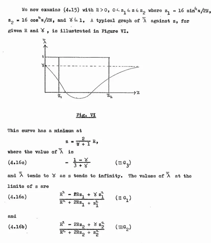
must be minimised as a function of r (70), ^ w < mas

To effect this minimisation, we consider the function

G(%,r) t* , r> 0,

where 0 ^ a z L b#

40

BQ _{that the maximwa of |G(x,r)j ocoura at one of the end pointe of th#}

interval• Hence,

max |G(x,r)j * max

From Figure I, it ia easily aeon that

r - a r - b

r + a > r + b

r*»

max |0(x,r)| c\ t

0 - r~

b 4* r *

r - a r + a * where r* ia given by

b - r*

b + r- + ar% - a

that ii 3?^ «S

Thue, it follow© that

min f max. |G(x,r%) » (l(a,Alab)

V7Ô (3L>LkV> J

j[ab — a A’ab -f a

1 4* (a/b)^’

-1

Thuo, with a λ f 4* and b » f 4- (2oin^%/2H)~^,

(2*94) min %

1"7Ô 1 + - aln^iAl (1 + 2f +

Vov each permissible value of f, (2.24) gives the optimusn convergence

factor, and tlio value of r nooooaary to achieve this optimum convergence is

(2.25) • r* - (1 V 2f f'^sinH/g)'44ln'-u/H .

X , <2\

■V /L1'“’^ ; r-i'r^or^ \ z: ^ C^ 3"^

>r - T=*: -^^ypjiL\c;,\ - U

41

kept constant during the iterations# When r la allowed to var^ and

take the value r^ (1 &. 1 fox* each of m cuoceeoivo itoratione, the

situation is more complicated, This cace will he dloouGoed in the next

section of this chapter*

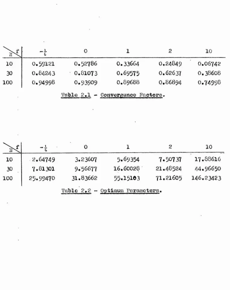
Returning to (2*24)$ it can ho seen that the optimum convergence

factor in unity when f » -(2c o g ^ a n d tends to %ero as f tende to

infinity* For k - 10, 30 and 100* the optimum conyergenco factors and

corresponding iteration parameters for various yalues of f within the

permissible range given by (2*23) ero shown in Tables 2.1 and 2*2

respectively, I'roia Table 2*1, we see that ,the beat convergence factor for a given value of B is obtained when f is positive and as largo as possible. In particular, the original r*R. method (f « 0) has a bettor

convergence factor than the optimuia formula (f »* derived previously

to solve (2*1),

The substantial improvement in convergence of the alternating direction method which arises frosa the choice of large positive values of the parameter f may, however, be accompanied by a certain loss of

acouraoy* The iteration procedure described by (2*21) reduces to

(s.86) (C. •;• - 0,

when u » » u ** u, for _{Ul4'X Ml} m sufficiently largo* however, equation (2*19)

can bo replaced by

K •*' • °»

kl

G 0 1 2 10

10 0*59121 0.52786 0.33664 0.24849 O.O6742

30 0,84243 0.81073 0.69575 0.62637 0.38608

100 _0*9499# 0.93909 0.89668 0.86894 0.74998

Table .2*1 - Oonvorfyenoo Faotor

«* *G _{0 1} 2 10

10 2*64749 3*23607 5,69354 7,50737 17.88616

30 7,81301 9,56677 16*60028 21.48524 44*96650

100 25,99470 31*83662 55,15103 71.21605 146*23423

correct to fourth-order dlffarunces, and so it follows from (2*26)

that equation (2,21) in moot accurate when f « - ^ , a result obtained

previously, and that there Id a loso of accuracy when f in largo. In

fact, ao f tends to infinity, equation (2,26) dogenerateo into

(8,2?) » 0,

(f

which ie no longer a difference approximation to Laplace's equation.

Accordingly a balance is required between tho rate of convergence (an optimum when f io infinite} and the accuracy of the procoso (an

optimum when f Howevex*, it will be shown in 11*11, by moans of

4^

II#10, ' lletliodà of Gelootln^ Beauenoee of Iteration Parameters#

If tho iteration parameter r in (2*22) io allowed to vary and

take the value (1 G 1L m) for each of m euccossivo itoratione, then

after tho la-th iteration the initial error at the node (c /\y) where

fift «si, 2, « » , B-1, will have been reduced by the factor

m

m t^i ^ ^ - v )

liÇTJTJ (r^ + V )

(2*28)

whore f 4 (2sin^^s.p/2B)'and f v (2sinS^q/2B) ' 1 kB-1,

lilquatlon (2*28) follows immediately from IX *9 * In or dor to obtain the

optimuia values of r_, r,^, r^$ • _{■jL cl 3} * , r _m, we must lainimiee

(r^ - /U-) - V )

(2.89)

L~l liX

(r^ + /i-T* ir^ + V

» max

cvkvLW

~ V ?! + Y

where r » (r^* v^f • • $ r,^) and a « f i (2cos^>t/2H ) b - f (2ein^ (/21l) I

The problem of minimising is equivalent to tho problem of determining

the rainimax of the rational functions involved over certain domains#

In this section, methods of obtaining tho optimum, or "good", that is, near optiîatuii, parameters for the model problem - the hirichlet

problem for a unit square - will be briefly summarised#

One choice of parameters, based on an idea of Peaceman and Haohford

46

(

2

.

30

)

whore u is tho oiaalleot integer euoh that

(

.

)

where b » ff2 - 1 * 0.414 * In practice, a number of cycleo of parameters

iB used until the error at every nod© is less than or equal to some

preasoigned quantity. It may be shown (Birkhoff et al

[

])

one cycle of Young's parametors,

1

-1 + (s/d5‘A.h

A similar choice of parameters was presented by Wachapross [45]

and Machspross and Habetler [46]* This parameter oequenoo is given by

(2.32) r. _a

i * 1, 2

where m is the smallest integer such that

(2.33) i,2(ia-l)

where, once more, b <« J2 - l « 0*414 ♦ After one cycle of these

parameters

1 - (a/b

1 + (a

’/Xm—â

e a t :

heithar of these choices results in optimum values of the parameters but they do give convergence rates not far froia the opticaun. Young

and Frank l"5lj have shown that tho bachopress parameters are a better ohoico than those of Young* Numerical experiments tend to confirm this

47

, WaobepreoG [4#] has devlsad an algorithm for calculating oxact

optimum parameters when the nwiiber of parameters 1b a power of 2. An independent proof of this algorithm was simultanoouclj given by Gastinei

(unpublished)* In experiments carried out by Young and Frank [51] and Birkhoff et al [3], there wao very little, if any, gain by using the optimvuijjparometerB inutoad of the WaohapreaG parameters* In a la tor paper, WaohspreGo 147], this algorithm is general!aod to the oaso in which the region under consideration is rectangular*

Recently, i)e Boor and Rice [10] have shown that the use of simple programming methods gives the optimuu parameters for all ra>l* Also, they devise a new parameter sequence which appears to be relatively easy to use and gives nearly optimua results*

The most recent method of choosing tho parameters is that devised by il*B*Jordan, who hao obtained an exact expression for the optimum

parameters in terms of Jacobian elliptic functions* From this expression, Jordan obtains other estimates of the parameters* His analysis ie

summarised in the Appendix of tJaohspreso [47]#

It was originally believed (Peacoman and Eachford [34]) that, for

an alternating direction method of type (2*22) to be convergent, the

parameter r had to be the same for both stepo of the iteration* However,

Pearcy [35] has shown that (2*22) is still convergent when the parameter

X l . i l . A D I M e t h o d s a n d i - i o n - E e o t a n ^ u l a r R a g i o n s »

It should bo omphaBisod that tho theory developed in tho previouG

oeotiono of this chapter for ADI methods only applies when tho operators

and h coiamuto, that ia, if and only if tho region under consideration

-A. y ■

io rectangular, (Birkhoff and Varga [2]), However, tho P#&, method has been used with considerable sucoeoo for the solution of tho five-point XiUplao© difference equation in cases where tho theory is known to be

inapplicable* (See Young and Ehrlioh [50], Price and Varga [36])# He

now investigate the posoibility of using (2.22) with f / 0 for the

Mrichlet problem on non-rectangular regions,

I/o observe that 0 difference approximation to Laplace's equation of

typo (2.26), with f / 0, that is, a difference approximation involving

nine points, can only be employed when the boundaries of the region under consideration are parallel to the coordinate axes, otherwise it

would involve a point outside the region when applied to tho nodes nearest to tho boundaries. Also, for a region with boundaries parallel to tho coordinate axoo other than a square or rectangle, formulae (2.22) do not directly yield the solution of Laplace's equation. This may be

soon by considering tho totality of difference equations of typo (2,26)

which gives rise to a system of linear equations of the form

% - £ »

where u ie tho vector of the unknoims u. . and g io a constant vector_{**" 1,3}

arising from the boundary values. Writing (2.22) in matrix form, we

4s

, [I, + i(r + f

= [I - i(p - f)V]u^ + i(r +, f)g

[I + i(r +

= Cl - i(r -

+ i(r - f)g ,

where H and V are matrices which are such that if [Hu](x^,y^) denotes

the component of the vector Hu corresponding to the mesh point then

CHu](x ,y^) . + 2u(x^,y^^) - u(x^+h,y^)

CVu](x^,y^j) = -u(x^,y^-h) + 2u(x^,y^) - u(x^,y^+h).

This method clearly converges to the solution of (H + V + fHV)u « £ ,

and only in the case of a square, or rectangle, is this the original set of equations, that is, A may he written in the form

A * H + V -kfHV

if and only if the region is a square or rectangle in which case, if A is an H X H matrix, H and V take the forms

H « H V = 21 -I

H -X 21 -I

1 -I 21 -X

* ♦

« •

H -X 21

respectively, where H is the M x H matrix

H s 2 - 1

-1 2 -1

go

and X is tho unit matrix.

As an example of a problem involving a region on which IÎ and V

(or and (T ) do not commute, consider the Diriohlet problem for the

region shown in Figure II, (see Varga [44] page 218, example 3), where the circled, numbered nodes are the unknowns*

©

-X-@ >r

Figure XI»

In this case.

A * 4(X+f) -(l+2f) -(l+2f) H ** 2 -1 0

-(l+2f) 4(l+f) f -1 2 0

-(l+2f) f 4(l+f) 0 0 2

? - 8 0 -Ï _{11 V 4 fHV «} ^— _{4(l+f) -(l+2f) -(l+2f)}

0 2 0 (l+2f) 4(l+f) f

-1 0 2 _{(l+2f) 0 4(l+f)}

from which it is obvious that

A / II + V + f HV

and hence tho ADI method (2*22) does not yield the solution of the

problem*

5-1

'boundarioî;', avo parallel to the axes in conjunction with the numorioal

alternating procedure of Miller [26], which io a numerical analogue of the Uchwara alternating procedure, (Kantorovich and Krylov [22]). This procedure enables on© to solve the Biriohlet problem for Laplace*o

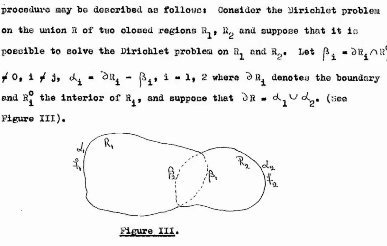
equation on tho union of two overlapping plane regions, provided that the hirichlet problem can be solved on each separately, and that their boundaries intersect at non-s«ro angles* The numerical alternating, procedure may be described as followsi Consider the Biriohlet problem

on the union H of two closed regions and suppose that it is

possible to solve the Biriohlet problem on IL and %_* Let_{X «■-'f { X 1}

/ 0, i / j, çk^ m ₁ « 1, 2 where ^ denotes the boundary

and hJ the interior of H^, and suppose that ol^* (#ee

Figure III).

Figure XIX.

Let us consider a fixed Biriohlet problem, with given boundary function f on c)U, and let u denote tho solution of the problem. Let i% be the

boundary function on which is the restriction of f to the external

arc cL that is, » f on * 0 on p^*

alternating procedure may be written as follows|

S’!

Lot be tho solution of LapXaoo^e equation on ly for

boundary values on and arbitrary values on

let u^(x#y) be the solution of laplaoe'g equation on for

boundary values on and u^p^(2c,y) on n » 1, 2, • • . |

let u^(x,y) bo the solution of Laplace's equation on for

boundary values on and uj(x,y) on n * 0, 1, 2, , , , .

Miller [26] shows that vu_^ converges on ÏL_il» and u!? oonvergos on_d-f

to tho solution u of Laplace's equation on H for boundary values f on Thus, if the region under consideration is the union of two over­

lapping rectangles end IL, we may employ the ADI method (2.22) to

solve Laplace's equation (2*19) on This method may extended

to cover the case of three or more overlapping regions, and, also, there io no need to restrict the region to two dimensions*

Tho solution of Laplace's equation on an L-shaped region by ##r0ot

application of the ADI method (2*22) with f « 0 and in conjunction with

S3

T T 1 O

ft# «f.-# Q •Footnote.

Originally, the formulae occurring in this chapter and In the paper

by Mitcholl and Fairweather [30] were not oxpresaed in terras of central

differences but in terms of a network of nodal points, which were nuiiibored, an illustrated in Figure XV, for eaoo of reference. In

Figure IV*

particular, the gener&liaed formula (2*7) vac written in the form

(2*34) h;[ (u0 + all + bX) 4* (oUg + dV. •+• ef»)] 0

where

IJ « ^16 '*18 **19 4*“21

X « _{“I* **17 f “20}

Y # ^10 **12 4- **13 4"“15

**3 4" '^11 4* "14

end k, a, b, o, d and e are functions of r* In order that this formula be written ao a pair of F.ii. or I)*R* type formulae, the conditions

b^ •» a and e • » od or simply b^ « a must be aatisfied respectively# The

optimum formula (2*10) was obtained by expanding Iv, Y, K, Z _as