scattering setup
.
White Rose Research Online URL for this paper:
http://eprints.whiterose.ac.uk/126471/
Version: Accepted Version
Article:
Fahimi, Z, Aangenendt, FJ, Voudouris, P et al. (2 more authors) (2017) Diffusing-wave
spectroscopy in a standard dynamic light scattering setup. Physical Review E, 96 (6).
062611. ISSN 2470-0045
https://doi.org/10.1103/PhysRevE.96.062611
(c) 2017, American Physical Society. This is an author produced version of a paper
published in Physical Review E. Uploaded in accordance with the publisher's self-archiving
policy.
[email protected] https://eprints.whiterose.ac.uk/ Reuse
Unless indicated otherwise, fulltext items are protected by copyright with all rights reserved. The copyright exception in section 29 of the Copyright, Designs and Patents Act 1988 allows the making of a single copy solely for the purpose of non-commercial research or private study within the limits of fair dealing. The publisher or other rights-holder may allow further reproduction and re-use of this version - refer to the White Rose Research Online record for this item. Where records identify the publisher as the copyright holder, users can verify any specific terms of use on the publisher’s website.
Takedown
If you consider content in White Rose Research Online to be in breach of UK law, please notify us by
Zahra Fahimi,1, 2 Frank Aangenendt,1, 2, 3 Panayiotis Voudouris,1, 2 Johan Mattsson,4 and Hans M. Wyss1, 2, 3,∗ 1Department of Mechanical Engineering, Materials Technology,
Eindhoven University of Technology, Eindhoven, the Netherlands
2Institute for Complex Molecular Systems, Materials Technology,
Eindhoven University of Technology, Eindhoven, the Netherlands
3Dutch Polymer Institute (DPI), Eindhoven, the Netherlands
4School of Physics and Astronomy, University of Leeds, Leeds, United Kingdom
(Dated: December 6, 2016)
Diffusing-Wave Spectroscopy (DWS) extends dynamic light scattering measurements to samples with strong multiple scattering. DWS treats the transport of photons through turbid samples as a diffusion process, thereby making it possible to extract the dynamics of scatterers from measured correlation functions. The analysis of DWS data requires knowledge of the path length distribution of photons traveling through the sample. While for flat sample cells this path length distribution can be readily calculated and expressed in analytical form, no such expression is available for cylindrical sample cells. DWS measurements have therefore typically relied on dedicated setups that use flat sample cells. Here we show how DWS measurements, in particular DWS-based microrheology measurements, can be performed in standard dynamic light scattering setups that use cylindrical sample cells. To do so we perform simple random walk simulations which yield numerical predictions of the path length distribution as a function of both the transport mean free path and the detection angle. This information is used in experiments to extract the mean-square displacement of tracer particles in the material, as well as the corresponding frequency-dependent viscoelastic response. An important advantage of our approach is that by performing measurements at different detection angles, the average path length through the sample can be varied. Using measurements on a single sample cell, this gives access to a wider range of length and time scales than obtained in a conventional DWS setup. Such angle-dependent measurements also offer an important consistency check, as for all detection angles the DWS analysis should yield the same tracer dynamics, even though the respective path length distributions are very different. We validate our approach by performing measurements both on aqueous suspensions of tracer particles and on solid-like gelatin samples, for which we find our DWS-based microrheology data to be in very good agreement with rheological measurements performed on the same samples.
PACS numbers: 47.57.-s, 46.35.+z, 78.35.+c, 07.60.-j
I. INTRODUCTION
Since its development in the 1980’s, Diffusing-Wave Spectroscopy (DWS) [1–3] has proven to be an important and versatile tool for studying the dynamics, mechanics and structure of a wide range of soft materials. [4–11] By taking advantage of the fact that the transport of photons through an optically turbid sample can be de-scribed as a diffusion process, DWS extends Dynamic Light Scattering (DLS) measurements to the highly mul-tiple scattering regime. It thus enables access to the dynamics of a material at very short time and length scales. The method is particularly useful when combined with the concept ofmicrorheology, where information on the dynamics of tracer particles added to a material are used to extract information on the material’s viscoelas-tic properties. [12–16] However, the proper analysis of any DWS measurement requires detailed knowledge of the path length distribution P(s) for photons traveling
∗Electronic address: [email protected]; URL: http://www.mate.
tue.nl/~wyss
through the sample to the detector. For a number of sam-ple geometries and experimental situations, the calcula-tion or estimacalcula-tion ofP(s) has been described in previous studies, including for the situation of backscattering from a flat sample cell of infinite thickness, or for transmission through cone-plate cells or flat circular cells of finite di-ameter and thickness. [9, 17, 18] Importantly, for sample cells in the shape of a flat slab of thicknessL, infinitely extended in height and width,P(s) can be expressed in analytical form, and the analysis of DWS data is there-fore straightforward. [3, 17]
For the cylindrical sample cells used in conventional dy-namic light scattering setups, however, an analytical ex-pression forP(s) is not available. DWS measurements are therefore usually performed in dedicated instruments that use flat sample cells.
In this paper, we show how DWS-measurements can be performed in a standard dynamic light scattering setup, using cylindrical sample cells. We perform simple numer-ical random walk simulations to account for the propa-gation of photons through a cylindrical cell and describe how this information is used to obtain the mean-square displacement of tracer particles from the temporal au-tocorrelation functions determined in experiments. We
further show that by performing measurements at dif-ferent detection angles, the range of accessible time and length scales can be extended; this is in analogy to stan-dard DWS measurements employing a range of different cell thicknesses. Importantly, our approach also provides a valuable consistency check, especially in the context of microrheology, since measurements taken at different detection angles should yield the same viscoelastic re-sponse, even though the corresponding correlation func-tions must be very different due to the variation in ge-ometry and average path length.
In analogy to a conventional DWS measurement, the transport mean free pathl⋆is determined by a calibration
measurement on tracer particles of well known uniform size, suspended in a Newtonian liquid of known viscos-ity; the expected single particle dynamics is thus known
a priori. Alternatively, the transport mean free path can also be directly determined from the measured scatter-ing intensity as a function of angle, I(θ) if an initial experimental calibration is combined with results from our simple numerical calculations. In the highly multiple scattering limit, and in the absence of absorption in the sample,I(θ) is well approximated by a function that de-pends only on l⋆, on the corresponding calculated path
length distributionP(s), and on a constant βexp that is
determined by the experimental setup.
We thus demonstrate that standard goniometer light scattering setups can be successfully used for DWS mea-surements. Compared to dedicated DWS setups, our method has the advantage of being able to reliably deter-mine the transport mean free pathl⋆as well as to extend
the range of accessible length and time scales, using only a single cylindrical sample cell.
We illustrate and test the use of our approach by per-forming DWS-based microrheology measurements on a typical solid-like soft material, gelatin, and find the re-sulting frequency-dependent viscoelastic moduli to be in very good agreement with separately performed rheolog-ical measurements.
II. EXPERIMENTAL: MATERIALS AND
METHODS
A. Background on DLS, DWS, and microrheology
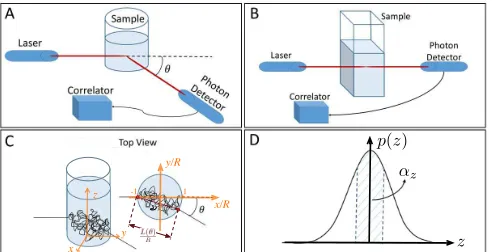
Standard static and dynamic light scattering experi-ments are limited to samples that exhibit very little mul-tiple scattering, with the overwhelming majority of de-tected photons having been scattered only a single time within the sample. A typical setup for such single scat-tering experiments uses a cylindrical sample cell that is il-luminated by a laser, as shown schematically in Fig.1(A). The detector, typically comprising an optical fiber that is coupled to a photomultiplier tube, can be positioned at a range of detection anglesθ, corresponding to scattering wave vectorsq(θ) = 4πnλ sin(θ/2), where n is the refrac-tive index of the sample and λis the wavelength of the
1 x/R y/R
-1 z
x y
FIG. 1: (Color online) Schematic experimental setup for typ-ical dynamic light scattering measurements. (A) Standard dynamic light scattering(DLS) setup employing a cylindrical sample cell and a goniometer, which enables accessing dif-ferent scattering anglesθ. (B)Diffusing-Wave Spectroscopy (DWS) setup in transmission geometry. The pathways of pho-tons are well-described by a random walk of step sizel⋆. (C)
Schematic of random walk simulations in a cylindrical geome-try. The detection angleθis defined as for conventional DLS; here it determines the distanceL(θ) between the points of en-try and exit of detected photons. (D)Expected distribution
p(z) of thezcoordinate where a photon exits the cylinder; a fractionαz (marked area) reaches the detector.
laser in vacuum. For single scattering, the fluctuations in the detected intensity, which reflect the dynamics of the scatterers, are then quantified by the temporal intensity autocorrelation function
g2(t) =
< I(˜t+t)I(˜t)>˜t < I(˜t)>˜t
2 , (1)
wheretis the lag time and the brackets< .. >˜tindicates
a time-average over all times ˜t. The field autocorrelation functiong1(t), measured at a wave vector q, reflects the
temporal fluctuations of the electric field. It can be re-lated, via the so-called Siegert relation to the intensity correlation function, asg1(t)≈
p
(g2(t)−1)/β, whereβ
is the coherence factor, [19] a constant that depends on the experimental setup. For a Gaussian distribution of displacements ∆r, the field correlation function g1(t) is
directly linked to the dynamics of scatterers in the sam-ple, as
g1(t) =e− q2
6h∆r 2
(t)i, (2)
where
∆r2(t)
is the time-dependent mean-square displacement of scatterers in the material. For the sim-plest example, where the scatterers are uniformly sized particles suspended in a Newtonian liquid, the particles undergo ideal Brownian motion, and thus
∆r2(t)
= 6Dt, whereD is the particle diffusion coefficient in 3 di-mensions. For this case, the field correlation function has a single exponential form, g1(t) = e−Γt, where the
q-dependent decay rate Γ =Dq2 is set byD.
[image:3.612.318.564.52.178.2]multiple scattering regime. A typical experimental setup for DWS is shown in Fig.1(B). In contrast to conven-tional DLS measurements, this technique requires that photons are scattered many times, before they reach the detector. For this highly multiple scattering regime, the propagation of photons through the sample can be ade-quately described as a simple diffusion process, where the details of each single scattering event are no longer rele-vant. This photon diffusion processes can be accounted for by a single parameter, the so-called transport mean free pathl⋆. This characteristic length scale is defined as
the average distance a photon travels in the sample be-fore its direction of propagation is randomized. The path of photons through the sample can thus be approximated as an ideal random walk with step sizel⋆. For such a
ran-dom walk the path length of photons, and the number of randomizing scattering events, is no longer uniform, as is the case for single scattering. Instead, the correla-tion funccorrela-tion measured in an experiment is determined by contributions from all path lengthssweighted by the path length distributionP(s), as
g1(t) = Z ∞
0
P(s)e−k0
2
3 h∆r 2
(t)is/l⋆
ds, (3)
wherek0= 2πn/λis the magnitude of the photon wave
vector in the sample ands/l⋆reflects the number of
ran-domizing scattering events experienced by a photon with path lengths. [3] The basis for this simple form of Eq.3 is that each of the approximatelys/l⋆randomizing
scatter-ing events contributes to a change of this particular pho-ton path by a squared distance of
∆r2(t)
, leading to a partial decorrelation ofg1(t). The cumulative
decorre-lations from all these randomizing scattering events thus lead to the functional form in Eq.3. Knowledge on the path length distributionP(s) is therefore essential in the analysis of DWS measurements; without such knowledge the measured correlation functions cannot be related to the dynamics of the scatterers. The path length distri-bution depends sensitively on the geometry of the sam-ple cell used in the experiment. For samsam-ple cells in the shape of a flat slab, infinitely extended in both height and width,P(s) can be expressed in analytical form as a func-tion ofl⋆ and the thicknessLof the sample cell. [3, 17] This is one of the main reasons why DWS measurements have typically relied on measurements performed in ded-icated instruments, employing flat sample cells.
Such dedicated DWS instruments can also offer other important advantages, in particular for measurements on solid-like, nonergodic samples, where the measured, time-averaged correlation functions are not representative of the ensemble-averaged dynamics of the sample. [20] Methods for acquiring ensemble-averaged correlation functions in DWS measurements include the use of double-cell techniques, where either an ergodic sample with slow dynamics [21] or a slowly rotating opaque disc [22] is placed in front of the sample cell. Both these techniques create a slow randomization of the incoming
photon paths, resulting in an ensemble-averaging of the collected temporal correlation functions. Either transla-tions of the sample cell or rotatransla-tions of an opaque disc can also be employed for ensemble-averaging using echo techniques, [23] yielding ensemble-averaged correlation functions at long time scales and with excellent statis-tics. [22, 24] While these ensemble-averaging techniques could in principle also be incorporated into a standard goniometer setup, we choose an alternative method, so-calledPusey-averaging. This method uses the measured time-averaged correlation function and the measured ensemble-averaged scattered intensity together with a simple theoretical treatment to provide the ensemble-averaged correlation function. [25, 26]
The ensemble averaged scattering intensityhIiecan be
readily acquired in separate intensity measurements dur-ing which the sample is rotated; the measured dynamics is perturbed by the motion of the sample, but the average scattering intensity is still properly ensemble-averaged. Using the ratio of the ensemble-averaged to the time-averaged scattering intensities Y = hIie
hIit, the
ensemble-averaged field autocorrelation functiong1(t) can then be
estimated as a function of the time-averaged correlation function as
g1(t) =
Y −1
Y +
1
Y
˜
g2(t)−σ2 1 2
, (4)
where ˜g2(t) = 1 + g2(tβ)−1 is the time-averaged
inten-sity autocorrelation function normalized by the coherence factorβ, which is obtained from the separate ensemble-averaged measurements, andσ2= ˜g
2(0)−1 characterizes
the short-time intercept of ˜g2(t).
We can now use the resulting ensemble-averaged field autocorrelation function g1(t) to extract viscoelastic
properties of the sample, using the microrheology con-cept [7, 12]. To do so, we employ the local power-law approximation developed by Mason et al [15, 16]. In brief, the method is based on the assumption that the Stokes-Einstein relation, which links the thermal motion of particles in a Newtonian liquid to the viscosity of the surrounding liquid, can be generalized to viscoelastic ma-terials with frequency-dependent linear viscoelastic mod-uli. The approximation also neglects inertial effects on the motion of the probe particles, which is justified for most soft materials at frequencies below≈1 MHz.
By describing the time-dependent mean square dis-placement as a local power-law around each data point, the magnitude of the frequency-dependent complex mod-ulus can be expressed in analytical form as
|G⋆(ω)| ≈ πa kBT
h∆r2(1/ω)iΓ(1 +α(1/ω)), (5)
where a is the particle radius, kBT the thermal
en-ergy,α(t) = ∂ln(h∆r
2 (t)i)
∂ln(t) is the logarithmic slope of the
B. Sample preparation
Polystyrene particles (micromod Partikeltechnologie GmbH, Germany) coated with a grafted layer (Mw =
300 g/mol) of poly(ethylene glycol) were used as tracer particles in the DWS measurements. The diameter of the particles is 1 µm and they are provided suspended in water at a concentration of 5 wt%. The test samples with tracers in water are prepared by mixing the stock particle suspension with deionized water (Milli-Q water,
σ > 18MΩ·cm at 25 C), to obtain the desired tracer particle concentrationsCtracer. To study the effect of the
transport mean free path l⋆, which is expected to scale
as l⋆ ∝ 1/C
tracer, we prepare a series of samples with
particle concentrations ranging from Ctracer ≈0.3 wt%
to 5 wt%.
The aqueous gelatin gel is prepared by mixing water with 5 wt% gelatin powder (type A, from porcine skin, Sigma, USA) and 1.25 wt% of tracer particles at elevated temperatures of ≈ 60◦C. The mixture is homogenized
for 30 minutes using a magnetic stirrer, transfered to the cylindrical sample cell used in the experiment, and subsequently allowed to cool down to room temperature.
C. Light scattering experiments
All dynamic light scattering experiments are per-formed in a static and dynamic light scattering setup (ALV CGS–3, ALV GmbH, Germany), equipped with a 50 mW solid state laser (λ = 532 nm) and a goniome-ter that allows for variation of the detection angle from
θ≈20 deg toθ≈160 deg. Measurements are performed in cylindrical cells with outer diameter 10 mm and inner diameter 8.65 mm; the cell radius relevant to the propa-gation of photons in the sample cell (see Fig.1(C)) is thus
R ≈4.33 mm. Measurements of 30 s duration are per-formed at detection angles between 30 deg and 150 deg in steps of 10 deg. To minimize the detection of stray light, reflected from surfaces in the setup, our measure-ments are performed in vertical-horizontal mode, with the incoming light vertically polarized and a horizontal polarizing filter placed in front of the detector.
For the gelatin samples we use separate experiments on the same sample to determine the ensemble-averaged scattering intensities hIie as well as the coherence
fac-tor β needed for the Pusey averaging method. In these separate experiments the sample cells are slowly rotated during data acquisition; we perform three such measure-ments at each scattering angle, each lasting 10 seconds.
In principle, the light scattering measurements we de-scribe in this paper could be performed with any stan-dard goniometer setup; however, not all laser sources that are included in standard goniometer setups may be suitable for performing DWS measurements. In partic-ular, as a result of the long path lengths of the pho-tons through the sample, DWS requires a laser source with a sufficiently long coherence length. Information
on the coherence length of a laser is difficult to obtain from the standard information provided by manufactur-ers, and its measurement requires complex setups only available in specialized optics laboratories. Within the range of concentrations studied here, the longest relevant path lengths of photons through the samples were limited to around 3 meters. This would be a problem for instance if a Helium-Neon laser were used, which has a typical co-herence length of only around 20 cm. Semiconductor lasers, and lasers coupled into single mode fibers, how-ever, typically have much longer coherence lengths that can reach hundreds of meters. While we have not directly measured the coherence length of our laser source, the good agreement of our path length simulations with ex-periments(see Results section) makes us confident that in our setup the coherence length of the laser is larger than the relevant path lengths of photons traveling through the sample.
III. RESULTS AND DISCUSSION
A. Simulation of photon paths through the sample
To properly interpret experimental data in a setup with a cylindrical cell, the path length distributionP(s) of photons traveling through the sample is required both as a function of the detection angleθand the transport mean free pathl⋆.
To achieve this, we perform numerical simulations of photons traveling through a cylindrical cell, assuming that they undergo an ideal random walk with step sizel⋆.
In the 2-dimensional coordinate system given in Fig.1(C), photons are released at point (x/R=−1 +l⋆/R, y/R=
0), wherel⋆is the transport mean free path andRis the
radius of the cylindrical cell. Subsequently, each photon is propagated in steps ofl⋆/R, where each step proceeds
in a random (3D)-direction. At the point where the pho-ton exits the cell (x2+y2> R2), we evaluate the number
M of scattering events, and record the detection event with respect to the observed detection angleθ.
We do this by dividing the surface of the cylindrical cell into nbins angular bins, spanning from 0 to 180 deg
(taking into account the symmetry around the x-axis). In addition, to take into account the 3-dimensional na-ture of photon transport in the real geometry, we consider the fact that each realization of a 2-dimensional photon path represents a whole range of possible 3-dimensional paths with an identical number of scattering events M
and identical (x, y)-paths. Since in the z-direction the photon also performs a (1-dimensional) random walk, we can readily express the probability distribution p(z) for the photon to end up at a positionz after propagating
M random steps. What is relevant here is the fraction of those paths that will reach the detector, as illustrated in Fig.1(D). We assume that all photons with|z|<∆z
are detected; in accord with the resolution of the angu-lar bins, we set ∆z = π
10
-210
-110
0s
[m]
10
-210
-110
010
110
2P
(
s
)
A
l⋆/R=0.01
l⋆/R=0.02
l⋆/R=0.04
l⋆/R=0.08
l⋆/R=0.16
10
-110
010
1s/
s
˜
10
-210
-110
0P
(
s
)
·
˜
s
[m
]
B
l⋆/R=0.01
l⋆/R=0.02
l⋆/R=0.04
l⋆/R=0.08
l⋆/R=0.16
10
-210
-1l
⋆/R
10
-210
-110
0˜
s
[m
]
C
fit: exponentm=-0.975
10
-110
0L
(
θ
)
/R
10
110
210
310
410
5˜
s/l
⋆
D
l⋆/R=0.01
l⋆/R=0.02
l⋆/R=0.04
l⋆/R=0.08
l⋆/R=0.16
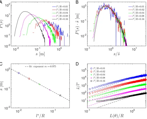
FIG. 2: (Color online) Simulation results. (A)Path length distributionP(s) for different values ofl⋆/R, calculated at a fixed
detection angleθ= 90 deg. (B)Master curve of scaled path length distributions, showing that the shapes ofP(s) calculated at differentl⋆/Rare similar. (C)Corresponding average path lengths ˜sas a function ofl⋆/R. As expected, we find a scaling
˜
s ∝1/l⋆, as indicated by a power-law fit to the data (dashed line), yielding an exponent m=−0.975±0.05. (D)Average
number of scattering events ˜s/l⋆as a function of the distanceL(θ) between the entry and exit points of the detected photons.
The dashed lines serve as a visual reference, indicating the scaling ˜s/l⋆∝L(θ)2 that would be expected for an unrestricted
random walk.
contributing 3-dimensional paths is given as
αz= erf( 3∆z
l⋆√M), (6)
where erf is the error function, and
q
l⋆2/3 is the
effec-tive 1-dimensional step size in the z-direction. We thus account for diffusion in thez-direction in our statistics of path length distributions by, instead of adding 1, adding a contribution αz to the angular bin corresponding to
each simulated photon path: f(nbin)→f(nbin) +αz.
Each bin thus represents a detection area of surface areaAbin≈
πR nbin
2
. The cumulative value of each
angu-lar bin, after propagatingN photons and normalizing by
N, thus defines a (dimensionless) scattering intensity as
Isim:= f(n bin)
N , representing the probability for a photon
to reach the detection area corresponding to bin number
nbin.
In addition to recording the angle where the photons end up, we also record, for each angle θ(nbin), a
distri-bution of the number of scattering events, by adding a contribution αz to a bin accounting for the number of
scattering events at each angleθ(nbin). The bins are
lin-early spaced, with bin number 100 representing a num-ber of approximately (L(θ)/l⋆)2
[image:6.612.58.562.51.457.2]and the detection point of the photons.1 We use 300
bins per angleθ(nbin), thus accounting for up to 3 times
the expected typical number of scattering events; higher numbers, while not counted, in practice are extremely rare in our simulations and do not significantly affect the resulting path length distributions.
In order to achieve good statistics in the calculated path length distributions, the paths for a large number of photons have to be simulated.
In the actual experiments obtaining good statistics is usually not a problem, due to the enormous number of photons that are propagated. In our experiments we use a laser with 50 mW of power at a wave length of 532 nm; this corresponds to≈1017 photons entering the sample
cell, every second. Such numbers are beyond the capabil-ity of computer simulations; in comparison, for our cal-culations we typically simulate 109 photons propagating
through the sample, which is enough to yield reasonable statistics, and relatively smooth calculated path length distributions.
B. Scaling properties of P(s)
Typical obtained simulation results forP(s) are shown in Fig.2(A); these curves are calculated at a fixed angle
θ = 90 deg for different values of l⋆/R. Interestingly,
while the average path length decreases with increasing
l⋆, the shapes of these path length distributions appear
surprisingly similar, .
In fact, we can overlay the curves from Fig. 2(A) and create a master curve, as shown in Fig. 2(B). To obtain this master curve, we have rescaled the path length with a factor ˜s and multiplied the magnitude with the same factor; it turns out that ˜s is the average path length, defined below in Eq. 7.
Any practical use of the calculated path length dis-tributions requires that P(s) data are available for any arbitrary value ofl⋆. To address this problem, we
calcu-late path length distributions for different values ofl⋆/R
and examine the scaling properties of these path length distributions.
In contrast to an ideal random walk, the path of pho-tons through our cylindrical sample is constricted by the geometry. Nevertheless, the essential scaling properties of a random walk still hold approximately for the path length distributions simulated here. In particular, for an unrestricted random walk of step size l⋆, we expect
the mean square displacement
∆R2
to be given as
∆R2
=M l⋆2, with M the number of steps.
Consider-ing the average path length
1 In the cylindrical cells studied here, the average pathlengths ˜s depend on the detection angle and are typically shorter than estimated from ˜s/l⋆
≈(L(θ)/l⋆)2, as seen in Fig.2(B).
˜
s:=
Z ∞
0
sP(s)ds , (7)
we can estimate the average number of scattering events ˜M to travel to a point at distanceL(θ) from the origin to be approximately given as ˜M ≈(L(θ)/l⋆)2
, as would be the case for a completely unrestricted random walk.
As the path length iss=M l⋆, the average path length
should scale with L(θ) and l⋆ as ˜s ≈ L(θ)2/l⋆.
Con-versely, at fixed detection angleθand thus fixed distance
L(θ), we would clearly expect a scaling of ˜s∝1/l⋆.
To test this scaling, we examine the P(s) data with respect to both l⋆ and the detection angle θ, where a
variation of the latter corresponds to a variation of the distanceL(θ) between the entry and detection points of the photons. In Fig.2(C) we plot the average path length ˜
sas a function ofl⋆/R, for simulation data calculated at
a single detection angle θ = 90 deg. Indeed, the data is in excellent agreement with a scaling of ˜s ∝ l⋆−1
; the dashed line in Fig.2(C) shows a power-law fit to the data, yielding an exponent of−0.975±0.05. This scaling is a consequence of the self-similarity of random walks, which enables us to approximate each random walk with a “coarse grained” version of larger step size; this scaled random walk essentially follows the same path, but, as a result of the increased step size, exhibits a reduced con-tour length.
In contrast to this simple scaling as a function of l⋆,
if we examine the average number of scattering events as a function ofL(θ), we find significant deviations from the na¨ıvely expected scaling ˜s/l⋆ ∝ L(θ)2, as shown in
Fig.2(D). The symbols in this figure show the simulation data for different values of fixedl⋆/R, and the solid lines
show the simple prediction discussed above, a power-law with exponent 2. In hindsight, it is clear that such de-viations should be expected, as, in contrast to the l⋆
-dependence at fixed detection angle, a variation ofL(θ) implies a significant modification of the effective sample geometry. It is thus evident that calculations of P(s) at different detection angles are necessary. However, the simple scaling properties with respect tol⋆, highlighted in
Fig.2(B), can be exploited to obtain accurate path length distributions for arbitraryl⋆-values, based on simulations
performed at a single value ofl⋆/R.
C. Determination of l⋆ for samples with known
tracer dynamics
Typically, when DWS experiments are used to perform microrheology measurements, uniformly sized tracer par-ticles are added to the soft material of interest. If the transport mean free path l⋆ is known, the dynamics of
50 100 150
Detection angle
θ
[deg]
10-4 10-3
F
it
te
d
l
⋆[m
]
G
φ= 0.313%
φ= 0.45%
φ= 0.625%
φ= 0.9%
φ= 1.25%
φ= 1.65%
φ= 2.5%
10-3 10-2
Volume fraction
φ
10-4 10-3
F
it
te
d
l
⋆[m
]
H
θθ= 30 deg= 40 degθ= 50 deg
θ= 60 deg
θ= 70 deg
θ= 80 deg
θ= 90 deg
θ= 100 deg
θ= 110 deg
θ= 120 deg
θ= 130 deg
θ= 140 deg
θ= 150 deg
10-7 10-5 10-3
t
[s]
0 0.2 0.4 0.6 0.8 1g
1(
t
)
A
exp. (φ= 0.625%) sim. (l⋆= 540µm)
10-7 10-5 10-3
t
[s]
0 0.2 0.4 0.6 0.8 1g
1(
t
)
B
exp. (φ= 0.625%) sim. (l⋆= 531µm)
10-7 10-5 10-3
t
[s]
0 0.2 0.4 0.6 0.8 1g
1(
t
)
C
exp. (φ= 0.625%) sim. (l⋆= 521µm)
0 2 4 6
t
[s]
×10-4-3 -2 -1 0
ln
(
g
1(
t
))
D
exp. (φ= 0.625%) sim. (l⋆= 540µm)
0 2 4 6
t
[s]
×10-4-3 -2 -1 0
ln
(
g
1(
t
))
E
exp. (φ= 0.625%) sim. (l⋆= 531µm)
0 2 4 6
t
[s]
×10-4-3 -2 -1 0
ln
(
g
1(
t
))
F
exp. (φ= 0.625%) sim. (l⋆= 521µm)
∼1/φ
Mie theory
θ=50 deg θ=90 deg θ=150 deg
θ=50 deg θ=90 deg θ=150 deg
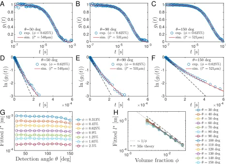
FIG. 3: (Color online) Simulation results versus experiments for colloidal particles in water (φ= 0.625%,d= 1µm): Measured (blue circles) and calculated (red line) field correlation functiong1(t) for a detection angle ofθ= 50 deg(A),θ= 90 deg(B),
and θ= 130 deg (C). ln(g1(t)) as a function oftfor the same values ofθ = 50 deg(D),θ = 90 deg(E), and θ= 130 deg (F).(G):l⋆obtained from fitting simulation data to experiments, as a function ofθ for differentφ. (H): The samel⋆ values
plotted as a function ofφfor different values of the detection angle θ; we find approximatelyl⋆∝1/φ, as illustrated by the
dotted line. The data is also in fair agreement with predictions from Mie scattering theory,[27–29] shown as a dashed line.
50 100 150
Detection angle
θ
[deg]
100 101 102 103
I
ex p[k
Hz
]
B
l⋆/R= 0.035
l⋆/R= 0.05
l⋆/R= 0.063
l⋆/R= 0.085
l⋆/R= 0.118
l⋆/R= 0.159
l⋆/R= 0.218
50 100 150
Detection angle
θ
[deg]
10-11 10-10 10-9 10-8 10-7
I
sim[ar
b
.
u
n
it
s]
A
l⋆/R= 0.01
l⋆/R= 0.02
l⋆/R= 0.04
l⋆/R= 0.08
l⋆/R= 0.16
10-1 100
l
⋆/R
101 102 103
I
ex p,
β
ex p·
I
sim[k
Hz
]
C
θ= 150 deg
θ= 140 deg
θ= 130 deg
θ= 120 deg
θ= 110 deg
θ= 100 deg
θ= 90 deg
θ= 80 deg
θ= 70 deg
θ= 60 deg
θ= 50 deg
θ= 40 deg
θ= 30 deg
FIG. 4: (Color online) Obtainingl⋆from intensity measurements: Calculated and measured intensities as a function ofθ and
l⋆. (A) Intensity as a function of θ for simulations employing different values of l⋆. (B) Concentration dependence of the
[image:8.612.88.555.57.396.2] [image:8.612.57.562.496.649.2]surrounding material area priori known, thenl⋆ can be
extracted from a DWS measurement. A requirement is that the particles scatter much more strongly than the material, ensuring that any detected dynamics are re-lated only to the particle dynamics, and not to fluctu-ations within the surrounding sample. If this criterion is fulfilled, the simplest method for determiningl⋆ is to
measure the scattering of uniformly sized, spherical par-ticles, suspended in a Newtonian background liquid of known viscosity.
To test our approach, and for calibration of the trans-port mean free path l⋆, we here perform a series of
ex-periments using samples with different concentrations of uniformly sized polystyrene particles (coated with poly-ethylene glycol, Mw ≈300 g/mol, 1µm diameter,
pur-chased from micromod GmbH, Germany) suspended in water. We measure the field autocorrelation function
g1(t) of the scattered light for these samples and test
how the correlation functions predicted from our pho-ton path simulations compare to these experimental data. As shown in Fig.3(A-C), where we show data on a sus-pension of particles at a volume fraction φ = 0.625% and detection angles θ = 50 deg, 90 deg, and 130 deg, we obtain remarkably good agreement between exper-iments (shown as blue circles) and simulations (shown as red lines), where l⋆ is the only adjustable
parame-ter. While the dynamics is expected to be purely Brow-nian, with
∆r2(t)
increasing linearly with timet, due to the broad path length distribution of photons passing through the sample,g1(t) deviates significantly from the
single exponential decay that would be observed in single scattering experiments. This can be more clearly seen in Fig.3(D-F), where ln(g1(t)) is plotted as a function
of time; in such a plot an exponential decay would ap-pear as a straight line, as illustrated by the dashed lines, which show exponential fits to the short-time regime of
g1(t). The non-exponential shape of the data thus
be-comes evident and is captured very well by the curves predicted from our simulations, shown as red lines. Fits performed for the same sample, but at different angles, should yield the samel⋆-values. Indeed, we obtain good
agreement between thel⋆-values extracted from the data
in Fig.3(A-C): we obtainl⋆= 540µm,l⋆= 533µm, and l⋆= 523µm at angles ofθ= 50 deg, 90 deg, and 130 deg, respectively. In fact, we obtain good agreement between measurements taken at different angles for all the con-centrations studied, with volume fractions ranging from
φ = 0.313% to 2.5%. As shown in Fig.3(G), the fitted
l⋆-values as a function ofθexhibit only small variations.
Somewhat larger deviations are observed for the sample with the lowest concentration, at the largest detection angles. We attribute this to the fact that this sample has the longest l⋆, combined with the shortest distances L(θ) between entry point and exit point of the photons;
l⋆ ≈1 mm and L(θ)≈2.2 mm and thusL(θ)/l⋆ ≈2.2.
In this case the path length of photons is no longer ade-quately described as an ideal random walk.
Besides these discrepancies at small values of L(θ), the
fitted l⋆-values depend only on the volume fraction,
ir-respective of the detection angle. To examine the φ -dependence of the data, in Fig.3(H) we plotl⋆as a
func-tion ofφ, observing approximately the expected scaling
l⋆ ∝1/φ, [30] as indicated by the dotted line. The data
is also in fair agreement with Mie scattering calculations plotted as a dashed line in Fig.3(H). [28, 29] The calcu-lations are performed using the web application available on the website of LS Instruments, Switzerland, [27] using as input parameters the particle size, the wavelength of the laser λ = 532 nm, as well as a refractive index of
nPS= 1.598 for the particles andnH2O= 1.33 for water.
D. Obtaining l⋆ from intensity measurements
In the absence of absorption, the intensity detected at each angle should be fully determined by the trans-port mean free path of photons in the sample. While absorption is relatively straightforward to include in the current data analysis, here we choose to neglect its ef-fects since absorption is relatively weak in the aqueous samples studied; the typical absorption length is much longer than the typical path length of photons through the samples. As a result, after calibration using a refer-ence sample of known dynamics, a simple measurement of the scattering intensity at different angles on the sam-ple of interest is sufficient for determining itsl⋆. To
vali-date this, we compare the scattering intensities predicted from the simulations with those measured in experiments performed on our polystyrene suspensions.
In Fig.4(A) we plot the scattering intensity Isim as a
function of detection angleθ, as predicted from the pho-ton path simulations. The shape of these curves is very different from those typically obtained in single scatter-ing experiments on dilute suspensions, where generally the intensity is highest at small detection angles, corre-sponding to lowq−values. In the highly multiple scat-tering regime, however, the intensity is generally highest for detection points closest to the entry point of photons into the sample, which corresponds to largeθ-values.
Importantly, we find that the angular dependence of the recorded scattered intensity for the tracer particle suspensions agrees remarkably well with the behavior predicted from our simulations, as shown in Fig.4(B). For both simulations and experiments, we observe a ratio of
≈ 40 between the intensities measured at θ = 30 deg and θ = 150 deg. Moroever, comparing Fig.4(B) with Fig.4(A), we observe that the shapes of the simulated in-tensity curves are very similar to those of the experimen-tal data. In fact, the two data sets can be superposed simply by scaling the simulated curves with one single factorβexp, the value of which depends on experimental
parameters such as the size of the detection area, and the distance between the detector and sample. We find that good agreement between the measured and simu-lated curves is obtained for a value ofβexp ≈8·1010Hz,
Thus, given βexp, a good estimate of l⋆ can be
de-termined for a sample of unknown properties solely by measuring the scattered intensity at different angles.
E. Test on a viscoelastic material
Finally, we test the use of our method in the context of microrheology, where the measured correlation func-tions and the corresponding tracer particle mean-square displacements
∆r2(t)
are used for the determining vis-coelastic properties of a sample. As a test material we use a common solid-like soft material, an aqueous gelatin gel at a concentration of 5 wt%. The plateau storage modulus of this material is on the order of 1 kPa, which means that for the case of micron-sized tracer particles we need to be able to access particle displacements at sub-nanometer length scales. DWS is ideally suited for this, since the displacements of all the tracer particles encountered by a photon on its path through the sam-ple cumulatively contribute to changing the total photon path length.
We perform measurements on the gelatin sample for detection angles ranging fromθ= 30 deg toθ= 150 deg. The sample is highly non-ergodic, as indicated by the fact that the intercept of the measured intensity corre-lation functions g1(t) varies significantly between
mea-surements. We therefore use the Pusey-averaging proce-dure to obtain a good estimate of the ensemble averaged correlation functions from the measured, time-averaged correlation functions, as outlined in the experimental sec-tion. As expected, and shown in Fig.5(A), the resulting ensemble-averaged field correlation functions g1(t) vary
with the detection angle θ. These correlation functions do not decay significantly; they reach a plateau at values of g1(t)>0.9 at the longest time scales accessed in the
experiments. This reflects the fact that the gelatin sam-ple has a relatively high modulus and the thermal motion of the tracer particles is therefore limited to short length scales. Using the procedure outlined above, we obtain the transport mean free pathl⋆of the gelatin sample directly
from the measured scattered intensities, using the inten-sity scaling factorβexp as determined from the
measure-ments on our pure tracer suspensions. The mean-square displacements of tracer particles in the gelatin sample are obtained by numerically inverting Eq.3, using the measuredg1(t),l⋆, and the calculatedθ-dependent path
length distribution P(s) as input. The corresponding mean-square displacements are shown in Fig.5(B). Given the highly nonergodic nature of the sample studied, the data taken at different detection angles are in fair agree-ment; note that the magnitudes of the accessed particle displacements are in the sub-nanometer range. We can now convert these data to viscoelastic moduli, using the microrheology concept [7, 12] and the local power-law approximation [15, 16], developed by Mason et al. The magnitude of the resulting complex modulus |G⋆(ω)| is
on the order of 1 kPa and depends only weakly on
fre-quency, as shown in Fig.5(C). The curves obtained for different detection angles exhibit significant variations, as shown in the inset, where we plot the low frequency plateau values G⋆
p =|G⋆(ω = 5 rad/s)| as a function of
detection angle (the frequency of 5 rad/s is indicated as a dotted line in the main plot). Since|G⋆(ω)|is
approx-imately inversely proportional to the mean square dis-placement
∆r2(t= 1/ω)
, these variations in the mag-nitude of the complex modulus directly reflect those ob-served in the tracer mean-square displacements.
A simple error analysis (see SI) suggests that the main sources of errors are on the one handstatistical errors in the intensity correlation function as a result of the finite measurement duration, and on the other hand errors in-troduced via the Pusey averaging procedure via theerror in the intensity ratio Y = It
Ie between the time-averaged
and the ensemble-averaged scattering intensities. The total corresponding relative error in the modulus, ∆G/G, can be expressed as a function of the relative er-rors in the intensity ratio, ∆Y /Y, and the ratio between the probed time scalet and the measurement duration
T, as [31]
∆G
G ≈
∆
∆r2(t) h∆r2(t)i ≈
∆Y
Y +
3
g12ln(g1) r
t T (8)
We can estimate the error in determining the in-tensity ratio Y from the standard deviation of the 3 ensemble-averaged intensity measurements taken at each angle as ∆Y ≈ Y · ∆Ie/Ie, where ∆Ie is taken
as the standard deviation of the 3 intensity measure-ments, and Ie is the average ensemble-averaged
in-tensity. The relative error in the mean square dis-placement ǫMSD = ∆(∆r2(t))/∆r2(t) that results
from the error in Y can be estimated as ǫMSD ≈
∂
∆r2(t)
/∂g1(t)·∂g1(t)/∂Y ·∆Y /Y. As∂g1(t)/∂Y ≈
1/Y2 and ∂
∆r2(t)
/∂g1(t) ≈ −
∆r2(t)
/[ln(g1(t))·
g1(t)], we find ǫMSD ≈ −ln(g1(t))g1(t)Y2 −1 ∆Y
Y .
Be-cause the modulus|G⋆(ω)|is essentially given as the
in-verse of the mean-square displacement, it has the same typical relative errorǫG⋆ ≈ǫMSD. For our measurements
we find typical valuesǫG⋆ ≈0.5, as shown in the inset of
Fig.5(C), where the corresponding errors bars are shown for each angle.
10-7 10-5 10-3 0.1 0.8
0.9 1
A
10-6 10-4 10-2 100 10-21
10-20 10-19 10-18 10-17
B
10 103
105 100
101 102 103 104
C
50 100 150
0 1000 2000 3000 4000
0.1 10 103
105 100
[image:11.612.57.560.48.424.2]101 102 103 104
D
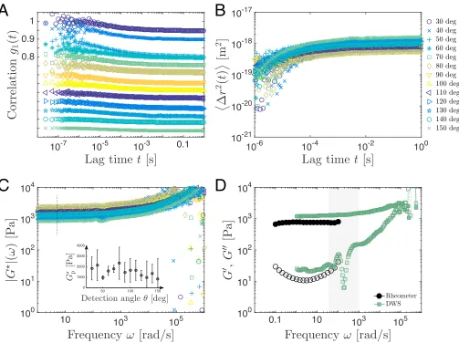
FIG. 5: Measurements on a solid-like, non-ergodic sample, an aqueous gelatin gel at a concentration of 5 wt% with embedded tracer particles (1.25 wt%,a= 1µm ). (A): Pusey-averaged field autocorrelation functionsg1(t) as a function of lag timet,
measured for detection angles ranging fromθ= 30 deg toθ= 150 deg. Curves are offset vertically by increments of -0.05 for clarity. (B): Mean-square displacements extracted from the same data, plotted as a function of time, yielding fair agreement between measurements taken at different angles. Note that sub-nanometer displacements are accessed. (C)Magnitudes of the corresponding complex shear moduli|G⋆(ω)|as a function of frequencyω. The inset shows plateau valuesG⋆
p, accessed at a
frequency of 5 rad/s (indicated as a dotted line in the main plot), as a function of detection angle. Within the estimated error bars, no strong trend in the data is observed; averaging over data from differentθthus appears justified. (D)Storage modulus
G′(ω) (solid squares) and loss modulus G′′(ω) (open squares) averaged over all measurements taken at different angles as a function of frequencyω. Comparing these averaged moduli to results from conventional oscillatory rheology, withG′(ω) shown as solid black circles andG′′(ω) shown as open black circles, we observe very good agreement.
the viscoelastic response of the sample we obtain an aver-aged viscoelastic response, shown in Fig. 5(D), where we plot the storage modulusG′ (solid squares) and the loss
modulusG′′(open squares) as a function of frequencyω.
The oscillations observed in the data at a frequency of
≈50−200 Hz are likely the result of a mechanical dis-turbance or vibration that we could not eliminate in our experimental light scattering setup on this highly out-of-equilibrium sample. The effect can be directly observed in the measured correlation functions at the correspond-ing time scales, as seen in Fig.5(A). For mechanically weaker samples we have not observed these types of os-cillations in our setup. As a result of the importance
of the time-derivative of
∆r2(t)
in determining the vis-coelastic moduli, the oscillations in theg1(t)-data are
am-plified in the corresponding viscoelastic moduli. The fre-quency range where we do not trust the data as a result of these oscillations is indicated with a grey background in Fig.5(D). Nevertheless, besides these oscillations, we ob-tain very good agreement with measurements performed using a conventional oscillatory rheometer, shown in the same figure as solid black circles for G′ and open black
IV. CONCLUSIONS
We have developed a simple method for properly inter-preting dynamic light scattering data from highly mul-tiple scattering samples using a standard dynamic light scattering setup with a cylindrical sample geometry. By performing ideal random walk simulations within a cylin-drical geometry, we predict the path length distribution
P(s) of photons passing through the sample cell. This en-ables us to extend the use of DWS measurements to stan-dard dynamic light scattering instruments. The method can be applied in the context of microrheology, where the dynamics of embedded tracer particles are used to access the frequency-dependent viscoelastic response of soft materials.
The main strength of our approach, besides not re-quiring a dedicated instrument, lies in the fact that by varying the detection angle we can access a wide range of different effective sample geometries with different av-erage path lengths, using one single cylindrical sample cell. This variation of the detection angle is analogous to performing a series of conventional DWS measurements using a series of sample cells with varying thickness or
with varying tracer particle concentrations.
We have further illustrated the usefulness of our method for DWS-based microrheology on a soft solid, gelatin, for which we obtain a very good agreement with macroscopic oscillatory rheology experiments. Moreover, data recorded for different detection angles enable an im-portant consistency check for the microrheology measure-ments and our results illustrate that the accuracy of such microrheology measurements can be improved by aver-aging over measurements obtained at different detection angles.
Acknowledgments
JM and HMW thank the Royal Society for travel sup-port. The work of FA and HMW forms part of the re-search programme of the Dutch Polymer Institute (DPI), project #738. We thank the Institute for Complex Molecular Systems (ICMS) at Eindhoven University of Technology for support.
Supplementary Information for article ”Diffusing-Wave Spectroscopy in a Standard Dynamic Light Scattering Setup”
Error analysis for DWS and microrheology data
In the following we provide a brief analysis aimed at estimating the relative experimental errors associated with our DWS-based microrheology measurements.
In DWS, the dynamics of tracer particles is quantified in terms of temporal autocorrelation functions, from which the time-dependent mean-square displacement (
∆r2(t)
, hereafter abbreviated as MSD(t) ) of the particles can be calculated. Using a generalized Stokes-Einstein relation, the MSD’s are then converted to viscoelastic moduli, with the magnitude of the complex modulus|G⋆(ω)|approximately proportional to the inverse of the mean-square
displacement at a time scalet= 1/ω.
The relative error in the modulus, ∆G⋆/G⋆, is therefore in good approximation the same as the relative error in
the mean-square displacement ∆MSD/MSD. We identify two main sources of error that ultimately determine this relative error in the measured mechanical response:
1. Statistical errors in the intensity correlation function as a result of the finite measurement duration.
2. For nonergodic samples, additional errors are introduced via the Pusey averaging procedure used to estimate ensemble-averaged temporal autocorrelation functions. These errors are introduced via the relative error in the intensity ratio Y = It
Ie between the time-averaged and the ensemble-averaged scattering intensities.
a. Statistical errors in the intensity correlation function
Given a measurement durationT, the statistical error in the intensity correlation functiong2(t) at lag time t can
be expressed as [31]
∆g2(t)≈6 r
t
T. (9)
Given the Siegert relationg1(t) = p
∆g1(t)≈
3
g1(t) r
t
T. (10)
For the purposes of this error analysis, we assume a simplified relationship between the field correlation function
g1(t) and the mean-square displacement MSD(t),g1(t)≈e−k 2 0/3
˜
s
l⋆MSD(t), withk0the wave vector of the laser light, ˜s
the average path length of photons, andl⋆ the transport mean free path.
We can then express the mean square displacement as MSD(t)≈3l⋆ln(g
1(t)/ k02s˜. With∂MSD/∂g1≈ 3l ⋆
k02˜s 1
g1 ≈
MSD/(g1ln(g1)) and ∆g1≈ g31
q
t
T we can now express the total relative error in the complex modulus as
∆G⋆/G⋆≈∆MSD/MSD≈ MSD1 ∂MSD∂g
1
∆g1≈
1
g1ln(g1)
3
g1 r
t
T (11)
b. Errors introduced during the Pusey averaging procedure
For nonergodic samples, additional errors are introduced via the Pusey averaging procedure used to estimate ensemble-averaged temporal autocorrelation functions. These errors are introduced via the relative error in the intensity ratio Y = It
Ie between the time-averaged and the ensemble-averaged scattering intensities. The resulting
error in the mean square displacement is
∆MSD≈ ∂MSD ∂g1
∂g1
∂Y ∆Y , (12)
where ∂MSD
∂g1 ≈ MSD
g1ln(g1), as derived above.
To arrive at an expression for the second term in Eq.12, we write down the relationship between the field correlation functiong1(t) and the intensity ratioY as explained in the main manuscript,
g1(t) = Y −1
Y +
1
Y
˜
g2(t)−σ2 1 2
, (13)
where ˜g2(t) = 1 + g2(tβ)−1 is the time-averaged intensity autocorrelation function normalized by the coherence factor
β, and σ2 = ˜g
2(t)1 characterizes the short-time intercept of ˜g2(t). This yields the second term in Eq.12 as ∂g∂Y1 ≈ 1
Y2
h
1−p
˜
g2−σ2 i
, and withp
˜
g2−σ2≈1 +Y g1−Y, this results in
∂g1
∂Y ≈
1−g1
Y (14)
The total relative error introduced by the intensity ratioY is thus
∆MSD≈ 1−g1 g1ln(g1)·
∆Y
Y . (15)
Plotting the function f(x) = x1ln(−xx), we observe |f(x)| ≈ 1 for values of xclose to 1. For our solid-like samples,
g1 is close to 1 at long times, and thus
1−g1
g1ln(g1)
≈1; therefore in this case we can make the simple approximation ∆MSD
MSD ≈
∆Y Y .
c. Total estimated error
The total estimated error as a result of the above two main sources of error can then be written as ∆G⋆/G⋆≈∆MSD/MSD≈g 3
12ln(g1) r
t T +
1−g1
g1ln(g1)·
∆Y
Of these two contributions to the experimental error, the latter usually dominates, provided that the measurement duration is sufficiently long, such that the factorqTt becomes small enough. Nevertheless, forg1(t) sufficiently close
to 1, the term ln(1g1) would become very large, and eventually lead to the first term becoming dominant.
Indeed, we expect the errors to be highest for cases whereg1(t) is very close to zero (as a result of the factor g12ln(3 g 1)
or g11ln(−gg11), respectively), or very close to unity (as a result of the factor 1 ln(g1)).
1. Code for data analysis of DWS in a cylindrical cell
a. Full codes (written in Matlab) for analyzing DWS data in a cylindrical cell
The complete numerical codes used for analyzing dynamic light scattering data using the approach outlined in the manuscript can be obtained on the author’s website <www.mate.tue.nl/∼wyss>or on request by sending an email to Hans Wyss at [email protected]. Please also address any questions regarding the code and/or data analysis to the same email address.
The specific code for the random walk simulation for calculating the path length distributionP(s) is listed below.
b. Code for calculating the path length distributions
The main code for calculating the path length distributionP(s) is a simple random walk simulation with step length
l⋆, as described in the main manuscript. Below is the C-code (and the MEX function called by our main Matlab
code) that accomplishes this task; the results are kept track of in the output arrayy, which for each bin corresponding to a segment of detection angle and a segment of path length keeps track of the number of photons exiting the cell within the corresponding angle range and within the corresponding path length range. Angular bins evenly divide the angular space between 0 and 180 degrees; we usually choose 180 bins of 1 degree width. Path length bins are also linearly spaced, with 300 bins total and the 100th bin corresponding to a path length of (L(θ)/l⋆)2
in units ofl⋆,
where L(θ) is the distance between the entry point and the exit point of the simulated photon, as a function of the detection angleθ.
Listing of “pathlengthsCyl P s.c”:
1#include ”mex . h” 2#include <s t d i o . h>
3#include <s t d l i b . h>
4#include <time . h>
5#include <math . h>
6 7 /∗
8 ∗
9 ∗ Function t h a t c a l c u l a t e s t h e p a t h l e n g t h d i s t r i b u t i o n f o r d i f f u s i o n o f p h o t o n s
10 ∗ t h r o u g h a c y l i n d e r
11 ∗
12 ∗/
13
14 void p a t h l e n g t h s C y l (double y [ ] , double x [ ] , s i z e t mrows , s i z e t n c o l s ) 15 {
16 i n t i i ,m, n , s t e p , a n g l e b i n , Nbins , N i t e r , index1 , index2 , i n d e x 3 ; 17 double xx , yy , zz , dxx , dyy , dzz , l s t a r , LL , pi , d e l t a z , weight , d i s t ; 18
24 // srand ( ( u n s i g n e d ) time ( NULL ) ) ;
25 s r a n d ( rand ( ) ˆ time (NULL) ) ; 26
27 f o r(m=0;m<mrows ;m++)
28 {
29 f o r( n=0;n<n c o l s ; n++)
30 {
31 i n d e x 1 =(m % mrows )+mrows∗n ; 32 y [ i n d e x 1 ] = 0 ;
33
34 }
35 }
36
37 f o r( n=0;n<n c o l s ; n++)
38 {
39 d i s t=s q r t (
(−1−c o s ( p i / Nbins∗n ) )∗(−1−c o s ( p i / Nbins∗n ) )+s i n ( p i / Nbins∗n )∗s i n ( p i / Nbins∗n ) ) ;
40 i n d e x 1=2+mrows∗n ;
41 y [ i n d e x 1 ]= c e i l ( d i s t∗d i s t / l s t a r / l s t a r / 1 0 0 ) ; // w r i t e column 2 : t h e w i d t h o f each b i n ( s e t as one hundreds o f t h e e x p e c t e d a v e r a g e number o f
s c a t t e r i n g e v e n t s . )
42 }
43 44
45 f o r( i i =0; i i<N i t e r ; i i ++)
46 {
47 xx=−1+ l s t a r ; 48 yy =0; z z =0; 49 s t e p =1;
50 while ( ( xx∗xx+yy∗yy )<1)
51 {
52
53 // Random u n i t v e c t o r o f l e n g t h l s t a r :
54 dxx =2; dyy =2; dzz =2;
55 while ( dxx∗dxx+dyy∗dyy+dzz∗dzz>1) // make s u r e ( dxx , dyy , d z z ) i s a v e c t o r o f random d i r e c t i o n .
56 {
57 dxx=2∗(double) ( rand ( ) ) / (double) (RAND MAX)−1; 58 dyy=2∗(double) ( rand ( ) ) / (double) (RAND MAX)−1; 59 dzz =2∗(double) ( rand ( ) ) / (double) (RAND MAX)−1;
60 }
61 LL=s q r t ( dxx∗dxx+dyy∗dyy+dzz∗dzz ) ;
62 dxx=dxx/LL∗l s t a r ; dyy=dyy/LL∗l s t a r ; dzz=dzz /LL∗l s t a r ; 63 // P r o p a ga t e by a s t e p l s t a r :
64 xx=xx+dxx ; yy=yy+dyy ; z z=z z+dzz ;
65 s t e p ++;
66 }
67 LL=s q r t ( xx∗xx+yy∗yy ) ;
68 xx=xx/LL ; yy=yy/LL ; z z=z z /LL ;
69 a n g l e b i n= c e i l ( a c o s ( xx )∗( Nbins−1)/ p i ) ; 70
71 i n d e x 1=mrows∗a n g l e b i n ; 72 d e l t a z=p i /2/ Nbins ;
73 w e i g h t=e r f ( 3∗d e l t a z / l s t a r / s q r t ( s t e p ) ) ; // a c c o u n t f o r p r o b a b i l i t y i n z−d i r e c t i o n t o h i t area around z z =0
76 // Update a v e r a g e number o f s t e p s and c o r r e s p o n d i n g added w e i g h t s :
77 i n d e x 2 =(1 % mrows )+mrows∗a n g l e b i n ; 78 y [ i n d e x 2 ]=y [ i n d e x 2 ]+ s t e p∗w e i g h t ;
79 i n d e x 3=f l o o r ( s t e p /y [ a n g l e b i n∗mrows +2])+3+mrows∗a n g l e b i n ; 80 i f( f l o o r ( s t e p /y [ a n g l e b i n∗mrows +2])+3<mrows )
81 {
82 y [ i n d e x 3 ]=y [ i n d e x 3 ]+ w e i g h t ; // add v a l u e t o b i n
83 }
84
85 }
86
87 f o r( a n g l e b i n =0; a n g l e b i n<Nbins ; a n g l e b i n++) 88
89 {
90 i n d e x 1=mrows∗a n g l e b i n ;
91 i n d e x 2 =(1 % mrows )+mrows∗a n g l e b i n ; 92 i f( y [ i n d e x 1 ]==0)
93 {
94 // m e x P r i n t f (” y [ i n d e x 1 ] i s z e r o . i n d e x 1 :% i y [ i n d e x 1 ] : %f , y [ i n d e x 2 ] : %f\n ” , index1 , y [ i n d e x 1 ] , y [ i n d e x 2 ] ) ;
95 }
96 i f( y [ i n d e x 2 ]>0)
97 {
98 y [ i n d e x 2 ]=y [ i n d e x 2 ] / y [ i n d e x 1 ] ;
99 }
100 }
101 102 }
103 104 105 106 107
108 void mexFunction ( i n t n l h s , mxArray ∗p l h s [ ] , 109 i n t nrhs , const mxArray ∗p r h s [ ] ) 110 {
111 double ∗x ,∗y ; 112 double l s t a r ; 113 i n t Nbins ;
114 s i z e t mrows , n c o l s , mrows out , n c o l s o u t ; 115
116 /∗ Check f o r p r o p e r number o f arguments . ∗/
117 i f( n r h s !=1) {
118 mexErrMsgIdAndTxt ( ”MATLAB: timestwo : invalidNumInputs ” , 119 ”One i n p u t r e q u i r e d . ” ) ;
120 } e l s e i f( n l h s>1) {
121 mexErrMsgIdAndTxt ( ”MATLAB: timestwo : maxlhs ” , 122 ”Too many output arguments . ” ) ;
123 }
124
125 /∗ The i n p u t must be noncomplex d o u b l e s .∗/
126 mrows = mxGetM( p r h s [ 0 ] ) ; 127 n c o l s = mxGetN( p r h s [ 0 ] ) ;
128 i f( ! mxIsDouble ( p r h s [ 0 ] ) | | mxIsComplex ( p r h s [ 0 ] ) ) {
129 mexErrMsgIdAndTxt ( ”MATLAB: timestwo : i n p u t N o t R e a l S c a l a r D o u b l e ” , 130 ” Input must be noncomplex d o u b l e s . ” ) ;
131 }
133 /∗ A s s i g n p o i n t e r f o r t h e i n p u t m a t r i x .∗/
134 x = mxGetPr ( p r h s [ 0 ] ) ; 135 l s t a r=x [ 0 ] ;
136 // x [ 1 ] = f l o o r ( Nbins ) ;
137 Nbins=x [ 1 ] ; 138
139 /∗ C r ea t e m a t r i x f o r t h e r e t u r n argument . ∗/
140
141 mrows out =303;
142 // row 0 : a v e r a g e i n t e n s i t y f o r t h i s a n g l e b i n ;
143 // row 1 : a v e r a g e p a t h l e n g t h f o r t h i s a n g l e b i n .
144 // row 2 : b i n w i d t h f o r t h i s a n g l e b i n .
145 // rows 3−302: p a t h l e n g t h d i s t r i b u t i o n f o r t h i s a n g l e b i n .
146 n c o l s o u t=Nbins ; /∗ one column f o r each a n g l e segment . The columns g i v e a c o u n t e r f o r each ∗/
147 p l h s [ 0 ] = mxCreateDoubleMatrix ( ( mwSize ) mrows out , ( mwSize ) n c o l s o u t , mxREAL) ; 148
149 /∗ A s s i g n p o i n t e r f o r t h e o u t p u t m a t r i x . ∗/
150
151 y = mxGetPr ( p l h s [ 0 ] ) ; 152
153 /∗ C a l l t h e p a t h l e n g t h s s u b r o u t i n e . ∗/
154 p a t h l e n g t h s C y l ( y , x , mrows out , n c o l s o u t ) ; 155 }
pathlengthsCyl P s.c
[1] G. Maret and P. E. Wolf, Z. Phys. B65, 409 (1987).
[2] D. J. Pine, D. A. Weitz, P. M. Chaikin, and E. Herbolzheimer, Physical Review Letters60, 1134 (1988). [3] D. J. Pine, D. A. Weitz, J. X. Zhu, and E. Herbolzheimer, Journal de Physique51, 2101 (1990).
[4] E. ten Grotenhuis, M. Paques, and G. A. van Aken, Journal of Colloid and Interface Science227, 495 (2000). [5] J. L. Harden and V. Viasnoff, Current Opinion in Colloid & Interface Science6, 438 (2001).
[6] S. Cohen-Addad and R. H¨ohler, Physical Review Letters86, 4700 (2001).
[7] T. G. Mason, H. Gang, and D. A. Weitz, Journal of the Optical Society of America14, 139 (1997). [8] D. A. Weitz, D. J. Pine, P. N. Pusey, and R. J. A. Tough, Physical Review Letters63, 1747 (1989). [9] D. A. Weitz, J. X. Zhu, D. J. Durian, H. Gang, and D. J. Pine, Physica ScriptaT49B, 610 (1993). [10] F. Scheffold, Journal of Dispersion Science and Technology23, 591 (2002).
[11] H. M. Wyss, S. Romer, F. Scheffold, P. Schurtenberger, and L. J. Gauckler, Journal of Colloid and Interface Science241, 89 (2001).
[12] T. G. Mason and D. A. Weitz, Physical Review Letters74, 1250 (1995).
[13] T. G. Mason, K. Ganesan, J. H. van Zanten, D. Wirtz, and S. C. Kuo, Physical Review Letters79, 3282 (1997). [14] T. G. Mason, H. Gang, and D. A. Weitz, Journal of Molecular Structure383, 81 (1996).
[15] T. G. Mason, Rheologica Acta39, 371 (2000).
[16] B. R. Dasgupta, S. Y. Tee, J. C. Crocker, and B. J. Frisken, Physical Review E (2002). [17] P. D. Kaplan, M. H. Kao, A. G. Yodh, and D. J. Pine, Applied Optics32, 3828 (1993). [18] V. L, P. A. Lemieux, and D. J. Durian, Applied Optics40, 4179 (2001).
[19] B. J. Berne and R. Pecora, Dynamic Light Scattering, With Applications to Chemistry, Biology, and Physics (Dover Publications, Mineola, New York, 2000).
[20] P. N. Pusey and W. van Megen, Physica A157, 705 (1989).
[21] F. Scheffold, S. E. Skipetrov, S. Romer, and P. Schurtenberger, Physical Review E63(2001). [22] P. Zakharov, F. Cardinaux, and F. Scheffold, Physical Review E73, 011413 (2006).
[23] K. N. Pham, S. U. Egelhaaf, A. Moussaid, and P. N. Pusey, Review of Scientific Instruments75, 2419 (2004).
[24] M. Reufer, A. H. E. Machado, A. Niederquell, K. Bohnenblust, B. M¨uller, A. C. V¨olker, and M. Kuentz, Journal of Pharmaceutical Sciences103, 3902 (2014).
[25] P. N. Pusey, Macromolecular Symposia79, 17 (1994).
[26] J. G. H. Joosten, E. T. F. Gelad´e, and P. N. Pusey, Physical Review A42, 2161 (1990).
[29] L. F. Rojas-Ochoa, S. Romer, F. Scheffold, and P. Schurtenberger, Physical Review E65, 051403 (2002). [30] D. Durian, Physical Review E51, 3350 (1995).