[NORMAL] An isogeometric continuum shell element for non-linear analysis

This is a repository copy of

An isogeometric continuum shell element for non-linear

analysis

.

White Rose Research Online URL for this paper:

http://eprints.whiterose.ac.uk/96204/

Version: Accepted Version

Article:

Hosseini, S., Remmers, J.J.C., Verhoosel, C.V. et al. (1 more author) (2014) An

isogeometric continuum shell element for non-linear analysis. Computer Methods in

Applied Mechanics and Engineering, 271. pp. 1-22. ISSN 0045-7825

https://doi.org/10.1016/j.cma.2013.11.023

Article available under the terms of the CC-BY-NC-ND licence

(https://creativecommons.org/licenses/by-nc-nd/4.0/)

[email protected] https://eprints.whiterose.ac.uk/ Reuse

This article is distributed under the terms of the Creative Commons Attribution-NonCommercial-NoDerivs (CC BY-NC-ND) licence. This licence only allows you to download this work and share it with others as long as you credit the authors, but you can’t change the article in any way or use it commercially. More

information and the full terms of the licence here: https://creativecommons.org/licenses/

Takedown

If you consider content in White Rose Research Online to be in breach of UK law, please notify us by

An isogeometric continuum shell element for non-linear analysis

Saman Hosseinia_{, Joris J. C. Remmers}a_{, Clemens V. Verhoosel}a_{, Ren´e de Borst}b,∗

a_{Eindhoven University of Technology, Department of Mechanical Engineering, PO BOX 513, 5600 MB, Eindhoven, The Netherlands.} b_{University of Glasgow, School of Engineering, Rankine Building, Oakfield Avenue, Glasgow G12 8LT, UK.}

Abstract

An isogeometric continuum shell formulation is proposed in which NURBS basis functions are used to construct the reference surface of the shell. Through-the-thickness behavior is interpolated using a higher-order B-spline which is in contrast to the standard continuum shell (solid-like shell) formulation where a linear Lagrange shape function is typically used in the thickness direction. The present formulation yields a complete isogeometric representation of the continuum shell. The shell element is implemented in a standard finite element code using B´ezier extraction which facilitates numerical integration on the reference surface of the shell. Through-the-thickness integration is done using a connectivity array which determines the support of a B-spline basis function over an element. The formulation has been verified using different linear and geometrically non-linear examples. The ability of the formulation in modelling buckling of static delaminations in composite materials is also demonstrated.

Keywords: Isogeometric analysis, continuum shell element, solid-like shell element, B´ezier extraction, delamination

1. Introduction

Isogeometric analysis (IGA) has recently received much at-tention in the computational mechanics community. The basic idea is to use splines, which are the functions commonly used in computer-aided design (CAD) to describe the geometry, as the basis function for the analysis rather than the traditional La-grange basis functions [1, 2]. Originally, Non-Uniform Ratio-nal B-Splines (NURBS) have been used in isogeometric aRatio-nal- anal-ysis, but their inability to achieve local refinement has driven their gradual replacement by T-splines [3].

A main advantage of isogeometric analysis is that the func-tions used for the representation of the geometry are em-ployed directly for the analysis, thereby by-passing the need for a sometimes elaborate meshing procedure. This important feature allows for a design-through-analysis procedure which yields a significant reduction of the time needed for the prepa-ration of the analysis model [2]. Indeed, the exact parametriza-tion of the geometry can have benefits for the numerical simu-lation of shell structures, which can be very sensitive to imper-fections in the geometry. Moreover, the higher-order continu-ity of the shape functions used in isogeometric analysis allows for a straightforward implementation of shell theories which re-quire_C1 _{continuity such as Kirchhoff-Love models [4, 5]. A}

Reissner-Mindlin shell formulation has been developed by Ben-son et al. [6] using NURBS basis functions. Although_C1

conti-nuity is then no requisite, good results and a high degree of ro-bustness were reported for large deformation problems. In addi-tion, the exact geometry description allows for an exact

compu-∗_{Corresponding author: Ren´e de Borst, University of Glasgow, School of} Engineering, Rankine Building, Oakfield Avenue, Glasgow G12 8LT, UK.

Email address:[email protected](Ren´e de Borst)

tation of the shell director [7]. Recently, the 7-parameter shell model [8] was cast in an isogeometric formulation in Ref. [9].

A further benefit of basis functions that possess a higher de-gree of continuity is that the computation of stresses is vastly improved. In shell analysis this can be particularly important when materially non-linear phenomena such as damage, or de-lamination, which can occur in laminated structures, are in-cluded in the analysis. In the latter case the computation of an accurate three-dimensional stress field becomes mandatory, and solid-like shell elements become an obvious choice [10, 11]. This shell element is characterized by the absence of rotational degrees of freedom, which is convenient when stacking them, yet possesses shell kinematics, and is rather insensitive to shear locking and membrane locking,

Lagrange polynomials [16].

The continuum shell formulation is outlined in Section 2. In Section 3 we review the basic concepts of isogeometric analy-sis. Algorithmic and implementation aspects are discussed in Section 4. Section 5 contains a number of examples which as-sess the performance of the isogeometric continuum shell for-mulation. The numerical simulations demonstrate the ability of the formulation to model the mechanical behavior of composite structures, including buckling of delaminated panels.

2. Continuum shell formulation

In the solid-like shell element proposed by Parisch [10], an internal stretch term is added to obtain a quadratic term in the displacement field in the thickness direction. As a conse-quence, the normal strain varies linearly, which significantly reduces membrane locking. The element has been extended in [11, 16] for use in laminated composites, including interlami-nar delamination. In Ref. [12] we have described an isogeomet-ric solid-like shell element (SLSBEZ) which utilizes NURBS or T-spline basis functions to construct the mid-surface of the shell. Through the thickness behavior was captured by stan-dard linear shape functions as it is in the conventional solid-like shell element. A complete isogeometric continuum shell ele-ment (CSIGA) which is equipped with the B-spline basis func-tions in the thickness direction is presented here.

2.1. Kinematics

Figure 1 shows the undeformed and the deformed configu-rations of a continuum shell element. The reference surface of the shell is denoted by S0. The variablesξandηare the local curvilinear coordinates in the two independent in-plane direc-tions, andζis the local curvilinear coordinate in the thickness direction. The position of a material point within the shell body in the undeformed configuration is written as a function of the three curvilinear coordinates:

X(ξ, η, ζ)=X0(ξ, η)+ζD(ξ, η), 0_≤ζ _≤1 (1)

where X0(ξ, η) is the projection of the point on the reference surface of the shell and D(ξ, η) is the thickness director perpen-dicular to the surface S0at this point.

In any material point, a local reference triad can be estab-lished. The covariant base vectors are then obtained as the par-tial derivatives of the position vectors with respect to the curvi-linear coordinatesΘi _{=[ξ, η, ζ]. First, we define a set of basis}

vectors on the reference surface in the undeformed configura-tion as:

Eα =

∂X0

∂Θα , α=1,2 (2)

so that the shell director can be written as:

E3=D=

E1×E2 ||E1×E2||

t (3)

ζ

η η

ξ

E2

E1

i1

i2

i3

deformed undeformed

S0

ζ

g2

g₃

ξ

x0

x X

X0

u

E3=D g1

Figure 1: Geometry and kinematics of the shell in the unde-formed and in the deunde-formed configurations.

where t is the thickness of the shell. Now, using equation (1), the covariant triad for any point within the shell body is ob-tained as:

Gα=

∂X

∂Θα =Eα+ζD,α , α=1,2

G3=D

(4)

where the subscript comma denotes partial differentiation. The position of the material point in the deformed configura-tion x(ξ, η, ζ) is related to X(ξ, η, ζ) via the displacement field u(ξ, η, ζ) as:

x(ξ, η, ζ)=X(ξ, η, ζ)+u(ξ, η, ζ) (5)

The displacement field u can be of any order which is in con-trast to the standard solid-like shell formulation where an in-ternal stretch term is added to obtain a quadratic term in the displacement field in the thickness direction. Similarly, in the deformed configuration we can establish the covariant triad as:

gi= ∂x

∂Θi =Gi+u,i , i=1,2,3 (6)

which convention will be used in the remainder. Using equa-tions (4) and (6) the metric tensors G and g can be determined as:

Gi j=Gi·Gj , gi j=gi·gj , i,j=1,2,3 (7)

The contravariant basis vectors needed for the calculation of the strains can be derived as:

Gi=(G)−1Gi (8)

where (G)−1_{is the inverse of the metric tensor with components}

Gi j. The volume of the element in the undeformed

configura-tion is evaluated using the covariant metric tensor G in the fol-lowing manner:

dΩ0= p

det(G) dξdηdζ (9)

2.2. Strain measure

The Green-Lagrange strain tensorγis defined conventionally in terms of deformation gradient F:

γ=1

2(F

T

·F₋I) (10)

where I is the unit tensor. The deformation gradient can be written in terms of the base vectors as:

F=g_i⊗Gi (11)

which leads to following representation of the Green-Lagrange strain tensor:

γ=γi jGi⊗Gj with γi j=

1

2(gi j−Gi j) (12)

where the summation convention has been used for repeated indices. Substituting equations (4) and (6) for Gi j and gi j into

this relation yields:

γi j=

1

2(Gi·u,j+u,i·Gj+u,i·u,j) (13)

2.3. Material law

In continuum shell elements the stresses are computed us-ing a three-dimensional constitutive relation. Assumus-ing small strains, a linear relation between the rates of the Second Piola-Kirchhoffstress tensor S and the Green-Lagrange strain tensor can be adopted:

DS=C_{:Dγ (14)}

whereC_{is the material tangential stiffness matrix.}

The strain field in equation (13) is defined in the parametric frame of Gi,i=1,2,3, which are not necessarily orthonormal. In order to obtain the strains in the element local frame of ref-erence Ti, they must be transformed using:

γL_{i j}=γkltkitl j , tki=Gk·Ti (15)

For an orthotropic material, T1 is the fiber direction. T2 and T3are the in-plane and out-of-plane normal directions, respec-tively.

2.4. Virtual work and linearization

In a Total Lagrangian formulation the internal virtual work is expressed in the reference configurationΩ0:

δWint= Z

Ω0

δγT : S dΩ0 (16)

The resulting system of non-linear equations is typically solved in an incremental-iterative manner, which requires computation of the tangential stiffness matrix. This quantity is obtained by linearizing the internal virtual work, equation (16):

D(δWint)= Z

Ω0

(δγT:_DS + _D(δγT) : S)dΩ0 (17)

withδγand_D(δγ) defined as:

δγi j =

1

2(gi·δu,j+δu,i·gj) (18) and

D(δγi j)=

1

2(D(u,i)·δu,j+δu,i· D(u,j)) (19) In an incremental iterative solution scheme, the strain incre-ment∆γwith respect to the previous converged solution is nor-mally needed. Using equations (13) and (6), it can be derived as:

∆γi j=γi j(u+ ∆u)−γi j(u)

= 1

2(gi·∆u,j+ ∆u,i·gj+ ∆u,i·∆u,j) (20)

3. Isogeometric finite element discretization

In this section we review some basic concepts of isogeomet-ric analysis. Next, the B´ezier extraction technique will be out-lined. This technique is utilized to make a finite element data structure for the spline basis functions.

3.1. Fundamentals of NURBS and B-splines

A B-spline is a piecewise polynomial curve composed of a linear combination of B-spline basis functions:

C(ξ)= n X

i=1

Ni,p(ξ)Pi (21)

where p is the order and n is the number of the basis functions. The Ni,p(ξ) represents a B-spline basis function and the coeffi

-cients Pi are points in space, referred to as control points.

B-splines are defined over a knot vector,ΞΞΞ, which is a set of non-decreasing real numbers representing coordinates in the param-eter domain:

Ξ

ΞΞ =[ξ1, ξ2, ..., ξn+p+1] (22)

Parametric coordinatesξidivide the B-spline into sections. The

positive interval [ξ1, ξn+p+1] is called an element. If all knots are

equally spaced, the knot vector is called uniform, or if they are unequally spaced, they are non-uniform. Between two distinct knots (knot span), a B-spline basis function has_C∞_continuity

while it reduces to_Cp−1_{across a knot. If a knot value appears}

k times, the knot is called a multiple knot. At this knot the continuity is_Cp−k_{. A B-spline is said to be open if its first and}

last knots appear p+1 times.

In one dimension, B-spline basis functions are defined using the Cox-de Boor formulation [17, 18] starting with piecewise constants (p=0):

Ni,0(ξ)=       

1 ξi≤ξ < ξi+1

0 otherwise (23)

from which the higher-order functions p_≥1 are derived recur-sively using:

Ni,p(ξ)= ξ₋ξi ξi+p−ξi

Ni,p₋1(ξ)+

ξi+p+1−ξ

ξi+p+1−ξi+1

ξ Ni,3

0 1

4

1 2

3

4 1.0

0 1

Figure 2: Third-order B-spline basis functions defined over a knot vectorΞΞΞ =[0,0,0,0,1₄,1₂,3₄,1,1,1,1].

Figure 2 shows the B-spline basis functions Ni,3, defined over

the knot vectorΞΞΞ = [0,0,0,0,1₄,1₂,3₄,1,1,1,1]. Using tensor products, B-spline surfaces can be constructed using two knot vectorsΞΞΞ = _{ξ1, ξ2, ..., ξn+p+1}, H = {η1, η2, ..., ηm+q+1}and a

set of n_×m control points Pi,jknown as the control net. By

defining univariate basis function Ni,p and Mj,pover these two

knot vectors, the B-spline surface is then constructed as

S (ξ, η)= n X

i=1 m X

j=1

Ni,p(ξ)Mj,q(η)Pi,j (25)

B-spline basis functions satisfy the partition of unity prop-erty. Also each Ni,p has a local support which is contained in

the interval [ξi, ξi+p+1]. Generally, open B-splines are used in

numerical analysis, since they are interpolatory at the bound-ary, which facilitates the application of Dirichlet boundary con-ditions.

A drawback of B-splines is their inability to represent engi-neering objects such as conical sections exactly. For this reason, Non-Uniform Rational B-Splines (NURBS), which encapsulate B-splines and can represent such objects exactly, have become the standard in Computer Aided Design (CAD). NURBS are defined by augmenting each control point with a weight Wi>0

as Pi=(xi,yi,zi,Wi). Such a point can be represented with

ho-mogeneous coordinates Pw_i =(Wixi,Wiyi,Wizi,Wi) in a

projec-tiveR4_{space. Accordingly, NURBS basis functions are defined}

as:

Rα,p=

Nα,p(ξ)Wα

W(ξ) (26)

where_W(ξ)=Pn

i=1Ni,p(ξ)Wiis the weighting function. Note

that there is no summation implied over the repeated indexα, and that a B-spline is recovered when all the weights are equal. The NURBS surfaces are constructed by the weighted tensor product of B-spline functions, similar as done for B-spline sur-faces, see equation (25).

3.2. B´ezier extraction

As noted in the previous section the parametric coordinates ξiin a knot vector divide the parameter domain into elements.

Similar to the finite element method, these elements, which re-fer to the knot intervals _{ξi, ξi+1}with a positive length, allow

for piecewise integration using quadrature rules. Basis func-tions Ni,p have a local support over a knot interval{ξi, ξi+p+1},

which means that each element supports different basis func-tions, see Figure 3. This is at variance with the finite element method where numerical integration is done on a single parent element. In order to blend isogeometric analysis into existing finite element computer programs, B´ezier elements and B´ezier extraction operators are used to provide a finite element struc-ture for B-splines, NURBS [19], and T-splines [20].

0 1

˜ ξ Ni,3

0

-1 1

˜ ξ 0

-1 1

˜ ξ 0

-1 1

˜ ξ 0

-1 1

Figure 3: B-spline basis functions plotted over [₋1,1]. The basis functions are different per element which is in contrast with standard finite elements.

In general, a degree p B´ezier curve is defined by a linear combination of p+1 Bernstein basis functions B(ξ) [21]. Sim-ilar to B-splines, by having an appropriate set of control points, a B´ezier curve is written as C(ξ) = PTB. A B´ezier extrac-tion operator maps a piecewise Bernstein polynomials basis onto a B-spline basis. This transformation makes it possible to use B´ezier elements as the finite element representation of B-splines, NURBS, or T-splines.

The extraction operator can be obtained by means of knot insertion. Consider a knot vectorΞΞΞand a set of control points

{Pk}n_k=1. By inserting a knot value ¯ξin the knot vector, a new

set of control points needs to be calculated. This new set can be related to the initial set of control points via:

¯

P=[C1]TP (27)

This relation ensures that the parametrization is not changed when an existing knot value is repeated, see [19, 21] for algo-rithms to determine the operator C1. The knot insertion pro-cess is repeated until all interior knots of the knot vector have a multiplicity equal to p, with p the order of the original spline defined over the knot vectorΞΞΞ. Next, the complete set of new control points_{P¯k}m_k=1, with m=nep+1 and nethe number of

elements, is obtained as:

¯

P=[CN¯−N]T[CN¯−N−1]T_{· · ·}[C2]T[C1]TP=CTP (28) Again, the parametrization remains unchanged upon the inser-tion of the addiinser-tional knots. Hence, according to equainser-tion (21) and using equation (28) it is expressed as:

C(ξ)=PTN(ξ)=P¯TB(ξ)=(CTP)TB(ξ) (29)

Since P is arbitrary, the refined basis functions B are related to the original basis functions N via:

N(ξ)=CB(ξ) (30)

Hence, every original basis function can be expressed as a lin-ear combination of the Bernstein polynomials. By defining the operators Leand ¯Leto select the basis functions Neand Befor

element e, we have:

Ne=LeN , B=L¯eBe (31)

Combining equations (30) and (31) leads to

Ne=LeC ¯LeBe (32)

The element extraction operator Ceis defined as:

Ne=CeBe (33)

which, using equation (32) can be elaborated as:

Ce=LeC ¯Le (34)

As can be observed from Figure 4, the B´ezier extraction oper-ator of an element Cemaps a piecewise Bernstein polynomial

basis onto a B-spline basis.

0 1

˜ ξ Bi

0

-1 1

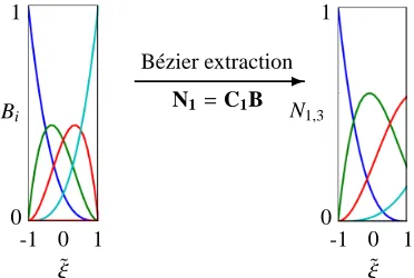
B´ezier extraction

✲ N1=C1B

0 1

˜ ξ N1,3

0

-1 1

Figure 4: Schematic representation of the B´ezier extraction op-erator.

The B´ezier extraction operator for multivatriate B-splines and NURBS can be computed by exploiting their tensor prod-uct strprod-ucture, see [19] for details. For a detailed discussion of B´ezier extraction for T-splines, for which a global tensor prod-uct strprod-ucture is absent, see [20]. From the element extraction operator, B´ezier elements and the global B´ezier mesh can be constructed.

3.3. Isogeometric finite element implementation

Similar to the previous work on the isogeometric solid-like shell element [12], we start by modelling a reference surface S0 _{of the shell, where in this case S}0_{is the bottom surface of}

the shell, see Figure 1. Accordingly, the three-dimensional rep-resentation of the shell reduces to a bivariate description using B´ezier elements, where the geometric and the kinematic quan-tities are approximated by NURBS functions. B´ezier elements for the surface of the shell in combination with linear shape

functions in the thickness direction can fully describe the shell geometry in the undeformed configuration as in equation (1). Therefore, any material point in the shell is obtained as a sum-mation of its projected position vector onto the reference sur-face, X0 _{and its parametric thickness times the shell director,}

ζD.

We assume a higher-order interpolation of the displacement in the thickness direction by using B-spline basis functions. By using equation (24) for example, quadratic B-spline basis func-tions can be defined over a knot vector T =[0,0,0,1₂,1,1,1]. Figure 5 shows the resulting basis functions.

ζ Hi

0 0.5 1.0

0 1

Figure 5: A quadratic B-spline basis function to be used for through the thickness discretization in the deformed configura-tion. The order of the basis_{Hi}4_i=1can be chosen arbitrarily.

The total displacement field is now discretized as:

u(ξ, η, ζ)= ncp

X

I=1

NI(ξ, η, ζ)aI (35)

where aI are the displacement degrees of freedom. We assume

that n and m are the number of shape functions (or the control points) in the reference surface and in the thickness direction, respectively (ncp=n×m). Hence, the shape functions NI read:

NI(ξ, η, ζ)=Si(ξ, η)Hj(ζ),

I=i+( j₋1)n,

i_{∈ {}1, ...,n_} , j_{∈ {}1, ...,m_}.

(36)

where Si(ξ, η) is the basis function from the B´ezier element and Hj(ζ) is the B-spline function in the thickness direction. This

equation implies that the trivariate basis functions NI are

de-composed into a surface part and a thickness part which can have different orders of interpolation, ps and ph, respectively.

As will be detailed below, the strains are subsequently com-puted from these displacements using shell kinematics.

As we only model a surface of the shell rather than the com-plete geometry, it is assumed that every control point on the reference surface has 3_×m degrees of freedom, where m is the number of control points in the thickness direction. Therefore, in a B´ezier mesh each control point Picontains a vector of

de-grees of freedom_Φi, as follows:

Φi=[a1x,a 1 y,a

1 z, ...,a

m x,a

m y,a

m z]

where ax,ay,az denote the displacement components.

Further-more, by combining equations (35) and (36) the displacement components can be written as follows:

uk(ξ, η, ζ)= m X

j=1 n X

i=1

a_kjiSi(ξ, η)Hj(ζ) (38)

where the subscript k refers to the 1, 2, 3 (or x,y,z) directions.

3.4. Evaluation of internal force vectors and stiffness matrices

For the evaluation of the tangential stiffness matrices we first define the virtual strain vector:

δγT =[δγ11, δγ22, δγ33,2δγ12,2δγ23,2δγ31] (39)

This vector is related to the control points degrees of freedom as:

δγ=Bδ_Φ (40)

Referring to equation (18) this equation is expanded as:

δγ=[B1B2_{· · ·}Bm]6×3ncp·[Φ

1

Φ2· · ·Φm]T_3n

cp (41)

where

[Bj]6_×3n·[Φj]T3n=[b j1

bj2_{· · ·}bjn]_·[φj1φj2_{· · ·}φjn]T (42)

In this equation, bjia 6_×3 matrix with the components:

b_1kji =g1·ikSi,ξHj

b_2kji =g2·ikSi,ηHj

b_3kji =g3·ikSiHj,ζ

b_4kji =g1·ikSi,ηHj+g2·ikSi,ξHj

b_5kji =g2·ikSiHj,ζ+g3·ikSi,ηHj

b_6kji =g1·ikSiHj,ζ+g3·ikSi,ξHj

(43)

where ik,k=1,2,3 are the unit base vectors of the global

co-ordinate system, and

φT_ji=[axjia ji ya

ji

z] (44)

with a_kji used in equation (38). As an example we will de-rive the explicit expression for the virtual strain componentγ11

in Appendix A. It is emphasized that the virtual strains and the corresponding B matrix in equation (40) are stated in the non-orthonormal curvilinear base vectors which should be trans-formed to the element local frame according to equation (15). The transformed B matrix is represented by BL, which is given

in Appendix B.

From the internal virtual work, equation (16), the internal force vector is directly obtained as:

fint= Z

Ω0

BT_LS dΩ0 (45)

Next, we rewrite the linearized internal virtual work, equa-tion (17), in matrix form:

−D(δWint)=δΦT

∂fint

∂_ΦDΦ=δΦ T_K

DΦ

=δ_ΦT(Kmat+Kgeom)_DΦ

(46)

where K represents the stiffness matrix decomposed in a ma-terial part Kmat_{and a geometric part, K}geom_{, as usual. From}

equation (17) these matrices can be obtained as:

Kmat= Z

Ω0

BT_LCBLdΩ0 , Kgeom= Z

Ω0 ∂BT_L

∂_ΦS dΩ0 (47)

The geometric part is the stress-dependent part of the stiffness matrix and is obtained through the derivatives of the virtual strains, equation (19). Using the notation:

ωkl=tkitl jSi j (48)

with Si j the components of the Second Piola-Kirchhoffstress

tensor and tkidefined in equation (15), the integrand of the

ge-ometrical part of the stiffness matrix can be written as:

∂BT_L ∂_Φ =Λ

T

Λ (49)

where

ΛT =[λ1,λ2,_{· · ·},λm]3ncp×3 (50) with

λj=[λj1,λj2,_{· · ·},λjn]T_3n×3 (51) and

λji=_S

i,ξHj√ω11+Si,ηHj√ω22+SiHj,ζ√ω33 + Si,ξHj+Si,ηHj√ω12

+ Si,ηHj+SiHj,ζ√ω23

+ Si,ξHj+SiHj,ζ√ω13I (52)

Herein, i refers to layer i and I is the 3_×3 unit matrix.

4. Numerical aspects

The linearized internal virtual work relation derived in equa-tion (17) is discretized using B-spline basis funcequa-tions. A dis-tinction is made between the discretization of the in-plane and the out-of-plane displacement fields. Regarding the latter, we will derive three variants. In the first variant, all layers of the shell element are represented by a single higher-order B-spline in the thickness direction. In the second variant, interfaces be-tween layers are represented by weak discontinuities. In the third version of the element a static delamination is modelled by introducing a strong discontinuity in the B-spline function.

4.1. In-surface and out-of-surface integration

As mentioned in the formulation of B-splines and NURBS, the basis functions are defined over a parametric knot span, i.e (ξ, η, ζ)_∈[0,1]3_{. In order to carry out the numerical integration}

the basis functions and their derivatives should be calculated locally at quadrature points defined over a parent element, i.e ( ˜ξ,η,˜ ζ˜) _∈ [₋1,1]3. Moreover the corresponding Jacobian de-terminant of the mapping must be calculated. The mapping for all the parametric coordinates is the same. For example, for a thickness element of [ζk, ζk+1] the mapping is (Figure 6):

ζ=ζk+( ˜ζ+1)

ζk+1−ζk

2 (53)

where ˜ζ is the parent element coordinate. Therefore the kine-matic parameters in terms of B-spline and NURBS parametric coordinate should be written in the right format. For instance, equation (4) is rewritten as:

Gα =

∂X

∂Θα˜ =Eα˜ +

ζk+( ˜ζ+1)

ζk+1−ζk

2

D,α˜ , α˜ =1,2

G3 =

∂X

∂ζ˜ =

ζk+1−ζk

2 D

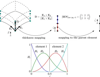
(54) As we employ independent discretizations for the reference surface of the shell and for the thickness direction, the numeri-cal integration schemes in the in-plane and out-of-plane direc-tions will also be decoupled. Accordingly, the B´ezier extraction operator will be used for the integration over the surface. First, the geometry of the reference surface is mapped to its corre-sponding NURBS parametric space (ξ, η) _∈ [0,1]2_{, see}

Fig-ure 7. Then, the second mapping is carried out to the B´ezier space where the parent element ( ˜ξ,η˜)_∈[₋1,1]2_{and the}

extrac-tion operator are obtained.

Through the thickness integration is done by using the con-nectivity array (or IEN array). Using this array we determine which functions have a support in a given element. Assume that we use a quadratic B-spline defined over a knot vector of

T =[0,0,0,1₂,1,1,1], see also Figure 6. This definition leads to two elements of [0,1

2] and [ 1

2,1] over the thickness and four

global basis functions. Each element support ph+1 =3 basis

of the global basis. The IEN array is:

[IEN]ne×ph+1=

1 2 3 2 3 4

!

2_×3

(55)

The assembly of the element stiffness matrices can also be done according to the shared basis functions (number 2 and 3 in this case). It starts from the strain-displacement matrix B:

[B]=

B1e1, B

2 e1+B

2 e2, B

3 e1+B

3 e2, B

4 e2

(56)

which is subsequently used in the calculation of the material part of the stiffness matrix Kmat in equation (47). The same steps are followed for the matrix_Λin equation (50) for the cal-culation of the geometrical part of the stiffness matrix Kgeom.

4.2. Modelling weak and strong discontinuities in the displace-ment field

As has been mentioned in Section 3.1, B-spline and NURBS basis functions are_Cp−k continuous at a knot with multiplic-ity k. This means that we are able to control the continumultiplic-ity of the basis functions at a knot by arbitrarily selecting the multi-plicity. This property is useful in modelling traction-free cracks and adhesive interfaces (strong discontinuity) and layered struc-tures with_C0_{continuity between the layers (weak}

discontinu-ity) [13].

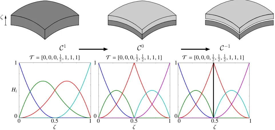
Figure 8 shows the steps in order to make a discontinuity in the thickness direction of a shell structure. Assume that a quadratic B-spline basis function Hi defined over a knot

vec-tor_T = [0,0,0,1₂,1,1,1] has been used in the thickness of the shell. This gives us four basis functions which are all_C1

continuous at ζ = 1₂. Now suppose that we want to have a composite shell consisting of two layers of equal thickness. The deformation of composite structures requires a unique dis-placement at the interfaces and different strain fields in the adjacent layers. In the example of Figure 8 this is simply achieved by having a displacement field which is_C0 continu-ous at the interfaceζ = 1₂. This leads to the new knot vector

T = [0,0,0,₂1,1₂,1,1,1]. Henceforth, we will denote this el-ement as the layered CSIGA elel-ement. Subsequently, the com-plete separation of the layers is obtained if we insert the second knot as: _T =[0,0,0,1₂,1₂,1₂,1,1,1], and this element will be denoted as the discontinuous CSIGA element. Figure 8 shows the corresponding basis functions through the knot insertion process.

It is important to note that if this method to introduce weak or strong discontinuities is adopted in the construction of a single volumetric B-spline or NURBS patch, the inserted discontinu-ity will have a global influence, i.e. it will propagate throughout the patch. While this is not a problem for when weak discon-tinuities are inserted to model layers, it can be restrictive when used to model delamination by means of strong discontinuities. In Section 5.6 we will demonstrate how linear constraints can be used to localize strong discontinuities in order to realisti-cally mimic delaminations. In a further study we will develop a versatile method to localize strong discontintuities. This can potentially be achieved by adopting a localized definition of the basis functions – as is essentially done in T-splines – and has already been demonstrated in the context of cohesive-zone modelling [13].

5. Numerical simulations

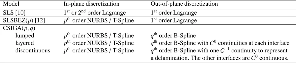
The isogeometric continuum shell formulation is now veri-fied and assessed through different examples. We refer to the proposed class of shell elements as CSIGA, see Table 1. In this table we distinguish between three cases for the contin-uum shell element: (i) without _C0 _{planes between the layers}

(lumped), (ii) with_C0_{planes between the layers (layered), and}

(iii) with_C−1_{planes to simulate static delamination}

ζ

Z E2

˜ ζ [IEN]ne×ph+1=

1 2 3 2 3 4

E1

thickness mapping D= E1×E2

||E1×E2|| D

mapping to the parent element

ζ Hi

0 0.5 1

0 1

element 1 element 2

H1 H2 H3 H4

Figure 6: A quadratic B-spline basis function to be used for through the thickness discretization in the deformed configuration. The basis functions are defined over a knot vector of [0,0,0,1

2,1,1,1] which gives two elements over [0, 1 2] and [

1

2,1]. The numerical

integration is done by defining the IEN-array which determines which functions have support in a given element. It should be noted that we do not consider any control point in the thickness direction where the thickness director D can be calculated directly from the in-surface base vectors E1and E2.

as well as in the out-of-plane direction for each case. For in-stance, in the remainder ”lumped(3,2)” will denote a CSIGA element without _C0 _{(weak discontinuity) planes between the}

layers, with a third-order NURBS/T-spline interpolation in the plane, and a second-order B-spline in the thickness direction.

In the beginning we examine the locking problem which is typical for shell elements. We proceed the simulations by a linear calculation on a composite panel, which aims to capture the global and local behavior of the panel (deflection and stress distribution, respectively). Then, the element will be tested us-ing some geometrically non-linear examples of a pinched hemi-sphere and pinched cylinder with inward and outward loads. These simulations are followed by modelling buckling of de-laminated zones in layered panels.

5.1. Locking

In this section we investigate shear locking and membrane locking which can occur when decreasing the thickness of shell elements. A clamped plate and a cylindrical shell, both under bending loads are used to assess the locking phenomenon.

5.1.1. Shear locking

Figure 9 shows the geometry of a plate subject to bend-ing [11]. The plate has a Young’s modulus E = 1.08 _{Pa and}

a Poisson’s ratio ν = 0.3. The dimensions of the plate are: L=10 m, b=1 m and the thickness t varies through the test. The plate is clamped at one end and a transverse load qz=100t3

is applied at the other end.

As a reference value we consider the displacement at the free end according to the beam theory,δ =PL3_{/3EI which results}

inδ=0.004 m for this test. The numerical simulation is done with two meshes of 64 CSIGA lumped(2,2) and 64 CSIGA lumped(3,2) elements. Figure 10 shows the obtained normal-ized displacements for different ratios of L/t. It is clear that employing second order and third order NURBS basis func-tions for the in-plane discretization result in shear locking free behaviour as the thickness of the plate reduces.

5.1.2. Membrane locking

Membrane locking can occur in curved structures [8, 9]. Therefore, a cylindrical shell as shown in Figure 11 is mod-elled. The shell has a radius of R = 10 m and a width of b = 1 m. Young’s modulus and Poission’s ratio are 1000 Pa andν=0 respectively. The cylindrical shell is clamped at one edge and subjected to a constant distributed load of qx=0.1t3.

An analytical solution based on the Bernoulli beam theory gives a value of approximately 0.942 for the radial displacement.

The numerical results for various meshes and thicknesses are presented in Figure 12. In the figure, the mesh size shows the number of elements in the radial direction, while only one ele-ment has been used in the width direction. According to the results, a low number of elements of order two, 16 CSIGA lumped(2,2) elements, exhibit membrane locking. Keeping the NURBS order fixed and increasing the number of elements to 64 removes locking. Employing 16 third-order NURBS ele-ments the results are locking-free as well.

˜

ξ

η

˜

η

ξ

physical element

B´ezier element

B´ezier mapping

parametric NURBS element

X

Y _{the reference surface of the shell,S}0

geometrical mapping of

Figure 7: Numerical integration on the reference surface of the shell is done using the extraction operator. The geometry of the reference surface is mapped to the corresponding NURBS parametric space. A second mapping is made onto the B´ezier space where the extraction operator and the parent element are obtained.

C

C

C

ζ Hi

0

0.5 1

0

1 T

=[0,0,0,1₂,1,1,1]

ζ 0

0.5 1

0

1 T

=[0,0,0,1₂,1₂,1,1,1]

ζ 0

0.5 1

0 1 T

=[0,0,0,1₂,1₂,1₂,1,1,1]

Figure 8: Schematic representation of introducing a discontinuity in the thickness direction of a shell. Weak and strong discontinu-ities between the layers of a composite shell are created by knot insertion.

5.2. Composite laminate

The performance of the shell element is studied in the sim-ulation of the deflection of a multi-layer composite panel. In

Table 1: Nomenclature of solid-like and continuum shell elements.

Model In-plane discretization Out-of-plane discretization SLS [10] 1st_{or 2}nd_{order Lagrange 1}st_{order Lagrange}

SLSBEZ(p) [12] pth_{order NURBS/T-Spline 1}st_{order Lagrange}

CSIGA(p,q)

lumped pth_{order NURBS/T-Spline q}th_{order B-Spline}

layered pth_{order NURBS/T-Spline q}th_{order B-Spline with}

C0_{continuities at each interface}

discontinuous pth_{order NURBS/T-Spline q}th_{order B-Spline with one}

C−1_{continuity to represent}

a delamination. The other interfaces are_C0_continuous.

L b

t

qz

Figure 9: Geometry of the clamped plate under bending.

0.8 0.85 0.9 0.95 1 1.05 1.1 1.15 1.2

0 50 100 150 200 250 300 350 400 64 lumped(2,2)

64 lumped(3,2)

N

o

rm

a

li

z

e

d

d

is

p

la

c

e

m

e

n

t

Ratio length to thickness, L/t

Figure 10: Normalized displacement of the plate under bending obtained for different ratios of L/t.

qx

t b

ux

x

z R

y

Figure 11: Geometry of the cylindrical shell

allow for computing the stresses and strains in the individual layers accurately.

We consider the square laminate shown in Figure 13. The panel has dimensions a_×b = 0.6_×0.4 m and consists of six

0.2 0.3 0.4 0.5 0.6 0.7 0.8 0.9 1 1.1

0 100 200 300 400 500 600 700 16 lumped(2,2)

64 lumped(2,2) 16 lumped(3,2) Bernoulli

R

a

d

ia

l

d

is

p

la

c

e

m

e

n

t,

ux

Slenderness R/t

Figure 12: Cylindrical shell, displacement uxfor different ratios

of R/t.

00 00 11 11

00 00 11 11

000 000 111 111

00 00 11 11

000 111 00001111 00

00 11

11 000

000 111 11100

00 11 11000000111111

000 000 111 111

t

b

a

Figure 13: Geometry, boundary conditions and loading of a rectangular panel.

layers of a unidirectional material, with a stacking sequence [0,90,0]s. Each layer is 0.2 mm thick, so that the total

thick-ness of the shell is 1.2 mm. The layers can be modelled as a transversely isotropic material with E1=130 GPa, E2 =E3 =

7 GPa,ν12 =0.33 and G12 =5 GPa. The panel is simply

sup-ported on all four sides and is loaded by a distributed load

qz=q0sin

πx a sin

πy b

with q0=1 MPa.

The panel has been simulated for three different discretiza-tions: second-order in the thickness direction, fourth-order in the thickness direction, and second-order per layer with weak discontinuities at the boundaries between the layers.

The analytical solution can be obtained from classical lam-inate theory. The deflection of the mid point of the panel is equal to ₋2.62_×10−5_{m. Figure 14 shows σ}

xx in the

mid-point of the panel as a function of the thickness coordinate

of the shell obtained for different discretizations. The results from one second-order and one fourth-order B-spline element, lumped(3,2) and lumped(3,4), respectively, lead to the same stress distribution as that of a second-order B-spline per layer (weak discontinuities at layer boundaries). All the results are in agreement with the analytical solution from the classical lami-nated plate theory. Moreover, the deflection at the mid-point of the panel is in agreement with the analytical solution.

−0.6 −0.4 −0.2 0 0.2 0.4 0.6

−60000 −40000 −20000 0 20000 40000 60000 lumped(3,2)

lumped(3,4) layered(3,2) clpt

T

h

ic

k

n

e

ss

c

o

o

rd

in

a

te

[m

m

]

Stress,σxx[MPa]

Figure 14:σxxat the mid-point as a function of the thickness of

the panel. The thickness of the plate is 1.2 mm.

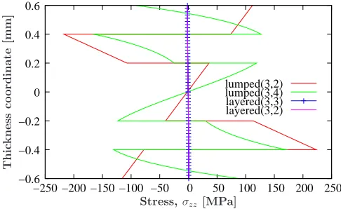
Next, the ability of the shell element to compute interlaminar stresses is examined. This issue is of importance when damage and failure of composite materials need to be considered in the simulations. The normal stressσzzis presented in Figure 15 as

a function of thickness of the shell. By using third-order and second-order B-splines per layer, layered(3,3) and layered(3,2) elements, respectively, which are _C0 _{continuous at the}

inter-faces, we can capture aσzz distribution in the thickness

direc-tion, which is zero through most of the thickness and equals q0 = 1 MPa at the top surface. Adopting just one element of

second-order and of fourth-order B-splines, lumped(3,2) and lumped(3,4), respectively, for the discretization in the thickness direction results in a fluctuation of theσzz distribution. From

the results it is concluded that in order to computeσzz

accu-rately we need to enforce_C0-continuity of the basis functions at the interfaces.

The simulations are now repeated for a ten times thicker panel with q0 =100 MPa. The results presented in Figure 16

show again that applying basis functions with_C0_continuity

be-tween the layers results stress distribution that can be expected for a thick panel. The jump at z =0 is caused by the fact that the displacement boundary condition uz = 0 at the edges has

been enforced at z=0.

5.3. Pinched hemispherical shell with a hole

A pinched hemisphere with a hole at the top has been used extensively as a benchmark problem for shell analysis to test the ability to describe nearly inextensional bending modes [22, 23, 24]. The geometric parameters and material properties employed in this test are summarized in Table 2. The

−0.6 −0.4 −0.2 0 0.2 0.4 0.6

−250 −200 −150 −100 −50 0 50 100 150 200 250 layered(3,2)

layered(3,3) lumped(3,4) lumped(3,2)

T

h

ic

k

n

e

ss

c

o

o

rd

in

a

te

[m

m

]

Stress,σz z[MPa]

Figure 15:σzzat the mid-point as a function of the thickness of

the panel. The thickness of the panel is 1.2 mm (thin panel).

−6 −4 −2 0 2 4 6

−400 −300 −200 −100 0 100 200 300 lumped(3,2)

lumped(3,4) layered(3,3) layered(3,2)

T

h

ic

k

n

e

ss

c

o

o

rd

in

a

te

[m

m

]

Stress,σz z[MPa]

Figure 16:σzzat the mid-point as a function of the thickness of

the panel. The thickness of the panel is 12 mm (thick panel).

shell is subjected to two opposite point loads. The bottom cir-cumferential edge of the hemisphere is free. Due to the sym-metry only a quarter of the shell needs to be modelled. The symmetric boundary conditions are applied by constraining the displacement degrees of freedom in the normal direction of the symmetry plane. The mesh and the applied boundary condi-tions are shown in Figure 17. ABAQUS has been used to gen-erate a standard finite element solution, using a 16_×16 mesh consisting of so-called S4R shell elements, which we will here use as a reference solution.

Table 2: Geometric parameters and material properties for the pinched hemisphere.

Radius R Thickness t Young’s modulus E Poisson’s ratioν 10.0 m 0.04 m 6.825_×107_{Pa 0.3}

Figure 17: The mesh for a quarter model and the boundary con-ditions.

those obtained with the CSIGA and S4R elements.

0 50 100 150 200

0 0.5 1 1.5 2 2.5 3 3.5 CSIGA

SLSBEZ S4R

L

o

a

d

[N

]

Displacement [m]

Figure 18: The load P as a function of the displacement at point A for the pinched hemisphere.

5.4. Pinched cylinder with free ends

The pinched cylinder with free ends shown in Figure 19 is used next to assess the element performance. The cylinder has a length L = 10.35 m, a radius R = 4.935 m, a thickness t =0.094 m, a Young’s modulus E =10500 MPa and a Pois-son’s ratioν=0.3125. The cylinder has free edges at the ends, and it is loaded by two centrally located diametrically opposed point forces, which pull in the outward direction. Due to sym-metry considerations only one-eight of the cylinder needs to be modelled.

The initial response is dominated by the bending stiffness which induces large displacements at relatively low load levels. This changes into a very stiffresponse when the displacement become larger. Finite rotations occur afterwards, thus making the pinched cylinder with free ends a challenging test for ele-ment performance [25, 26, 27].

Figure 20 shows the load-displacement curves of this exam-ple. The results have been obtained with a mesh of 16_×16 CSIGA elements of type lumped(3,2), a mesh of 16_×16 SLS-BEZ elements and a mesh of 16_×8 of S4R elements

imple-Figure 19: Pinched cylinder with free ends

mented in ABAQUS. The magnitude of the load is that for the complete cylinder and the displacement is measured at the point where load is applied. From Figure 20 it can be seen that the results from different elements are very close, however the CSIGA elements show a softer response.

0 5 10 15 20 25 30 35 40

0 0.5 1 1.5 2 2.5 3 CSIGA

S4R SLSBEZ

L

o

a

d

[N

]

Displacement [m]

Figure 20: Load-Displacement diagram of pinched cylinder with free ends.

5.5. Pinched cylinder with rigid diaphragm

The problem of a pinched cylinder with a rigid diaphragm at the ends has been studied by several authors [28, 29, 30] in order to test the convergence behaviour and non-linear perfor-mance of shell elements. Since large rotations occur the prob-lem provides a test for the finite rotation capability of the shell formulation. The cylinder has a length L = 200 mm, a ra-dius R =100 mm, a thickness t =1 mm, a Young’s modulus E =30000 N/mm2and a Poisson’s ratioν=0.3. The cylinder is loaded by two centrally located, diametrically opposed point forces P, which push inwards. Using symmetry only one-eighth of the structure needs to be modelled.

Numerical simulation have been performed using CSIGA, SLSBEZ and S4R elements. Because of the need for mesh re-finement at the free edge T-spline functions have been used for the in-plane discretization for both the CSIGA and SLSBEZ

ements, see Figure 21. The use of T-splines at the left free edge has been discussed in Ref. [12].

Figure 21: Pinched cylinder with rigid diaphragm

The results of the simulations are shown in Figure 22. The magnitude of the load is that for the complete cylinder and the displacement is measured at the point where load is ap-plied. The CSIGA elements integrated with a 4_×4_×2 inte-gration scheme show locking for displacement level higher than 30 mm. Repeating the simulation with a 2_×2_×2 integration scheme improves the results and compares well with those of the SLSBEZ and S4R elements.

0 500 1000 1500 2000 2500 3000

0 10 20 30 40 50 60

L

o

a

d

[N

]

Displacement [mm] CSIGA(4×4×2)

S4R SLSBEZ CSIGA(2×2×2)

Figure 22: Load-Displacement diagram of pinched cylinder with rigid diaphragm.

5.6. Buckling of static delaminations

In the final examples, we will study the possibility to insert a delamination in layered structures by means of introducing a strong discontinuity through the thickness. The panels tested in the examples are partially delaminated over a strip and over a circular region, respectively.

5.6.1. Buckling of plate with initial strip delamination

We consider the panel shown in Figure 23. The panel has unit dimensions and consists of two layers of an isotropic material. The material properties are: E=2_×104_{MPa andν=0.3. The}

top layer has a thickness 0.01 m and the bottom layer 0.09 m.

The top layer is partially delaminated over a width of 0.75 m. This delamination is modelled by a strong discontinuity in the thickness direction.

Y Z

σ_x

X σ_x

initial delamination

W=1 m

L=_{1 m}

h1=0.09 m h2=0.01 m

Figure 23: Geometry of the panel with a strip initial delamina-tion, which is located between the two layers.

We start by defining the through-the-thickness B-spline func-tions over a knot vector of _T = [0,0,0,0.9,0.9,0.9,1,1,1]. This gives two layers in the thickness which are fully delam-inated. The area that is not delaminated can be modelled by applying a linear constraint between the lower layer and the up-per layer. Figure 24 shows the third-order NURBS meshes used for this example. In these meshes the control points are shown in red and blue. Using equation (37) the vector of degrees of freedom_Φifor each control point is written as:

Φi=[a1x,a 1 y,a

1 z, ...,a

6 x,a

6 y,a

6 z]

T _{, i=1,2, ...,n (57)}

The linear constraint is now applied to the red control points as:

a3x=a4x , a3y=a4y , a3z =a4z (58)

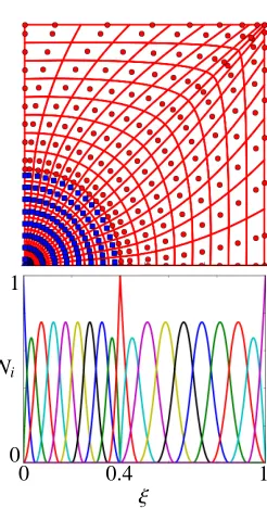
By doing so the degrees of freedom with the superscript 3 and 4 have the same values at the interface of the two layers. It should be noted that the linear constraint is not applied to the blue con-trol points. Referring to the basis functions shown in Figure 24, it can be seen that the basis functions corresponding to the blue control points have a support over the whole delaminated area in the parametric space. Therefore, by excluding their corre-sponding degrees of freedom from the linear constraint space the delaminated area can be preserved.

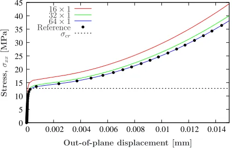
An issue in delamination modelling is the proper selection of the order of the continuity of the NURBS basis functions at the delamination fronts. Figure 25 shows the results obtained with the third-order NURBS basis which are_C2 _{continuous at the}

delamination fronts. The figure presents the out-of-plane dis-placement versus the axial stressσxx for different mesh sizes.

An analytical solution for the buckling stress of a clamped panel with thickness of h=0.01m and length l=0.75m was formu-lated by Kachanov [31]:

σcr= π2_E

3(1₋ν2_{) h}

l

2

=12.84 MPa (59)

✒

❅ ❅ ❅ ■ delamination front

ξ Ni

0

0.5

0.125 0.875 1 0

1

ξ 0

0.5

0.125 0.875 1 0

1

Figure 24: Third-order NURBS meshes used for the panel with initial strip delamination. The left mesh uses _C2 _continuous

basis at the delamination front while in the right mesh_C0

con-tinuous basis functions are used at the delamination front.

0 5 10 15 20 25 30 35 40 45

0 0.002 0.004 0.006 0.008 0.01 0.012 0.014

64×1 Reference

σcr

S

tr

e

ss

,

σx

x

[M

P

a

]

16×1 32×1

Out-of-plane displacement [mm]

Figure 25: Diagram of the axial stressσxxvs the out-of-plane

displacement of the plate with an initial strip delamination. The used meshes are_C2at the delamination fronts.

We repeat the simulation using third-order NURBS basis function, but with a _C0 continuity at the delamination fronts, in order to exactly capture the Dirichlet boundary condition at this position. Figure 26 shows that using 48 NURBS elements the obtained critical stress is in agreement with the reference so-lution of 192 elements and the analytical soso-lution. Accordingly, by applying_C0 _{continuous basis functions at the delamination}

front we can properly capture the boundary condition, which is a basic assumption in the analytical expression for the buckling load. Figure 27 shows a schematic representation of the delami-nation opening resulting from meshes with and without_C0

0 5 10 15 20 25 30 35 40

0 0.002 0.004 0.006 0.008 0.01 0.012 0.014

S

tr

e

ss

,

σx

x

[M

P

a

]

48×1 Reference

σcr

Out-of-plane displacement [mm]

Figure 26: Diagram of the axial stressσxxvs the out-of-plane

displacement of the plate with an initial strip delamination. The used meshes are_C0_{at the delamination fronts.}

tinuity at the delamination fronts. As it can be seen, for the_C0 case the effective length of the initial delamination leis larger

than that resulting from the_C2_{mesh. Referring to the analytical}

solution for the critical buckling stress i.e. equation (59), it is clear that the buckling load is proportional to the inverse of the initial delamination length l. Therefore, for an equal number of elements, a_C0 _{mesh at the delamination front will result in}

a smaller critical buckling stress, which explains the difference between the obtained results. However, the additional effort of enforcing_C0 _{continuity probably does not outweigh the}

com-putational gain, since with 64_C2_{continuous elements the same}

result was obtained. This holds a fortiori when propagating de-lamination fronts are considered.

lC_e0

≈lC2

e

lC0 e >l

C2 e

Figure 27: Schematic representation of the delamination open-ing obtained with meshes which are_C2 _and

C0 _{continuous at}

the delamination front.

5.6.2. Glare panel with a circular delamination

In this section the buckling behavior of a Glare panel with initial circular delamination under uniaxial compressive load is examined. The specimen geometry is shown in Figure 28. The panel consists of an aluminium layer with thickness h1 =

0.2 mm and a Glare 0/90◦ prepreg layer with a thickness 0.3 mm. A circular delamination with radius 8 mm is assumed between the layers. In order to avoid global buckling, a thick layer of aluminum is attached to the panel. Table 3 contains the material parameters of the Glare prepreg.

An advantage of using NURBS basis functions is that we are able to model an exact circular delamination shape.

Y Z

σ_x

Glare, 0.2 mm Al, 0.3 mm

Al, 10 mm

X

W=4 0 mm r=8 m

m

σ_x

initial delamination

L= 40_mm

Figure 28: Geometry of the Glare panel with a circular initial delamination, which is located between the top aluminum layer and the Glare layer.

Table 3: Material parameters for 0/90◦Glare prepreg. E11 =33170 MPa E22 =33170 MPa E33=9400 MPa

G12 =5500 MPa G23 =5500 MPa G13 =5500 MPa

ν12=0.195 ν23=0.032 ν13 =0.032

Similar to the previous example the delamination is mod-elled by a strong discontinuity between the layers where a linear constraint will preserve the adhesion at the remain-der of the panel. In this case we define through the thick-ness B-spline basis functions over a knot vector of _T =

[0,0,0,0.952,0.952,0.971,0.971,0.971,1,1,1]. Accordingly the linear constraint is written as:

a5_x=a6_x, a5_y=a6_y , a5_z =a6_z (60)

Because of the symmetry only one quarter of the geometry is analyzed. Figure 29 shows a second-order NURBS mesh for this example. The basis functions have been chosen to be_C0

continuous at the delamination front. Figure 30 presents the out-of-plane displacement vs the axial stress σxx for two fine

NURBS meshes. Both meshes lead to the same result.

6. Concluding remarks

A continuum shell element has been formulated that is based on the isogeometric concept. NURBS basis functions have been used to parametrize the reference surface, and a B-spline shape function has been employed in the thickness direction. In this manner, a complete three-dimensional representation of the shell is obtained. The shell formulation combines the advan-tages of a full, three-dimensional stress and strain representa-tion that allows for the straightforward implementarepresenta-tion of con-stitutive relations such as plasticity or damage, with the advan-tages of isogeometric analysis, including the exact description of the geometry, the use of the design-through-analysis concept, and the accurate prediction of stress fields. The latter property is also important for the prediction of the onset of plasticity, damage, or delaminations due to high transverse stresses.

In this paper, the performance of the isogeometric continuum shell element has been assessed by means of a number of linear

ξ Ni

0

0.4 1

0 1

Figure 29: The second-order NURBS mesh used for the panel with circular delamination. The basis function are_C0 continu-ous at delamination front.

0 100 200 300 400 500 600

0 0.1 0.2 0.3 0.4 0.5

S

tr

e

ss

,

σx

x

[M

P

a

]

16×16 32×32

Out-of-plane displacement [mm]

Figure 30: Diagram of the axial stressσxxvs the out-of-plane

displacement of the plate with an initial circular delamination.

and non-linear examples. First, the performance with respect to shear and membrane locking was examined for a straight and for a curved clamped strip. The element was found locking-free at least for length to thickness ratios up to 400 provided that cu-bic splines were used for the in-plane discretization or quadratic splines with a sufficiently fine discretization. Next, a unidirec-tional composite panel consisting of six layers of [0,90,0]shas

been tested under a sinusoidal distributed pressure load. It was shown that the global behavior of the panel, deflection and the in-plane stress distribution, can be well captured by using just one element of B-spline basis function in the thickness direc-tion. Furthermore, the intralaminar stress distribution requires the through the thickness parametrization to be_C0 _continuous