promoting access to White Rose research papers
White Rose Research Online
Universities of Leeds, Sheffield and York
http://eprints.whiterose.ac.uk/
This is an author produced version of a paper published in Applied Soft Computing.
White Rose Research Online URL for this paper:
Published paper
Zhang, Y., Rockett, P.I. (2011) A generic optimising feature extraction method
using multiobjective genetic programming, Applied Soft Computing, 11 (1),
pp.1087-1097
A Generic Optimising Feature Extraction Method Using
Multiobjective Genetic Programming
Yang Zhanga,1, Peter I. Rocketta
aVision and Information Engineering Group, Department of Electronic and Electrical
Engineering, University of Sheffield, Sheffield, S1 3JD, UK
Abstract
In this paper, we present a generic, optimising feature extraction method using multiobjective genetic programming.We re-examine the feature extrac-tion problem and show that effective feature extracextrac-tion can significantly en-hance the performance of pattern recognition systems with simple classifiers. A framework is presented to evolve optimised feature extractors that trans-form an input pattern space into a decision space in which maximal class separability is obtained. We have applied this method to real world datasets from the UCI Machine Learning and StatLog databases to verify our ap-proach and compare our proposed method with other reported results.We conclude that our algorithm is able to produce classifiers of superior (or equivalent)performance to the conventional classifiers examined, suggesting removal of the need to exhaustively evaluate a large family of conventional classifiers on any new problem.
Keywords: Feature Extraction, Multiobjective Optimisation, Genetic Programming, Pattern Recognition
1. Introduction
Despite its prominence in the field of pattern recognition up to the 1970s, the area of feature extraction also termed feature construction together with the related area of feature selection, has been largely overtaken by
Email addresses: [email protected](Yang Zhang), [email protected]
(Peter I. Rockett)
1The financial support of a Universities UK Overseas Research Student Award Scheme
work on classifier design, principally neural networks. Indeed many elegant theoretical results have been obtained in the classification domain in the intervening years. Nonetheless, feature extraction retains a key position in the field since the performance of a pattern classifier is well-known to be enhanced by proper preprocessing of the raw measurement data this topic is the main focus of the present work.
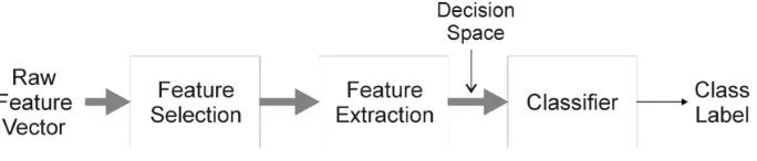
[image:3.595.137.479.354.427.2]Fig. 1 shows a prototypical pattern recognition system in which a vector of raw measurements is mapped into a decision space. Often the feature selection and/or extraction stages are either omitted or are implicit in the recognition paradigm a multi-layer perceptron (MLP)is a good example of a classification paradigm where a distinct feature extraction stage is not readily identifiable. Addison et al. [1] and Park et al. [2] have reviewed existing feature extraction and selection techniques while Guyon and Elisseeff [3] have discussed feature extraction in terms of filter and wrapper methods. In this paper we focus on feature extraction.
Figure 1: Prototypical pattern recognition system
The principal difficulty with designing the feature extraction stage for a classifier is that it usually requires deep domain-specific knowledge. (Indeed much of the work in image processing on detecting image cues such as edges and corners is actually feature extraction.) Even for feature extractors de-signed by domain experts, the issue of optimality is rarely addressed. Ideally, we would require some measure of class separability in the transformed de-cision space to be maximised but with handcrafted methods this is hard to guarantee.
In general terms, finding the optimal (possibly nonlinear) transformation,
criterion.
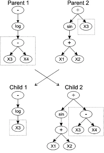
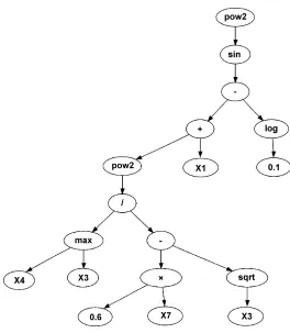
Genetic programming (GP) is an evolutionary problem solving method which has been extensively used to evolve programs or sequences of opera-tions [8]. Typically, a prospective solution in GP is represented as a parse tree which can be interpreted as a sequence of operations and thus evalu-ated. Fig. 2 shows example GP trees together with the crossover operation typically used in the search process; the the output of the tree on the left (Parent 1), for example, evaluates to the expression:
y=−log(X3−X4)
[image:4.595.218.392.305.562.2]where X3,4 are input features from the pattern being processed.
Figure 2: Illustration of the crossover operation in genetic programming
selected and replaced by a new, randomly-generated subtree. See Section 2.2 for details of the selection, crossover and mutation operations used in the present work. The cycle of selection/crossover/mutation is repeated either for a fixed number of iterations or until some some pre-specified error target is attained. (Genetic programming has been comprehensively reviewed in a recent book by Poli et al. [4]).
GP has been used before to optimise feature extraction and selection. Ebner [5, 6] has evolved image processing operators using GP. Bot [7] has used GP to evolve decision space features, adding these one-at-a-time to a kNN classifier if the newly evolved feature improved the classification performance by more than a certain amount. Bot’s approach is a greedy algorithm and therefore almost certainly sub-optimal. In addition, Koza [8] has produced character detectors using genetic programming while Tackett [9] evolved a symbolic expression for image classification based on image features.
Harvey et al. [10] evolved pipelined image processing operations to trans-form multi-spectral input synthetic aperture radar (SAR) image planes into a new set of image planes and a conventional supervised classifier was used to label the transformed features. Training data were used to derive a Fisher linear discriminant and GP was applied to find a threshold to reduce the output from the discriminant finding phase to a binary image. However, the discriminability is constrained in the discriminant finding phase and the GP only used as a one-dimensional search tool to find a threshold.
Sherrah et al. [11] proposed the Evolutionary PreProcessor (EPrep) sys-tem which used GP to evolve a good feature mapping by minimising misclas-sification error. Three typical classifiers: generalised linear machine (GLIM), k-nearest neighbour (kNN) and maximum likelihood classifiers were selected randomly and trained in conjunction with the search for the optimal fea-ture extractors. The misclassification errors on the validation set from those classifiers were used as a fitness value for the individuals in the evolution-ary population.The same procedure was used in the co-evolution of feature extraction/classifiers in [12]. This approach, however, makes the feature ex-traction procedure dependent on the classifier in an opaque way such that there is a potential risk that the evolved preprocessing can be excellent but the classifier can be poor giving a poor overall performance, or vice versa.
during the evolution. This protection method, however, contributes to the overfitting which is evident from his experiments. Indeed, Krawiec’s results show that for some datasets, the application of his feature extraction method actually produces worse classification performance than using the raw input data alone. Est´ebanez et al. [15] have followed a similar approach to Kraw-iec in projecting to a vector decision space of pre-determined dimensionality. Recently, Guo et al. [16] have evolved features in a condition monitoring task although it is not clear whether the elements in the vector of decision variables were evolved at the same time or hand-selected after evolution. Smith and Bull [17] have used GP together with a GA to perform feature construction and feature selection.
Broadly, the previous work on GP feature extraction can be categorised as evolving either: A discrete feature extraction stage which then feeds into a traditional classifier, or evolving a combined feature extraction/classification method which directly outputs a class label. Of the two possible routes, we argue that there is little merit in investing computational effort in evolv-ing classifiers since this area is well understood and has solid theoretical underpinnings. We argue that the available computational effort should be expended on producing good feature extraction; in addition, we question the speed of convergence when exploring a search space which contains not only the set of feature extractors but also the set of all classifiers. Consequently, we adopt the approach here of evolving optimal feature extraction algorithms and performing the classification task using a standard, simple and fast-to-train classifier since the classifier has to be included inside the evolutionary loop to evaluate an individuals fitness in terms of a separability measure in the decision space. We draw a distinction in the present work between evolv-ing a feature extraction stage and evolvevolv-ing a classifier since the outcome of our evolutionary optimisation is a mapping into a real-valued (1D) decision space, not a mapping into the space of object labels which is what would result from evolving a classifier. Clearly, our overall system does constitute a classification system and our feature extraction stages are conditioned on our choice of classifier, in the present case, a single threshold. As a future extension to the present framework, we envisage mapping the input patterns into a multidimensional decision space (see [11], for example) in which case the choice of classifier is explicitly much more open.
of standpoints. In particular, unless specific measures are taken to prevent it, the trees in a GP optimisation tend to grow without limit with no corre-sponding improvement in fitness, a phenomenon which is termed tree bloat. This is analogous to overfitting in neural networks and can lead to poor generalisation of the trained classifier as well as excessive computational de-mands. Various heuristic and indirect techniques have been used to suppress bloat but Ek´art and N´emeth [18] have shown that using a multiobjective fitness function [19] within GP, where one of the objectives is to minimise tree size, prevents bloat by exerting selective pressure in favour of smaller trees; also see [20].We have thus used a multiobjective framework with Pareto optimality [19] in the present work.
Rather than a single solution, the converged output of a multiobjective optimisation is a set of equivalent solutions whose members are superior to all the other feasible solutions; the members of this so-called Pareto set are said to dominate the other possible solutions [19]. Within this set, none can be considered better than any other from the point of view of the simultaneous optimisation of multiple objectives and it is left to a Decision Maker (DM) to select one of the optima according to some utility function which expresses their preferences. See [19] for a detailed review of multiobjective evolutionary methods; Jin and Sendhoff [21] have recently presented a review of Pareto-based multiobjective machine learning with particular emphasis on neural networks.
Our overall objective in the present work has been to identify the (near-) optimal series of mathematical transformations of pattern data that produces the best class separation in the transformed decision space. Further, our aim has been to produce a generic, domain-independent method such that the transformed patterns (or extracted features) can then be accurately classified with a simple and fast classifier.We make no assumptions about the statistical distributions of the original feature data.
For convenience and without loss of generality, we focus here on two-class problems. In common with other approaches to multi-two-class problems, extension to three or more classes is somewhat more involved and will be the subject of a future publication.
researchers.We offer conclusions and suggestions for future work in Section 4.
2. Methodology
Over the years much effort has been expended in the pattern recognition community on finding a best classifier(e.g. [23, 24]), the conclusion of which is that there is no single classifier which is best for every problem. In the present work,we focus on the feature preprocessing stage in classification systems. We propose a generic framework to evolve an optimal feature extraction stage for a given problem, independent of the dimensionality of the input pattern space and with optimised discriminability. If the optimisation is effective, patterns in the transformed space should not only be much easier to separate than the original pattern data but should also be optimal within the constraints imposed by the dimensionality of the decision space and the final classifier. By optimality, we mean here that our algorithm should, in principle, yield a classification performance which is comparable to the best of the set of all classifiers, thus doing away with the often lengthy process of determining which is the best classifier for a specific classification problem. Furthermore, the framework under discussion is not problem-specific and can be easily reused in other domains without or with simple modifications to the GP settings.
We perform the minimisation of vectors of (typically, competing) objec-tives using Pareto dominance – see [19] for a comprehensive review of evolu-tionary multiobjective optimisation. Given two objective vectors u,v∈RN,
u is said to dominate v, that is u≺ v:
u ≺v if f ∀i: 1. . . N ui 6vi ∧ ∃j : 1. . . N uj < vj
The Pareto dominance relation thus lays the foundation for comparisons between, and ranking of objective vectors in the evolutionary population.
2.1. Multiple Objectives
Tree complexity measurement: As pointed-out above, there is a danger that trees evolved by GP will become very large due to tree bloat.We have observed in early experiments without a complexity objective that huge trees could produce an extremely small error over the training set but a very poor error estimated over an independent validation set. Broadly, for a given training error, the simpler individual is preferred, an observation in accord with Ockham’s Razor. Thus we have used node count in the tree as a straightforward measure of tree complexity as one of our fitness vector elements driving the evolution. We thereby impose a selective pressure that favours small trees, all other things being equal.
Misclassification error: The second element we use in the fitness vector is the conventional one of the fraction of misclassified patterns counted over the training set,the so-called 0/1 loss.Since we are projecting the input pattern into a one-dimensional decision space we use a straight-forward, single threshold classifier where the threshold is adapted as part of the fitness value determination to give the minimum error. Taken over the whole training set, we find the optimal threshold for that particular mapping by performing a Golden Section search for the threshold value which minimises the misclassification rate, bracketed initially by the two extremal responses. The Golden Section search is terminated when there is no further improvement in the misclassifica-tion rate. Thus the training of the classifier is very fast and makes a negligible contribution to the time of a single iteration. The misclas-sification objective means we are trying to evolve a feature extractor which maps the original pattern space into a new feature space where thresholding is able to yield the smallest possible misclassification.
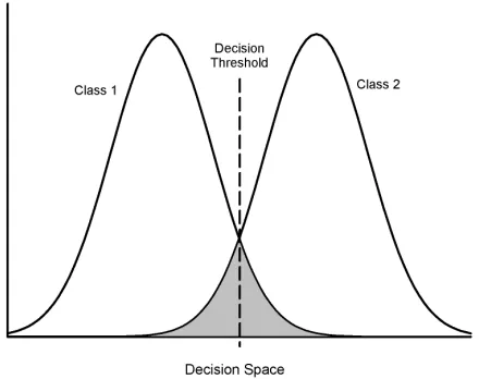
error from the overlap of the two histograms of the class-conditioned PDFs in the projected decision space; this is illustrated in Fig. 3. The Bayes error is a fundamental lower bound on classification performance in the decision space, dependent solely on the class-conditioned den-sities and independent of the classifier – see Fukanaga [25] for further details.
Figure 3: Illustration of the calculation of the Bayes error in the 1D Decision Space. The Bayes error is the overlap region between the two class-conditioned histograms (shown filled in grey).
The use of two measures of classification error the Bayes error estimate and the fraction of misclassified training set patterns requires further expla-nation. During our early experiments we found that using only the fraction of misclassified patterns (and the tree complexity measure) resulted in slow convergence and some cases, a failure to converge altogether. In the initial phases of the evolution when all the randomly-generated members of the population were typically poor performers, the misclassification error was close to its maximum. Consequently this objective lacked the sensitivity to identify individuals with slightly more promise than others, hence the poor convergence. In view of this we experimented with the alternative Bayes error measure.
es-timated validation error was disappointingly high. On closer inspection,it became clear that although the Bayes error objective was minimised over the training set, the GP was often opportunistically achieving this goal by producing two transformed class-conditioned densities in the decision space with non-coincident comb-like structures rather than the desired end of two compact densities with widely separated means. Consequently, although the degree of overlap of the likelihoods from the training set was small, the mis-classification error calculated over the validation set was large. This led us to using two error measures: the Bayes error allows the evolutionary search to make rapid progress in the initial stages of the optimisation while the frac-tion of misclassified patterns eventually comes to the fore when the evolufrac-tion advances to a certain stage of maturity and leads to two well-separated distri-butions. Overall, we have found experimentally that the combination of the three objectives is necessary for the algorithm to rapidly generate a Pareto set of parsimonious solutions which generalise well. Without the complexity measure the trees bloat and the optimisation tends to stagnate. Without the Bayes error objective, convergence is slow or non-existent. Each of the three objectives thus has a key role to play during the evolutionary pro-cess although since we are ultimately considering the classification domain, after we have generated a set of non-dominated solutions whose properties are ‘shaped’ by the multiple objectives,we select the solution which has the lowest (mean)validation error. This is a critical distinction between the cur-rent area and most other uses of multiobjective optimisation: The multiple objectives are vital constraints during the evolutionary process but after con-vergence, the nature of the problem does not actually form a conventional multiobjective trade-off.
2.2. MOGP Implementation
opposed to GA, methods based on the steady-state Pareto converging genetic algorithm (PCGA) [32] may confer some benefits for the present application in that PCGP appears able to produce smaller trees for a given misclassifica-tion error. The issue of comparisons between multiobjective GP algorithms is an area for future work.)
The SPEA-2 genetic programming implementation used here is a gen-erational strategy in which two sets of individuals are maintained during evolution. One set represents the current population and the second con-tains the current approximation to the Pareto front. The ranking is done by calculation of the strength, or fitness of each individual in both sets. When calculating the strength of an individual, we use the method proposed in SPEA-2 [20]. Here we make some modifications and reuse some strategies from SPEA/SPEA-2 to operate with genetic programming although we still store the non-dominated individuals in an external set, and cluster, if neces-sary. Using binary tournament selection we randomly select two parent trees for breeding from the union of the population and the non-dominated set. If both trees have been drawn from the same set we compare the normalised fitnesses to determine a winner; if not, we use the raw fitnesses to decide which should be chosen. We use non-destructive, depth-dependent crossover [33] and mutation operators in order to avoid the breaking of building blocks. We choose a subtree biased in its complexity (i.e. the number of nodes) using the depth-fair operator [33]; one of the subtrees at the chosen depth is then picked by roulette wheel selection, biased in its complexity. We initiate both genetic operations by randomly choosing a depth d ∈ [0. . . dmax] in a tree.
At the given depth d there areNd subtrees, each comprising M1, M2. . . MNd
nodes, respectively. The probability of selecting the i-th subtree is given by:
P r(i|d) = PNMi
d j=1Mj
and we select the target subtree using the standard roulette wheel approach. In the crossover operation we exchange the selected subtrees between the parents. In mutation, the selected subtree is replaced by a new, randomly created subtree attached at the selected mutation point. See [33] for further details.
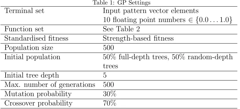
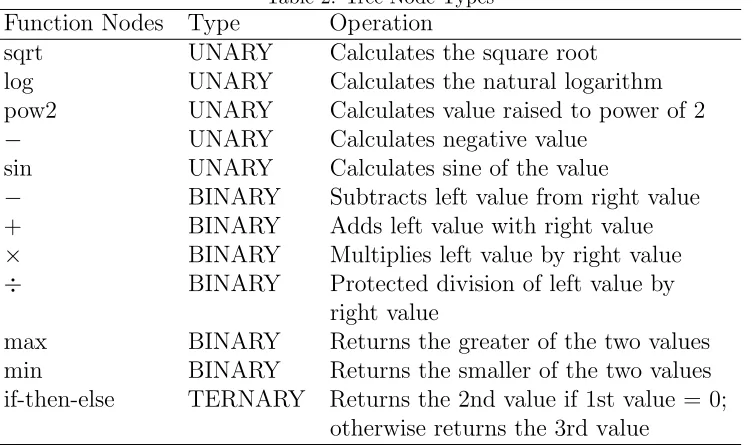
used in the GP implementation are listed in Table 1 and the function set used in the trees is detailed in Table 2.
Table 1: GP Settings
Terminal set Input pattern vector elements
10 floating point numbers ∈ {0.0. . .1.0} Function set See Table 2
Standardised fitness Strength-based fitness Population size 500
Initial population 50% full-depth trees, 50% random-depth trees
Initial tree depth 5 Max. number of generations 500 Mutation probability 30% Crossover probability 70%
The evolution was terminated when one of the following criteria was met: The misclassification error was zero, meaning all patterns in the training set are correctly labelled, OR the maximum number of generations was exceeded, OR the Bayes error of the best individual did not improve for some fraction of the maximum number of generations; we have used 0.04 as that fraction on the basis of experience although this number does not appear too critical.
3. Results
Table 2: Tree Node Types Function Nodes Type Operation
sqrt UNARY Calculates the square root log UNARY Calculates the natural logarithm pow2 UNARY Calculates value raised to power of 2 − UNARY Calculates negative value
sin UNARY Calculates sine of the value
− BINARY Subtracts left value from right value + BINARY Adds left value with right value × BINARY Multiplies left value by right value ÷ BINARY Protected division of left value by
right value
max BINARY Returns the greater of the two values min BINARY Returns the smaller of the two values if-then-else TERNARY Returns the 2nd value if 1st value = 0;
otherwise returns the 3rd value
the notion of optimality. We consider an extensive set of comparisons across eight 2-class learning problems. For each dataset we make a statistical com-parison of the classification performance between our MOGP algorithm and a range of established classifiers. If our conjecture about the generic power of our method is supported, then MOGP should perform at least as well as any other classifier (and in a number of cases,better).In addition, we com-pare where possible with previously reported evolutionary feature extraction techniques.
3.1. UCI and StatLog Datasets
The datasets used in the current work are:
1) Glass – 163 instances with nine attributes -This dataset has been con-verted to a two-class problem by seeking to distinguish between float glass and non-float glass.
2) BUPA Liver Disorders (BUPA) – Prediction of whether a patient has a liver disorder. There are two classes, six numerical attributes and 345 records.
4) Pima Indians Diabetes (PID) – Records with missing attributes were re-moved. This dataset comprises 532 complete examples with seven at-tributes.
5) Wisconsin Breast Cancer (WBC) – Sixteen of the instances with missing values were removed; 683 out of original 699 instances have been used here. Each record comprises ten attributes. This dataset has been used previously in [36].
6) Australian credit approval (AUS) – Credit card applications; comprises 690 instances in 14 attributes. 55.5% instances from positive decisions. This dataset has previously been investigated by Quinlan using decision trees [37].
7) Heart disease (HEA) – Contains 13 attributes, 270 samples. 120 samples present heart disease.
8) German credit (GER) – Classifies people described by 24 attributes as good or bad credit risks. 1000 instances, 700 of which are in good credit condition.
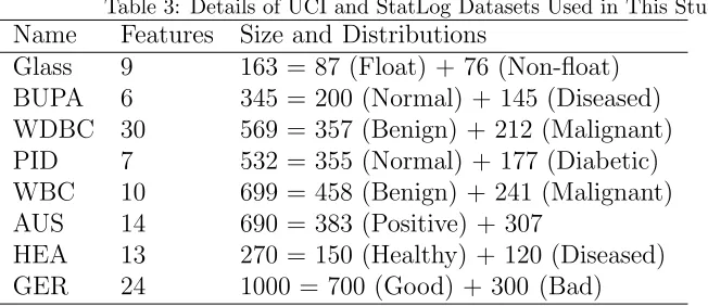
[image:15.595.111.437.424.565.2]For convenience, the details of the datasets used in the current work are summarised in Table 3.
Table 3: Details of UCI and StatLog Datasets Used in This Study Name Features Size and Distributions
Glass 9 163 = 87 (Float) + 76 (Non-float) BUPA 6 345 = 200 (Normal) + 145 (Diseased) WDBC 30 569 = 357 (Benign) + 212 (Malignant) PID 7 532 = 355 (Normal) + 177 (Diabetic) WBC 10 699 = 458 (Benign) + 241 (Malignant) AUS 14 690 = 383 (Positive) + 307
HEA 13 270 = 150 (Healthy) + 120 (Diseased) GER 24 1000 = 700 (Good) + 300 (Bad)
3.2. Comparator Classification Algorithms
from the Weka machine learning system2 [38] and we used the default
pa-rameter settings except where noted below. The classifiers used were:
1) Radial Basis Functions (RBF) – A normalised Gaussian radial basis func-tion network using the k-means clustering algorithm. We estimated the number of clusters (k) for a given dataset by considering a random split of the dataset, training the classifier on the first half and calculating a validation error on the second half. We adopted the value of k which gave the lowest validation error for each dataset by this method.
2) Logistic – Modified multinomial logistic regression model with a ridge estimator.
3) NNge – Nearest-neighbour-like algorithm using non-nested generalised ex-emplars.
4) BayesNet – Bayes Network classifier using the K2 learning algorithm. 5) IB1 – Instance-based learning algorithm. Uses a simple distance measure
to find the training instance closest to the given test instance and predict the same class as this training instance.
6) ADTree – The alternating decision tree learning algorithm.
7) SMO – Sequential minimal optimisation algorithm for training a support vector classifier.
8) C4.5 – The well-known decision tree algorithm. (This is referred to as J48 in Weka.)
In addition, we have used the classical Fisher Linear Discriminant (FLD) since comparative studies [24] show that this classifier is competitive across a wide range datasets. The version used here calculates the threshold assuming equal covariance Gaussian classes with a correction for the priors [39]; the priors were estimated from the dataset in question.
3.3. Comparison Methodology
Conventionally, classifiers have been compared in the literature using N-fold cross-validation followed by a t-test to gauge the statistical differ-ence between the results. Dietterich [40], however, has pointed-out this is unsound due to the implicit assumptions of independence being violated and has proposed an empirical 5 ×2 cv test. In turn, Alpaydin [41] has modified
2See:
http://www.cs.waikato.ac.nz/~ml/weka/. We have used Version 3.4.5 of
Dietterich’s test to remove the unsatisfactory aspect of the result depending on the ordering of the folds: it is Alpaydin’s F-test which we use here to statistically compare classifier performance.
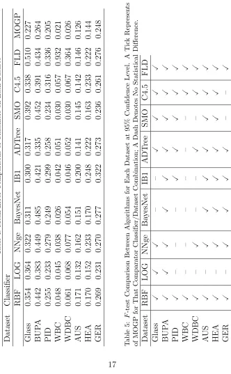
To compute the Alpaydin F-statistic we perform five repetitions of ran-domly splitting the dataset into two folds, treating one fold as a training set and the other as the test set. We then compute the F-statistic (see [41] for full details) and use this figure to decide whether or not to reject the null hypothesis that the performances of the two classifiers are identi-cal. Throughout this work we have used a 95% confidence level to infer a statistical difference which is equivalent to an F-measure > 4.74.
3.4. Comparisons with Conventional Classifiers
The outcome of the multiobjective optimisation is an approximation to the Pareto set, although as we explain in Section 2.1, the classification do-main does not constitute a trade-off in the conventional multiobjective sense. (Alternatively, the utility function which expresses the Decision Maker’s pref-erence [28] considers only the validation error to the exclusion of the other two objectives.) Therefore, to effect comparison of the classifier algorithms we have calculated the mean validation errors over the ten folds of the 5 ×2 cv test for each classifier, both evolutionary and conventional.
At the start of this Section we conjectured that the MOGP optimisations would yield classifiers which were either better than, or at worst, statistically identical to the best performing algorithm among the class of all classifiers. Clearly we are not able to prove such a conjecture as this would involve test-ing MOGP against the universe of all possible datasets with every possible classifier (including those as yet undiscovered). Nonetheless, we argue that the results presented here constitute strong evidence to support our conjec-ture.
As mentioned in Section 1, a number of other workers have explored (single objective) genetic programming to evolve either feature detectors or overall classifier systems. Muni et al. [42] have used GP to produce a c-class c-classifier (as distinct from a feature extraction stage) using a multi-tree representation. Bot [7] evolved new features which he added one-at-a-time until the improvement in classification performance dropped below a threshold. Bot and Langdon [43] produced linear classification trees using strongly typed GP. Loveard and Ciesielski [44] have explored five strategies for evolving classifiers while Krawiec [14] also constructed features using GP for subsequent classification with the C4.5 decision tree.
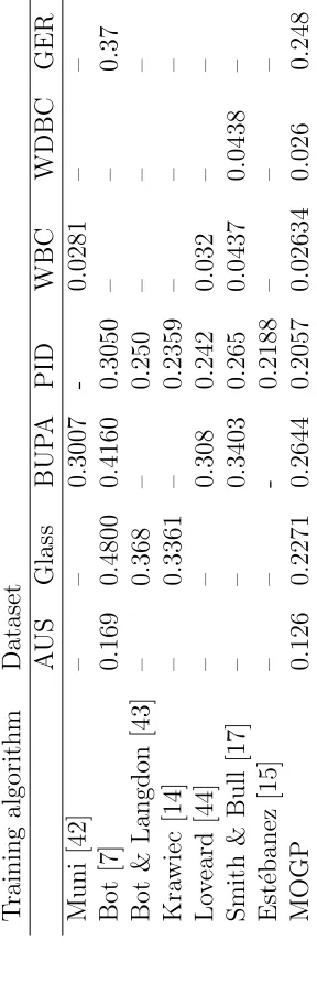
The error rates, where known, from these earlier studies are summarised in Table 6. Typically, error rates were the means estimated over ten-fold cross-validation. The results of Bot and Langdon [43] are the mean validation error of the best individual of 30 runs while those for Smith and Bull [17] are the best result from twenty repetitions with a 90%–10% partitioning of the dataset into training and test sets, respectively. In the case of the data of Loveard and Ciesielski [44], we show the most favourable results from the five strategies investigated by these authors. In the case of Est´ebanez et al. [15] we cite the average test error over five independent runs. Although in every case our MOGP method yields the lowest error rate, we are unable to assess the statistical significance of the differences in error rates on the basis of the published information. Nonetheless, the fact that MOGP records the lowest error rates is very promising and implies that MOGP is at very worst, equally good as the comparator evolutionary methods and quite possibly superior.
3.5. Interpretation of the Generated Trees
T able 6: Rep orted Error Rates for Other Ev olutionary Feature Detection/Classification Algorithms T raining algorithm
Dataset AUS
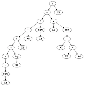
[image:20.595.241.385.248.694.2]objectives are important shaping forces during the evolution but do not form part of any ultimate design trade-off.) The terminal nodes displayed in the following tree graphs are labelled Xn wheren∈[1. . . N] denotes an element in the input pattern vector of dimensionality N.
Figure 4: MOGP transformation evolved for the PID dataset at generation 52
malignancy based on the Marginal Adhesion attribute alone thresholded at 3, we will obtain an error of 0.1399 assuming equal costs3. This is to be
compared with the error of 0.02634 obtained from the more complex tree shown in Fig. 7 which has a node count of 37. Nonetheless, it appears that the GP is eliciting sensible structure from this dataset – when (effectively) posed with the question of which is the best variable to use if constrained to just a single leaf, it correctly selects the most discriminatory.
Although one of our multiple objectives has been tree size, used to sup-press tree bloat, a number of the trees are not of the absolute minimum size and contain a few redundant subtrees. For example, Fig. 7 contains the sub-trees: max(0.5,0.8) which, of course, always returns the value of 0.8 as well as the subtreeif(0.1> 0) then X6 else X6 which always return the value of X6. We present the trees in Figs. 4 to 8 unedited since these are what have been generated by the evolutionary algorithm. It is clear, however, that these are not completely optimal in that the identical classification performance could be obtained in some cases with slightly smaller trees. Nonetheless, the work presented here produces near-optimal trees which are reasonable for a stochastic search method such as genetic programming and an advance on previous work on feature extraction. (In practice, any redundant subtrees could be easily removed from the final solution by hand if greatest model compactness was required.)
4. Conclusions and Future Work
In this paper we have demonstrated the use of multiobjective genetic pro-gramming (MOGP) to evolve an optimal feature extractor which transforms input patterns into a decision space such that class separability is maximised. In the present work we have projected the input pattern to a one-dimensional decision space since this transformation naturally arises from a genetic pro-gramming tree although potentially, superior classification performance could be obtained by projecting into a multidimensional decision space [11] this is currently an area of active research. What arises from our method is a fam-ily of equivalent solutions, the Pareto set, which simultaneously present the decision maker with the trade-off surface between training error and the com-plexity of the feature extractor; in the classification domain we will generally
3In medical diagnosis, equal costs are, of course, generally unacceptable; we use them
prefer the solution with the smallest 0/1 loss although this is not a neces-sary constraint. Although we effectively ignore two of the three objectives in selecting a final solution, the complexity and Bayes error objectives have a crucial role in rapidly shaping compact and by implication, well-generalising solutions.
A major objective in this work has-been to produce a domain-independent method and we have applied our algorithm to five machine learning tasks from the UCI database and three StatLog datasets. In comparison with a number of other representative classifier paradigms, the performance of our MOGP method turns-out to be better (or at worst, not statistically different). In no case was MOGP bettered by a conventional classifier which supports our conjecture that GP is finding the (near-)optimal feature extraction stage for a given classification problem.
The use of multiple objectives, particularly multiple classification error objectives has been shown to be effective in guiding and speeding the opti-misation. It is interesting that when only the Bayes error objective was used, GP was able to meet its goals of minimising the overlap of the two likelihoods in a way which was both unintended and unwanted. Clearly the intuitively straightforward concept of discriminability needs to be very carefully framed for use in an evolutionary setting to avoid the generation of opportunistic and unhelpful solutions.
Although we have treated only binary classification problems in this pa-per, extension to multiple classes is a logical development and is currently underway. Extension to large datasets is also a key issue where stochastic sub-sampling [45] may well prove a fruitful avenue.
[1] D. Addison, S. Wermter and G. Arevian, A comparison of feature extrac-tion and selecextrac-tion techniques, in Internaextrac-tional Conference on Artificial Neural Networks Supplementary Proceedings, Istanbul,Turkey (2003) pp. 212–215
[2] C. H. Park, H. Park and P. Pardalos, A comparative study of linear and nonlinear feature extraction methods, Technical Report TR 04-042, Department of Computer Science and Engineering, University of Min-nesota, Minneapolis, MN, 2004
[4] R. Poli, W. B .Langdon and N. F. McPhee, A Field Guide to Genetic Programming, Published via http://lulu.com and freely available at http://www.gp-field-guide.org.uk, 2008.
[5] M. Ebner, On the evolution of interest operators using genetic program-ming, in Late breaking papers in 1st European Workshop on Genetic
Programming, Paris, France (1998) pp. 610
[6] M. Ebner and A. Zell, Evolving a task specific image operator, in Joint Proceedings of the 1st European Workshop on Evolutionary Image
Anal-ysis, Signal Processing and Telecommunications (EvoIASP’99 and Eu-roEcTel’99), Goteborg, Sweden (1999) pp. 74–89
[7] M. J. C. Bot, Feature extraction for the k-nearest neighbour classifier with genetic programming, in EuroGP 2001, Lake Como, Italy, (2001) pp. 256–267
[8] J. R. Koza, Genetic Programming II: Automatic Discovery of Reusable Programs, MIT Press, Cambridge, MA, 1994.
[9] W. A. Tackett, Genetic programming for feature discovery and image discrimination, in 5th International Conference on Genetic Algorithms
(1993) pp. 303–309
[10] N. R. Harvey, J. Theiler, S. P. Brumby, S. Perkins, J. J. Szymanski, J. J. Bloch, R. B. Porter, G. Mark and A. Young, C, Comparison of GENIE and conventional supervised classifiers for multispectral image feature extraction, IEEE Transactions on Geoscience and Remote Sensing 40 (2002) 393–404
[11] J. R. Sherrah, R. E. Bogner and A. Bouzerdoum, The evolutionary preprocessor: Automatic feature extraction for supervised classification using genetic programming, in 2nd Annual Conference on Genetic
Pro-gramming, Palo Alto, CA (1997) pp. 304–312
[13] M. Kotani, M. Nakai and K. Azakawa, Feature extraction using evolu-tionary computation, in Congress on Evoluevolu-tionary Computation (1999) pp. 1230–1236
[14] K. Krawiec, Genetic programming-based construction of features for machine learning and knowledge discovery tasks, Genetic Programming and Evolvable Machines 3 (2002) 329–343
[15] C.Est´ebanez, R. Aler and J. M.Valls, A method based on genetic pro-gramming for improving the quality of datasets in classification prob-lems, International Journal of Computer Science and Applications 4 (2007) 69–80
[16] H. Guo, L. B. Jack and A. K. Nandi, Feature generation using genetic programming with application to fault classification, IEEE Transactions on Systems, Man and Cybernetics – Part B 35 (2005) 89–99
[17] M. G. Smith and L. Bull, Genetic programming with a genetic algo-rithm for feature construction and selection, Genetic Programming and Evolvable Machines 6 (2005) 265–281
[18] A. Ek´art and S. Z. N´emeth, Selection based on the Pareto nondom-ination criterion for controlling code growth in genetic programming, Genetic Programming and Evolvable Machines, 2 (2001) 61–73
[19] C. A. C. Coello, An updated survey of GA-based multiobjective opti-mization techniques, ACM Computing Surveys 32 (2000) 109–143
[20] S. Bleuler, M. Brack, L. Theile and E. Zitzler, Multiobjective genetic programming: Reducing bloat using SPEA2, in Congress on Evolution-ary Computation (2001) pp. 536–543
[21] Y. Jin and B. Sendhoff, Pareto-based multiobjective machine learning: An overview and case studies, IEEE Transactions on Systems, Man and Cybernetics – Part C 38 (2008) 397–415
[23] D. Michie, D. J. Spiegelhalter and C. C. Taylor, Machine Learning, Neu-ral and Statistical Classification, Ellis Horwood, Upper Saddle River, NJ, 1994
[24] T. Lim, W. Loh and Y. Shih, A comparison of prediction accuracy, complexity, and training time of thirty-three old and new classification algorithms, Machine Learning, 40 (2000) 203–228
[25] K. Fukunaga, Introduction to Statistical Pattern Recognition, 2nd ed.,
Academic Press, San Diego, CA, 1990
[26] C. Fonseca and P. J. Fleming, Multiobjective optimization and multiple constraint handling with evolutionary algorithms –Part I: A unified for-mulation, IEEE Transactions on Systems, Man and Cybernetics – Part A 28 (1998) 26–37
[27] K. Deb, A. Pratap, S. Agarawal and T. Meyarivan, A fast and elitist multiobjective genetic algorithm: NSGA-II, IEEE Transactions on Evo-lutionary Computing 6 (2002) 182–197
[28] A. Jaszkiewicz, Genetic local search for mullti-objective combinatorial optimization, European Journal of Operational Research 137 (2002) 50– 71
[29] J. D. Knowles, L. Thiele and E. Zitzler, A tutorial on the performance as-sessment of stochastic multiobjective optimizers, Technical Report TIK-214, Computer Engineering and Networks Laboratory, ETH, Zurich, Switzerland, 2005
[30] E. Zitzler and L. Thiele, An evolutionary algorithm for multiobjective optimization: The strength Pareto approach, Technical Report 43, Com-puter Engineering and Communications Networks Lab (TIK), Swiss Fed-eral Institute of Technology (ETH), Zurich, Switzerland, 1998.
[31] Y. Zhang and P. I. Rockett, A comparison of three evolutionary strate-gies for multiobjective genetic programming, Artificial Intelligence Re-views 27 (2007) 149–163
converging genetic algorithm, Evolutionary Computation 10 (2002) 283– 314
[33] T. Ito, H. Iba and S. Sato, Non-destructive depth-dependent crossover for genetic programming, in 1st European Workshop on Genetic
Pro-gramming, Paris, France (1998) pp. 14–15
[34] J. R. Koza, F. H. Bennett, D. Andre and M. A. Keane, Genetic Program-ming III: Darwinian Invention and Problem Solving, Morgan Kaufmann, San Francisco, CA , 1999
[35] O. L. Mangasarian, W. N. Street, and W. H. Wolberg, Breast cancer diagnosis and prognosis via linear programming, Operations Research 43 (1995) 570–577
[36] O. L. Mangasarian and W. H. Wolberg, Cancer diagnosis via linear programming, SIAM News 23 (1990) 1–18
[37] J. R. Quinlan, C4.5: Programs for Machine Learning, Morgan Kauf-mann, San Mateo, CA, 1993
[38] I. H. Witten and E. Frank, Data Mining: Practical Machine Learning Tools, 2nd ed., Morgan Kaufmann, San Francisco, CA, 2005
[39] R. O. Duda, P. E. Hart and P. E. Stork, Pattern Recognition, 2nd ed.
John Wiley and Son, New York, 2001
[40] T. Dietterich, Approximate statistical tests for comparing supervised classification learning algorithms, Neural Computation 10 (1998) 1895– 1923
[41] E. Alpaydin, Combined 5 ×2 cvF test for comparing supervised classi-fication learning algorithms, Neural Computation, 11 (1999) 1885–1892
[42] D. P. Muni, N. R. Pal and J. Das, A novel approach to design clas-sifiers using genetic programming, IEEE Transactions on Evolutionary Computation 8 (2004) 183–196
[43] M. J. C. Bot and W. B. Langdon, Application of genetic programming to induction of linear classification trees, in 11th Belgium/Netherlands
[44] T. Loveard and V. Ciesielski, Representing classification problems in genetic programming in Congress on Evolutionary Computation, Seoul, Korea (2001) pp. 1070–1077