This file is part of the following work:
Al-Juboori, Muqdad Raoof Kareem (2018)
Seepage criteria based optimal design
of water retaining structures with reliability quantification utilizing surrogate
model linked simulation-optimization approach.
PhD Thesis, James Cook
University.
Access to this file is available from:
https://doi.org/10.25903/5d815ed407a85
Copyright © 2018 Muqdad Raoof Kareem Al-Juboori.
The author has certified to JCU that they have made a reasonable effort to gain
permission and acknowledge the owners of any third party copyright material
included in this document. If you believe that this is not the case, please email
1
SEEPAGE CRITERIA BASED OPTIMAL DESIGN OF WATER
RETAINING STRUCTURES WITH RELIABILITY QUANTIFICATION
UTILIZING SURROGATE MODEL LINKED
SIMULATION-OPTIMIZATION APPROACH
A thesis submitted by
Muqdad Raoof Kareem Al-Juboori
2018
For the degree of Doctor of Philosophy (Ph.D.)
College of Science and Engineering
i
Statement of Access
I, the undersigned, author of this work, understand that James Cook University will make
this thesis available for use within the University Library and, via the Australian Digital Thesis
network, for use elsewhere.
I understand that, as an unpublished work, a thesis has significant protection under the
Copyright Act and I wish this work to be embargoed until September 2019, after which date I do
not wish to place any further restriction on access to this work.
Signature Date
Statement of Sources Declaration
I herewith declare that I have produced this thesis without the prohibited assistance of third parties
and without making use of aids other than those specified; notions taken over directly or indirectly
from other sources have been identified as such. This thesis has not previously been presented in
identical or similar form to any other Australian or foreign examination board.
Signature Date
Electronic Copy
I, the undersigned, the author of this work, declare that the electronic copy of this thesis provided
to James Cook University Library is an accurate copy of the print thesis submitted.
ii
Statement of Contribution of Others
All the prescribed methods, results and conclusions in the thesis were developed and written
by Muqdad Al-Juboori under complete supervision from my supervisor Dr. Bithin Datta. He
proficiently guided me for the entire PhD project, and provided me valuable recommendations to
overcome difficult challenges in my research. The material in the published articles in journals,
conference proceedings and the thesis was fulfilled by Muqdad Al-Juboori with important feedback
provided by Dr. Bithin Datta.
Financial contribution towards this PhD project was received from:
1. Iraqi Government and Ministry of Higher Education and Scientific Research
2. James Cook University- Australia, Graduate Research School and Collage of Science and Engineering.
iii
To My Mother (Alia Al-Ramahi)
To My Father (Raoof Al-Juboori)
To My Wife (Nawres Al-Yasiri)
To My Sons (Ali & Hussein)
To My Sisters (Nahid & Nabba)
To My Brothers (Ammar, Ahmed & Khalid)
I sincerely dedicate this thesis
iv
Acknowledgements
First and foremost, I thank the glorious creator of the universe, Allah almighty for granting me the ability and the strength to achieve this work.
I wish to express my deepest appreciation and thanks for my supervisor, Dr. Bithin Datta. He has supported and provided me valuable advices and academic guidance throughout my Ph.D. research tenure. His supervision aids me to defeat and overcome many obstacles faced in my research. The submission of this thesis has been possible due to his valuable feedbacks and continuous reviewing of my work and writing.
Thanks to the Iraqi Government and Iraqi Ministry of Higher Education and Scientific Research, for funding my scholarship, and to the Iraqi Embassy in Australia /Cultural Attaché, for looking after me during my study. Thanks for the James Cook University/ Australia, and the Graduate Research School, for providing the research requirements and the substantial support to participate in many conference s during my Ph.D. research. I also wish to extend my gratitude to Assoc. Prof. Siva Sivakugan, and other staff and colleagues in Collage of Science and Engineering. Also, I would like to extend the thanks to Geo-Studio/ SEEP/W, SIGMA/W and SLOPE/W team. They provided me the license to use this software in seepage modelling, and they responded to many technical inquires.
Finally, I cannot thank my wife, Nawres, enough for her support and encouragement to continue in my study and to defeat many problems during the past few years. Also, thanks for all my family, Mother, Father, sisters and brothers, for their support and pray to accomplish my degree. Also, I thank my sons, Ali and Hussein, they pushing me in their own ways toward the success. Lastly, I thank everybody who supported me even with a single word.
v
Publications Produced During Ph.D. Candidature
Peer-reviewed papers:
1. Al-Juboori, M & Datta, B. 2018 .Performance evaluation of a Genetic Algorithm based linked simulation-optimization model for optimal hydraulic seepage related design of concrete gravity dams. Journal of Applied Water Engineering and Research, Doi:10.1080/23249676.2018.1497558
2. Al-Juboori, M & Datta, B. 2018. Effects ofthe of the soil permeability on the optimum design of hydraulic water retaining structures utilizing support vector machine based linked simulation optimization models. KSCE Journal of Civil Engineer/ accepted 3. Al-Juboori, M & Datta, B. 2018. Linked simulation-optimization model for optimum
hydraulic design of water retaining structures constructed on permeable soils. International Journal of GEOMATE, Doi: 10.21660/2018.44.7229
4. Al-Juboori, M & Datta, B. 2018.optimum hydraulic design of concreter gravity dams founded on anisotropic soils utilizing interior point algorithm based hybrid genetic algorithm. ISH Journal of Hydraulic Engineering, under review
5. Al-Juboori, M & Datta, B. 2018.Reliability based optimum design of hydraulic water retaining structure constructed on heterogeneous porous media: utilizing stochastic. Life Cycle Reliability and Safety Engineering, under review
6. Al-Juboori, M & Datta, B. 2018. Incorporating uncertainty of heterogeneous hydraulic conductivity: utilizing stochastic ensemble surrogate models in objective multi-realization optimization model for optimum design of hydraulic water retaining structure. Journal of Computational Design and Engineering, under review.
Conference papers:
1. Al-Juboori, M & Datta, B .2017. Artificial Neural Network Modelling and Genetic Algorithm Based Optimization of Hydraulic Design Related to Seepage under Concrete Gravity Dams on Permeable Soils. The 19th International Conference on Environmental and Water Resources Engineering, Melbourne- Australia.
2. Al-Juboori, M & Datta, B .2017. Influence of hydraulic conductivity and its anisotropic ratio on the optimum hydraulic design of water retaining structures founded on
permeable soils. The 13th Hydraulics in Water Engineering Conference, Sydney – Australia.
vi
International Conference on Geo-technique, Construction Materials and Environment, Mie, Japan, Nov. 21-24, 2017, Mie- Japan.
vii
Nomenclature and Abbreviations
𝛾𝑠𝑢𝑏 Submerged soil density (kN/m3)
𝛾𝑤 Unite weight of water (kN/m3)
𝐺𝑆 Specific gravity of soil (kN/m3)
ANN Artificial neural network
b Width of HWRS (m)
B Total width of structures (m)
b* Part of the floor on upstream side of HWRS (m)
bi Width of the floor between cut-off (i) and (i+1), ∀ i, (m)
COV Coefficient of variation
CV Cross validation
DOE Design of experiment
d1 Upstream cut-off depths (m)
d2 Downstream cut-off depths (m)
e Eccentric load distance (m)
FEM Finite element method
Fovt Design safety factor against overturning
GA Genetic algorithm
GPR Gaussian process regression
H Total upstream hydraulic head or difference in elevation of water between upstream and downstream (m)
HC Hydraulic conductivity (m/day)
HHC Heterogeneous hydraulic conductivity
HS Halton sequences
viii
HWRS Hydraulic water retaining structure
ie Exit gradient
IPA Interior point algorithm
Ks Sliding safety factor
kx Hydraulic conductivity in horizontal direction
ky/kx Ratio of the hydraulic conductivity in y direction to the value of hydraulic conductivity in x direction
LD Soil layer depth (m)
LHS Latin hypercube sampling method
MAE Mean absolute error
MSE Mean square error
MOMRO Multi-objective multi-realization optimization
NSGA-II Non-dominated sorting genetic algorithm II
Pc1 Uplift pressure on upstream (kpa)
Pe2 Uplift pressure on downstream (kpa)
RBOD Reliability based optimum design
RSQ Coefficient of determination
S-O Simulation-optimization
SVM Support vector machine
ti Thickness of HWRS floor near the cut-off (i), ∀ i, (m)
βi Inclination angle of the cut-off (i), ∀ I, (degree)
γC Concrete weight density (kN/m3)
θC Uplift pressure at the upstream cut-off (kpa)
θE Uplift pressure at the downstream cut-off (kpa)
μ Mean of hydraulic conductivity (m/day)
ix
Abstract
The safety of hydraulic water retaining structures (HWRS) is an important issue as many instances of HWRS failure have been reported. Failure of HWRS may lead to catastrophic events, especially those associated with seepage failures. Therefore, seepage safety factors recommended for HWRS design are generally very conservative. These safety factors have been developed based on approximation calculations, unreliable assumptions, and ideal experimental conditions, which are rarely replicated in real field situations. However, with the development of the numerical methods, and high speed processors, more accurate seepage analysis has become possible, even for complex flow domains, different scenarios of boundary conditions, and varied hydraulic conductivity. On the other hand, because construction of HWRS requires a significant amount of construction material and engineering effort, the construction cost efficiency of HWRS is an issue that must be considered in design of HWRS.
This study aims to determine the minimum cost design of HWRS constructed on permeable soils, incorporating numerical solutions of a seepage system related to HWRS, utilizing linked a simulation–optimization (S-O) model. Due to the complexity and inefficacy of directly linking a simulation model to the optimization model, the numerical simulation model was replaced by trained surrogate models. These surrogate models can be trained based on numerically simulated data sets. Therefore, trained surrogate models expeditiously and accurately provide predicted responses relating to seepage characteristics pertaining to HWRS. The optimization model based on the linked S-O technique incorporated different safety factors and hydraulic structure design requirements as constraints. The majority of these constraints and objective function(s) were affected by the responses of predicted seepage characteristics based on the developed surrogate models.
To improve the safety of HWRS design, the effect of non-homogenous and anisotropic hydraulic conductivity were incorporated in the S-O model. Obtained solution results demonstrated that considering stratification of the flow domain due to different hydraulic conductivity values or anisotropic ratios can significantly change the optimum design of HWRS. Low hydraulic conductivity and anisotropic ratios resulted in more critical seepage characteristics. Consequently, the minimum construction cost increased due to an increase of dimensions of involved seepage protection design variables.
x
due to uncertainty of hydraulic conductivity was represented using many stochastic ensemble surrogate models. Each ensemble model included many surrogate models trained in utilizing input– output data sets simulated with different scenarios of hydraulic conductivity drawn from diverse random fields based on different log-normal distributions. Obtained results of this approach demonstrated substantial consequences of considering uncertainty in hydraulic conductivity. Also, the deterministic safety factors, especially for those pertaining to the exit gradient, were insufficient to provide prescribed safety in the long term.
Although surrogate models are utilized in S-O approaches, each run of the S-O model takes a long time as developed S-O models are applied to complex and large scale problems. Hence, efficiency of the S-O model was a key factor to successfully implement the methodology. Three main techniques were utilized to increase the efficiency of the S-O technique: using parallel computing, utilizing nested function technique, and using a vectorised formulation system. These strategies substantially boosted efficiency of implementing the S-O model.
The S-O models were implemented for many hypothetical scenarios for different purposes. In general, results demonstrated that optimum design of the seepage protection system relating to HWRS design must include two end cut-offs with an apron between them. The dimensions of these components were augmented with an increase of upstream water head, and reduction of anisotropic ratios or hydraulic conductivity value. The main role of the downstream cut-off was to decrease the actual exit gradient value. This impact is more pronounced if the inclination angle of the cut-off is toward the downstream side (>90 degrees). The role of the upstream cut-off was to decrease uplift pressure values on the HWRS base. Consequently, this partially contributed to decreasing the exit gradient value. The effect of the upstream cut-off in reducing the uplift pressure was more when the inclination angle was toward the upstream side (<90 degrees). Moreover, the apron (floor) width helped to increase the stability of HWRS. This variable provided the required weight to improve HWRS resistance to external hydraulic forces and to uplift pressure. Incorporating the weight of water (hydrostatic pressure) at the upstream side in counterbalancing momentum and hydraulic forces showed improvement in the safety of the HWRS. Also, all conditions and safety factors pertaining to HWRS design were satisfied. The exit gradient safety factor was the most important critical factor affecting optimum design as obtained optimum solutions satisfied the minimum permissible values of the exit gradient safety factor, i.e., at the minimum permissible value. Also, the eccentric load condition played a crucial role in resulting optimum solutions.
xi
xii
Table of Contents
Nomenclature and Abbreviations ... vii
Table of Contents ... xii
List of Tables ... xvii
List of Figures ... xix
1
Introduction ... 1
1.1 General Introduction ... 1
1.2 Problem Statement ... 4
1.3 Objectives of the Research ... 4
1.4 Organization of the Thesis ... 5
2
Theoretical Background and Literature Review ... 7
2.1 Earlier Empirical Seepage Analysis Methods for Hydraulic Structures ... 7
2.1.1 Bligh’s and Lane’s Theory ... 7
2.1.2 Khosla’s Theory ... 8
2.2 Approximate Solutions of Seepage ... 10
2.2.1 Fragment Method ... 10
2.2.2 Flow Net Method ... 11
2.3 Analytical Solution/Conformal Mapping by Schwarz-ChristoffelTransformation 11 2.4 Numerical Solution ... 13
2.4.1 Finite Element Method (FEM) ... 13
2.4.2 SEEP/W numerical seepage modeling and limited validation ... 15
2.5 Meta Model (Surrogate Model) ... 16
2.5.1 Artificial Neural Network (ANN) ... 17
xiii
2.5.3 Gaussian Process Regression (GPR) ... 19
2.5.4 Optimization Theory and the Application in HWRS ... 19
2.6 Linked Simulation Optimization (S-O) Model for HWRS design ... 21
2.7 Motivation and Scope ... 22
3
Performance Evaluation of Genetic Algorithm and Artificial Neural Network
Based Linked Simulation-Optimization Model for Optimal Design of Hydraulic
Water Retaining Structures ... 25
3.1 Introduction ... 25
3.2 Numerical Seepage Simulation Model Based on Finite Element Method (FEM) .. 27
3.3 Conceptual Seepage Model ... 28
3.4 Data Generation ... 30
3.5 ANN Description ... 30
3.5.1 Size of Training Data ... 32
3.5.2 Optimizing ANN performance ... 33
3.5.3 Cross validation ... 37
3.6 Optimization Model ... 38
3.6.1 Decision vector X ... 38
3.6.2 Objective function f (x) ... 39
3.6.3 Constraints defining simulated impact on the optimum design ... 40
3.6.4 Constraints defining design safety factors related to overturning, sliding, floatation, exit gradient and load eccentricity requirements ... 41
3.6.5 Genetic Algorithm (GA) ... 44
3.6.6 Maximizing GA performance ... 45
3.7 Results and discussion ... 48
3.7.1 ANN models ... 48
3.7.2 Simulation–Optimization model ... 50
xiv
3.7.4 The ANN model evaluation ... 54
3.7.5 S-O model evaluation ... 56
3.8 Conclusion ... 58
4
Coupled Simulation-Optimization Technique for Optimum Hydraulic Design of
Hydraulic Water Retaining Structures Constructed on Anisotropic and
Non-homogenous Permeable Soil ... 60
4.1 Introduction ... 60
4.2 Seepage conceptual model and data generation ... 61
4.3 Variable importance analysis ... 63
4.3.1 Variable importance analysis using Beta weight (standardized coefficient) .. 64
4.3.2 Variable importance analysis using Random Forest (RF) ... 65
4.3.3 Variable importance results and discussion ... 66
4.4 Support Vector Machine surrogate model ... 68
4.5 Optimization model ... 71
4.5.1 Formulation of the optimization model ... 71
4.6 Results and discussion ... 73
4.6.1 Head variation effects ... 73
4.6.2 Hydraulic conductivity (kx1) and anisotropic ratio (ky/ kx)1 effects ... 80
4.7 Conclusion ... 93
5
Global Optimum Hydraulic Design of Hydraulic Water Retaining Structures
Constructed On Anisotropic Permeable Soil Utilizing Interior Point Algorithm
Based Hybrid Genetic Algorithm ... 97
5.1 Introduction ... 97
5.2 Seepage conceptual model and data generation ... 98
5.3 Support vector machine surrogate model... 98
5.4 Optimization model ... 99
xv
5.4.2 Genetic algorithm ... 101
5.4.3 Hybrid genetic algorithm (HGA) ... 102
5.4.4 Formulation of the optimization model ... 103
5.5 Results and discussion ... 103
5.5.1 Optimization solvers efficiency ... 104
5.5.2 S-O solutions result ... 106
5.5.3 Optimum solution evaluations ... 109
5.6 Conclusion ... 113
6
Reliability Based Optimum Design of Hydraulic Water Retaining Structure
Constructed on Heterogeneous Porous Media: Utilizing Stochastic Ensemble
Surrogate Model Based Coupled Simulation Optimization Model ... 115
6.1 Introduction ... 115
6.2 Conceptual seepage model and design of experiments ... 118
6.3 Gaussian process regression (GPR) model ... 124
6.3.1 Gaussian process for regression ... 124
6.3.2 Surrogate model performance ... 126
6.4 Formulating the reliability based optimization model ... 130
6.5 Computational efficiency of the S-O model ... 132
6.6 Results and discussion ... 133
6.7 Evaluation of results ... 138
6.8 Conclusion ... 140
7
Optimum Design of Hydraulic Water Retaining Structures
Incorporating
Uncertainty in Estimating Heterogeneous Hydraulic Conductivity Utilizing
Stochastic Ensemble Surrogate Models within Multi-Objective Multi-Realization
Optimization Model ... 143
7.1 Introduction ... 143
7.2 Linked simulation–optimization (S-O) model ... 145
xvi
7.4 Design and evaluation of surrogate models ... 148
7.5 Multi-objective multi-realization optimization model ... 151
7.6 Non-dominated sorting genetic algorithm-II (NSGA-II) ... 152
7.7 Formulation of the reliability based MOMRO model ... 154
7.8 Computing efficiency... 158
7.9 Results and discussion ... 159
7.10Evaluation of the methodology ... 167
7.11Conclusion ... 170
8
Summary and conclusion ... 172
8.1 Summary ... 172
8.2 Conclusion ... 174
8.3 Limitations ... 176
8.4 Recommendations for future studies ... 177
9
References ... 178
10
Appendix A ... 189
xvii
List of Tables
Table 3.1 Assumed range of input variables ... 28
Table 3.2 Taguchi Orthogonal Array Design L16 (4^4) with S/N ratio ... 35
Table 3.3 Conformation experiments for different levels of C1, C2, D2 and D3 for θC ANN model ... 35
Table 3.4 Cross valuation results for different training / testing sets ... 38
Table 3.5 Taguchi DOE for GA parameters with normalized fitness value for different head values... 46
Table 3.6 Comparison of the objective function values obtained by improved GA model and the MATLAB default parameter model. ... 48
Table 3.7 Description of the developed ANN models ... 48
Table 3.8 ... 53
Table 3.9 Evaluation of S-O optimum solutions with SEEP/W and Khosla’s solutions ... 58
Table 4.1 Statistical description of the generated data ... 63
Table 4.2 Appearance of the important variables in the PEi model ... 67
Table 4.3 Appearance of the important variables in the PCi model... 67
Table 4.4 Final combination of predictors for each seepage characteristic ... 68
Table 4.5 Safety factors for different values of H ... 75
Table 4.6 Safety factors for the implemented cases for different kx1 ... 82
Table 4.7 Safety factors for the implemented cases for different (ky/kx)1 ... 83
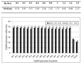
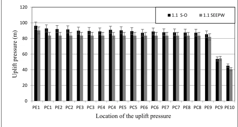
Table 4.8 Mean absolute error for predicted uplift pressure at specified locations of HWRS for different (kx)1 ... 86
Table 4.9 Mean absolute error for predicted uplift pressure at specified locations of HWRS for different (ky/kx)1 ... 87
Table 5.1 Formulation for the interior point algorithm ... 99
Table 5.2 Options and parameter values for GA and IPA ... 104
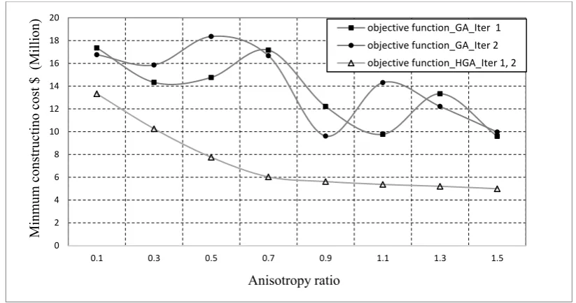
Table 5.3 Objective function values obtained by HGA and GA for different ky/kx ratio ... 105
Table 5.4 Performance efficiency of HGA and GA (ky/kx=1.5) ... 106
Table 5.5 Stopping condition and objective function values of IPA... 106
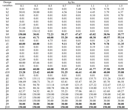
Table 5.6 Optimum solutions based on HGA ... 107
Table 5.7 Safety factors for the optimum solution for different ky/kx ratios... 108
Table 6.1 Properties of the GPR technique ... 126
Table 6.2 Samples of surrogate model training testing error measures ... 128
Table 6.3 Evaluation results for four randomly selected optimum solutions ... 140
Table 7.1 Parameters of the GPR technique ... 148
xviii
Table 7.3 Utilized NSGA-II parameters for the MOMRO model ... 154
Table 7.4Different optimum solution values for same objective functions values obtained by NSGA-II ... 164
Table 7.5 Minimum and maximum feasible solutions for different reliability level (H=100 m) ... 165
Table 7.6 Minimum and maximum feasible solutions for different reliability level (H=80 m) ... 165
Table 7.7Minimum and maximum feasible solutions for different reliability level (H=60 m) ... 166
Table 7.8 Minimum and maximum feasible solutions for different reliability level (H=40 m) ... 166
Table 7.9 Minimum and maximum feasible solutions for different reliability level (H=20 m) ... 167
Table 7.10 Evaluation results for case A (COV=147.5%) ... 168
Table 7.11 Evaluation results for case B (COV=112.5%) ... 169
Table 7.12 Evaluation results for case C (COV=182.5%) ... 169
xix
List of Figures
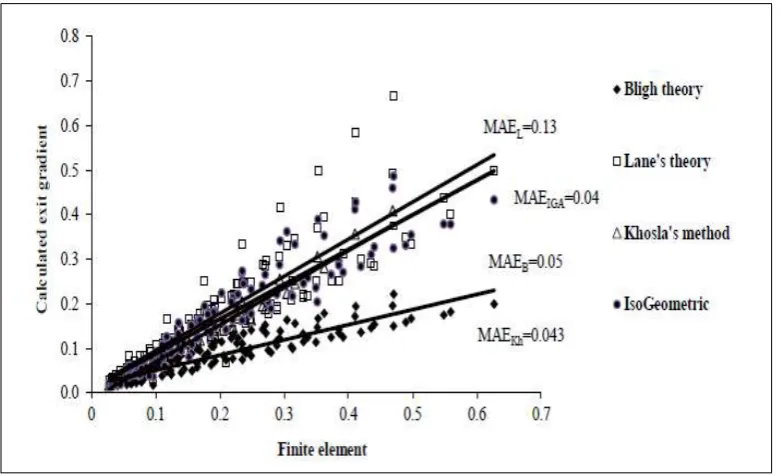
Figure 1.1 Comparing computed exit gradient by different methods and FEM based numerical solutions
(Shahrbanozadeh, Barani, & Shojaee, 2015) ... 2
Figure 2.1 One cut-off with apron (Khosla et al., 1936) ... 9
Figure 2.2 Validation of the SEEP/W solutions (uplift pressure) ... 16
Figure 2.3 Validation of the SEEP/W solutions (Exit gradient) ... 16
Figure 3.1 Conceptual seepage model ... 28
Figure 3.2 Comparing effect of soil layer depth to HWRS width on total head ratio (Harr, 1962) ... 29
Figure 3.3 Effect of the cut-off embedment length on normalized discharge (q/kh) (Harr, 1962) ... 29
Figure3.4 Typical ANN architecture ... 30
Figure 3.5 Standardized and standard deviation error for θC ANN model with different training/testing data size ... 32
Figure 3.6 Standardized and standard deviation error for θE ANN models with different training/testing data size ... 33
Figure 3.7 Standardized and standard deviation error for exit gradient ANN model with different training/testing data size ... 33
Figure 3.8 Main effects SN ratio (larger is better) of the θC ANN model ... 36
Figure 3.9 Main effects SN ratio (larger is better) of the θE ANN model ... 36
Figure 3.10 Main effects SN ratio (larger is better) of the exit gradient ANN model ... 37
Figure 3.11 General schematic of the linked simulation-optimization model ... 40
Figure 3.12 Free body diagram of the HWRS ... 44
Figure 3.13 Main effects SN ratio (small is better) for GA parameters ... 47
Figure 3.14 Chart for estimating the exit gradient based on the developed ANN model as a fraction of total head, α=2b/d1 ... 49
Figure 3.15 Chart for estimating the uplift pressure (θE) based on the developed ANN model as a fraction of total head, α=2b/d1 ... 49
Figure 3.16 Chart for estimating the uplift pressure (θC) based on the developed ANN model as a fraction of total head, α=2b/d1 ... 50
Figure 3.17 Optimum solution (d1, d2, 2b, b*, t1, t2) for different head values ... 51
Figure 3.18 Comparison of ANN solution with SEEP/W and Khosla’s solutions (Exit gradient) ... 55
Figure 3.19 Comparison of ANN solution with SEEP/W and Khosla’s solutions (θC) ... 55
Figure 3.20 Comparison of ANN solution with SEEP/W and Khosla’s solutions (θE) ... 55
xx
Figure 3.22 Comparison of seepage characteristics (θE) of the optimum obtained by S-O model, Numerical model (SEEP/W) and Khosla’s theory ... 57 Figure 3.23 Comparison of seepage characteristics (Exit gradient) of the optimum obtained by S-O model, Numerical model (SEEP/W) and Khosla’s theory ... 57 Figure 4.1 Seepage conceptual model scheme ... 62 Figure 4.2 Linear separation support vector (two classes) ... 69 Figure 4.3 Optimum width between cut-offs of the implemented cases for different head values ... 74 Figure 4.4 Optimum cut-off depths for the implemented cases for different head values ... 75 Figure 4.5 Optimum location of load resultant (R) for different values of head ... 76 Figure 4.6 Minimum cost optimum design of HWRS for different values of head ... 77 Figure 4.7 Optimum floor thickness of HWRS for different values of head ... 77 Figure 4.8 Evaluation results for different locations of uplift pressure (H=100 m) ... 78 Figure 4.9 Evaluation results for different locations of uplift pressure (H=80 m) ... 79 Figure 4.10 Evaluation results for different locations of uplift pressure (H=60 m) ... 79 Figure 4.11 Evaluation results for different locations of uplift pressure (H=40 m) ... 79 Figure 4.12 Evaluation results for different locations of uplift pressure (H=20 m) ... 80 Figure 4.13 Comparison of exit gradient of the optimum design to the numerical solution ... 80 Figure 4.14 Minimum cost for optimum design of HWRS for different values of kx1 ... 81
Figure 4.15 Minimum cost for optimum design of HWRS for different values of (ky/kx)1 ... 81
Figure 4.16 Resultant(R) location for different values kx1 ... 83
Figure 4.17 Resultant (R) location for different (ky/kx)1 values ... 83
Figure 4.18 Optimum width between cut-offs of HWRS for different values kx1 ... 84 Figure 4.19 Optimum cut-off depths of HWRS for different values kx1 ... 85 Figure 4.20 Optimum width between cut-offs of HWRS for different values (ky/kx)1 ... 85
Figure 4.21 Optimum cut-off depths for different values (ky/kx)1 ... 85
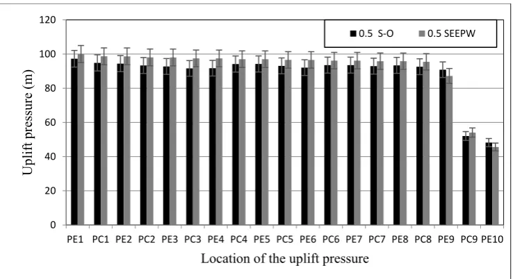
Figure 4.22 Evaluation results for different locations of uplift pressure (kx1=0.1 m/day) ... 87 Figure 4.23 Evaluation results for different locations of uplift pressure (kx1=0.1 m/day) ... 87 Figure 4.24 Evaluation results for different locations of uplift pressure (kx1=0.1 m/day) ... 88 Figure 4.25 Evaluation results for different locations of uplift pressure (kx1=0.1 m/day) ... 88 Figure 4.26 Evaluation results for different locations of uplift pressure (kx1=0.1 m/day) ... 88 Figure 4.27 Evaluation results for different locations of uplift pressure (kx1=0.1 m/day) ... 89 Figure 4.28 Evaluation results for different locations of uplift pressure (kx1=0.1 m/day) ... 89 Figure 4.29 Evaluation results for different locations of uplift pressure (kx1=0.1 m/day) ... 89 Figure 4.30 Evaluation results for different locations of uplift pressure (kx1=0.1 m/day) ... 90 Figure 4.31 Evaluation results for different locations of uplift pressure (kx1=0.1 m/day) ... 90 Figure 4.32 Evaluation results for different locations of uplift pressure ((ky/kx)1=0.1) ... 90
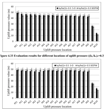
Figure 4.33 Evaluation results for different locations of uplift pressure ((ky/kx)1=0.3) ... 91
xxi
Figure 4.35 Evaluation results for different locations of uplift pressure ((ky/kx)1=0.7) ... 91
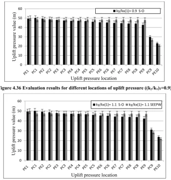
Figure 4.36 Evaluation results for different locations of uplift pressure ((ky/kx)1=0.9) ... 92
Figure 4.37 Evaluation results for different locations of the uplift pressure ((ky/kx)1=1.1) ... 92
Figure 4.38 Evaluation results for different locations of uplift pressure ((ky/kx)1=1.3) ... 92
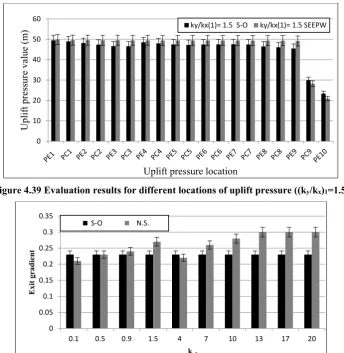
Figure 4.39 Evaluation results for different locations of uplift pressure ((ky/kx)1=1.5) ... 93
Figure 4.40 Exit gradient evaluation results for different values of (kx1) ... 93 Figure 4.41 Exit gradient evaluation results for different values of (ky/kx)1 ... 93
Figure 5.1 Conceptual seepage model ... 98 Figure 5.2 Objective function by HGA and GA ... 105 Figure 5.3 Load resultant location (e) ... 108 Figure 5.4 Evaluation results for different locations of the uplift pressure (ky/kx =0.1) ... 110 Figure 5.5 Evaluation results for different locations of the uplift pressure (ky/kx =0.3) ... 110 Figure 5.6 Evaluation results for different locations of the uplift pressure (ky/kx =0.7) ... 111 Figure 5.7 Evaluation results for different locations of uplift pressure (ky/kx =0.9) ... 111 Figure 5.8 Evaluation results for different locations of uplift pressure (ky/kx =1.1) ... 111 Figure 5.9 Evaluation results for different locations of uplift pressure (ky/kx =1.3) ... 112 Figure 5.10 Evaluation results for different locations of uplift pressure (ky/kx =1.5) ... 112 Figure 5.11 Exit gradient evaluation for different anisotropic ratios ... 112 Figure 6.1 Conceptual model of HWRS ... 120 Figure 6.2 Random data sampling using a) HS method b) LHS method for width of HWRS [b (0-150) m]121 Figure 6.3 Log-normal histogram for a sample of (μ = 2, σ = 0.85) ... 122 Figure 6.4 Different realizations of hydraulic conductivity for same standard deviation value ... 122 Figure 6.5 Effect of different realizations (for same σ value) of hydraulic conductivity variation on exit gradient contour ... 123 Figure 6.6 Training-testing R index for the surrogate model (ie3) (STD=2.25 m/day) ... 128
Figure 6.7 Training-testing R index for the surrogate model (ie4) (STD = 2.25 m/day) ... 128
Figure 6.8 Training-testing R index for the surrogate model (PC1) for (STD=2.25 m/day) ... 128
Figure 6.9 Training-testing R index the surrogate model (PE2) (STD = 2.25 m/day) ... 128
Figure 6.10 ie2 surrogate model prediction for test data (STD = 2.95 m/day) ... 129
Figure 6.11 ie1 surrogate model prediction for test data (STD = 2.95 m/day) ... 129
Figure 6.12 Illustrative formulation of reliability based stochastic S-O model ... 132 Figure 6.13 Optimum cost of HWRS for different reliability levels and different head values... 134 Figure 6.14 Optimum length of upstream cut-off (d1) for different reliability levels and different head values
... 136 Figure 6.15 Optimum length of downstream cut-off (d2) for different reliability levels and different head values
xxii
Figure 6.18 Sample of surrogate model (ie1) prediction from different stochastic surrogate models ... 138
Figure 7.1 Conceptual model of the HWRS ... 146 Figure 7.2 A randomly selected case, including different realizations of HHC (A1, A2) drawn from the same
log-normal distribution (µ=2, σ=3.65). B1, B2 represent effect of the different realization of HHC (A1, A2) on
the exit gradient distribution. C1, C2 represent effect of the different realization of HHC (A1, A2) on total head
distribution ... 147 Figure 7.3 ie4 surrogate model prediction for test data (σ=2.95-D*) ... 149
Figure 7.4 Pc1 surrogate model prediction for test data (σ=3.65-D) ... 149 Figure 7.5 Training-testing R index for the surrogate model (ie4) (σ=2.25-C ) ... 149
Figure 7.6 Training- testing R index for the surrogate model (ie2) (σ=3.65-B) ... 150
Figure 7.7 ie2 surrogate model training performance (σ=2.95-A) ... 150
1
1
Introduction
1.1
General Introduction
Construction of hydraulic water retaining structures (HWRS), such as dams, barrages, regulators and weirs, is essential for stable and safe water management and to generate clean energy. Future projections of water resources indicate that water availability will significantly decrease for several countries around the world (Gerten et al., 2011). This may be attributed to climate change and carbon dioxide (greenhouse gas) emissions due to human activities. Building HWRS is a beneficial and important solution to reduce the impacts of water scarcity. However, significant considerations and hazards must be considered in design of HWRS. The economic cost of building such projects is enormous; additionally, failures of HWRS threaten human life and properties on downstream. Accordingly, the design and analysis of such structures must involve precise estimation and sufficient understanding of the influencing design variables and parameters, especially the seepage quantities and their impacts on safety of HWRS. This study presents coupled simulation-optimization (S-O) approaches to identify the minimum cost HWRS design, incorporating numerical seepage analysis and considering the hydraulic design safety factors in S-O models. Furthermore, the effects of permeability (hydraulic conductivity) and its uncertainty are integrated in S-O models. The numerical seepage simulation is indirectly linked to the optimization model using machine learning techniques based on surrogate models. Artificial neural network (ANN), support vector machine (SVM) and Gaussian process regression (GPR) machine learning techniques were used to develop surrogate models. The genetic algorithm (GA), hybrid genetic algorithm (HGA) and non-dominated sorting genetic algorithm II (NSGA-II) were utilized to solve optimization tasks due to the complexity and the attribute of each S-O model.
2
pressure, which applies uplift (upward) pressure on the structure floor (apron) and may result in collapse of the floor.
[image:27.595.104.496.410.648.2]The hydraulics of seeping water and associated mathematical relationship of seepage variables with flow domain characteristics is complex and nonlinear. The complexity arises from many factors, such as sub-structure geometry, soil properties and hydraulic conductivity variation and uncertainty. An analytical solution may be obtained only for simple and symmetrical cases and is often based on assumptions that are not always correct. However, it is difficult to obtain analytical solutions for more complex scenarios, which occur in most of existing projects. Therefore, many approximation and empirical theories have been proposed to estimate seepage quantities (uplift pressure and exit gradient). These theories include Bligh’s creep theory, Lane’s weighted creep theory, flow-net method, fragment method and Khosla’s theory. Solutions of these approximate theories are acceptable to some extent. Their applications have an associated non-trivial amount of error compared to applications that use analytical solutions or experimental modelling, as shown in Figure1.1. Additionally, these theories apply to ideal general soil conditions (homogeneous and isotropic), which are rarely found in real life cases (Lambe & Whitman, 1969). Also, it is not possible to integrate the effects of hydraulic conductivity and uncertainty when utilizing these methods and theories.
Figure 1.1 Comparing computed exit gradient by different methods and FEM based numerical solutions (Shahrbanozadeh, Barani, & Shojaee, 2015)
3
methods, such as finite element method (FEM) and finite difference method (FDM). The FEM and FDM are the dominant numerical methods in this field. These methods provide accurate and efficient results even for complex problems. Consequently, many software and codes have been developed to facilitate numerical simulation of seepage problems, particularly after development of high-speed computer processors. These codes can be used to analyse complex seepage problems precisely. Furthermore, hydraulic conductivity variation and other soil parameters can be integrated in the numerical model to study consequences of soil parameter variation on HWRS design. However, a source of weakness of using numerical solutions is that the numerical technique only provides a solution for predetermined problems, including pre-defined boundary conditions and geometry of the flow domain of hydraulic structures. This means the numerical model may not provide a generalized performance equation regarding what can be obtained by analytical solution.
Considering the above-mentioned arguments, contradicting goals of safety and cost must be simultaneously integrated in design of HWRS to attain optimum, safe and economic design based on accurate seepage numerical solutions. Hence, the optimization approach can be used to identify optimal design of HWRS. As a result, the minimum cost and safest HWRS can be achieved. Directly integrating the numerical model with the optimization model to attain an optimum HWRS design is computationally inefficient, a computational burden and time consuming task. Also, most evolutionary optimization algorithms (solvers) utilize direct search techniques based on a large population size. These optimization solvers present many random candidate solutions (individuals) and evaluate each single solution based on numerical seepage responses for that solution. This optimization process and others continue for many generations until the stopping criteria is met. Accordingly, directly linking the optimization model to the simulation model is a complex and computationally expensive process. Alternatively, the numerical model could be replaced by an approximate machine learning model (surrogate model) that accurately and expeditiously imitates numerical model responses. The surrogate model may be trained based on numerically simulated data (input and output) sets. There are many machine learning techniques that can be utilized to develop a surrogate mode, such as artificial neural network (ANN), support vector machine and Gaussian process regression (GPR).
4
of HWRS. The uncertainty and spatial variation of hydraulic conductivity are considered in optimum design of HWRS. Identifying the most important design variable in optimum design is another goal of this study. Also, computational efficiency of the developed methodology is a significant aspect that must be considered in developing S-O techniques. Induced seepage forces and many safety factors and design requirements related to HWRS, such as overturning, sliding safety factors and preventing the eccentric load condition, are considered in the S-O approaches. For each S-O model, the type of machine learning technique and optimization solver are selected based on prediction accuracy and efficiency.
1.2
Problem Statement
The relationship between seepage design variables related to HWRS is usually categorized as a high degree nonlinearity problem, especially for complex problems (Harr, 1962). Many existing hydraulic structures built with high cost suffered from seepage problems, which may lead to failure of the structure. Such problems may be attributed to the approximation methods and theories by which the seepage related structures were analysed. Furthermore, these theories disregard spatial variation and uncertainties in some parameters, such as hydraulic conductivity, which have a significant effect on seepage characteristics. Providing a safe exit gradient for HWRS based on accurate and reliable analysis reduces actual possibility of piping failure. Also, decrease in the uplift pressure impacts provide a safer HWRS design. Moreover, construction of HWRS requires a considerable amount of construction materials and engineering effort, resulting in higher construction cost. Also, the HWRS safety design requirement must be simultaneously considered in HWRS design. Hence, there is a knowledge gap in obtaining optimum design for HWRS, which is partially filled by this research via developing a linked S-O model to determine minimum cost and safe design of HWRS by integrating numerical responses. These responses are based on trained surrogate models adequately trained and validated using numerically simulated data sets.
1.3
Objectives of the Research
The main objectives of this research are:
1. Develop and evaluate a coupled S-O model to obtain optimum design of HWRS founded on homogenous isotropic permeable soils and including a variable flat apron (floor) with variable length cut-offs.
5
3. Enhancing the performance of the S-O model by hybridizing the genetic algorithm with the interior point algorithm to attain a global optimum solution of multiple cut-offs multi aprons seepage flow domain under HWRS constructed on homogenous anisotropic permeable soil.
4. Develop stochastic ensemble surrogate models to incorporate various uncertainties to develop reliability based optimum design (RBOD) framework to determine the reliable and optimum design of HWRS founded on heterogeneous isotopic permeable soil, and including and a flat apron with end cut-offs.
5. Develop a multi-objective multi-realization optimization model for reliability based optimum design framework to find a reliable and optimum design of HWRS founded on heterogeneous isotropic permeable soils.
1.4
Organization of the Thesis
The thesis contains eight chapters, encompassing the current (Introduction) chapter. The introduction chapter provides a brief description of the main effects of seepage quantities on the HWRS design. The chapter includes an overview of the utilized methodology to find the optimum design and to incorporate the numerical seepage responses based on surrogate models in the S-O model. The problem statement and objective of the study are also presented in this chapter.
Chapter two provides a review of literature starting with earliest methods related to seepage analysis of HWRS. Also, important previous studies utilizing numerical methods for seepage solution are briefly discussed. The chapter cites previous research which incorporates optimization models to improve HWRS design. This chapter also highlights the contribution of machine learning techniques in enhancing understanding of relationships between design variables of HWRS. Additionally, machine learning technique applications in predicting the future behaviour or consequences for a particular design of HWRS are presented.
6
Chapter four contains the formulation of the linked S-O model to attain the optimum design of HWRS comprising of many cut-offs and aprons between them. The effects of non-homogenous anisotropic hydraulic conductivity are incorporated in the S-O model. Development of surrogate models was based on the support vector machine (SVM) technique, and the optimization model was based on the hybrid genetic algorithm (HGA). The optimum solution obtained via the S-O model and evaluation of S-O models are also included in this chapter.
Chapter five demonstrates the efficiency of hybridizing the genetic algorithm with the gradient search algorithm to achieve the global optimum solution within the linked S-O technique. Description and formulation of the optimization model are demonstrated in this chapter. The conceptual model of seepage includes many cut-offs, many aprons and homogenous anisotropic permeable flow domain. The SVM technique was utilized to develop the surrogate models. The safety factors and HWRS design requirements are included, with the results and performance evaluation of the S-O model presented in this chapter.
Chapter six encompasses formulation of the reliability based optimum design of HWRS. This was achieved by developing many ensemble surrogate models to incorporate stochastic responses of seepage characteristics due to uncertainties in estimating hydraulic conductivity in the linked S-O model. The surrogate models were developed based on the Gaussian progress recession (GPR) technique and the optimization solver was the genetic algorithm (GA). Hydraulic conductivity was represented as a random field sampled from a log-normal distribution based on different standard deviation values. Solution results and performance evaluation of the developed methodology are included in this chapter.
Chapter seven presents a new formulation of the reliability based optimum design utilizing the multi-objective, multi-realization optimization model based on the ensemble surrogate models. Many ensemble surrogate models were developed to represent the stochastic responses of seepage characteristics due to uncertainty in estimation of hydraulic conductivity. The conceptual model included an apron between two end cut-offs. Hydraulic conductivity was defined as a random field based on log-normal distribution. The results and performance evaluation of the methodology are presented in this chapter.
7
2
Theoretical Background and Literature Review
This chapter covers seepage theory and related equations of seeping water through porous media, and presents a review of literature related to seepage analysis and HWRS design. This literature review is organized in accordance with techniques utilized in the proposed methodology, starting from earliest methods to analyses of seepage, then numerical seepage analysis methods, previous studies utilizing the FEM method and previously developed surrogate models. Also, the optimization theory and previous studies related to linked simulation optimization approaches are described. Additionally, the inadequacy and difficulties of applying the previous methods and theories to analysis of seepage under HWRS are presented. The complexity of developing an analytical solution for complex seepage models is described in this chapter. Applications of the numerical solutions based on FEM in obtaining accurate seepage analysis are included. Also, utilization of the previous research for the optimization technique in obtaining optimum design of hydraulic structures and for water resource management is discussed. The efficiency of building a linked simulation optimization approach is demonstrated with its application in water resource management and in ground water to find the optimum design integrating numerical responses based on the surrogate models.
2.1
Earlier Empirical Seepage Analysis Methods for Hydraulic Structures
2.1.1
Bligh’s and Lane’s Theory
Bligh (1910) concluded that the weight of the hydraulic structure is the most significant factor involving in hydraulic structure stability. However, Bligh (1915) adopted the hydraulic gradient and creep theory to explain water movement under a hydraulic structure and compared his theory with experimental results. He found that the seepage stream is the shortest and closer path to the foundation of the hydraulic structure. This path is called the length of creep (L) at which the hydraulic gradient (H.G.) decreases with an increase in (L) according to this equation (H.G. =h/L) (Garg, 1987; Khosla, Bose , & Taylor, 1936).
Where: h= difference between upstream and downstream water level, and
8
Furthermore, Bligh (1915) assumed empirical exit gradient safety factors relate to different soil classes, and he considered the exit gradient is safe compared with these factors. Additionally, the uplift pressure hazard could be addressed by designing sufficient thickness of the floor. This thickness could be computed by the physical equilibrium of the submerge weight of floor at certain points with uplift pressure value at the same point. The computed thickness can be magnified by a factor of 1.33 to achieve safer situations (Bligh, 1910, 1915; Garg, 1987). Although Bligh’s theory has been utilized to design many hydraulic structures, the theory did not distinguish between horizontal and vertical or other directions of seeping water movement. This shortcoming was solved by Lane’s weighted creep theory.
Lane (1935) observed, after a precise investigation of 200 dams around the world, that water movement in the horizontal direction was relatively easier than the vertical direction. Consequently, he recommended that horizontal creep length must be shortened by a factor of 1/3, whereas vertical length could be kept without change. He assumed different safe exit gradient factors for different soil types to compare with computed hydraulic exit gradients to obtain safe hydraulic design (Garg, 1987; Khosla et al., 1936).
For comparison purposes, recently many researchers have considered solutions of Bligh’s and Lane’s methods. They concluded that the obtained values of seepage characteristics based on these methods are inaccurate compared to experimental observations or numerical solutions (Sedghi‐Asl, Rahimi, & Khaleghi, 2012; Shahrbanozadeh et al., 2015; Tokaldany & Shayan, 2013)
2.1.2
Khosla’s Theory
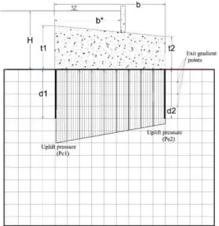
Khosla et al. (1936) used an independent variable technique to develop a method by which seepage characteristics under weirs including different seepage features, such as aprons, floor slopes and a varied number of cut-offs, could be analysed. Khosla’s theory is based on an analytical solution (conformal mapping concept) and experimental data analysis. According to this theory, complex sub-structures related to seepage control variables can be split into three categories: end sheet piles (cut-offs), intermediate cut-offs and depressed floors. By this method, the uplift pressure values could separately be determined at a specific points (key points). Pressure values must be corrected based on the interaction effects between these variables (Garg, 1987; Khosla et al., 1936).
9
(Eq. 2.1). Khosla et al. (1936) recommended that the exit gradient safety factor is: 4 to 5 for gravel, 5 to 6 for coarse sand and 6 to7 for fine sand. The safety factor is the ratio of the critical exit gradient to the computed exit gradient (Delleur, 2006). The exit gradient is computed as given by Eq. (2.1):
𝑖𝑒 = ℎ
𝜋𝑑√𝜆 (2.1)
Where 𝑖𝑒 is the exit gradient by Khosla et al. (1936) theory, h is total head, d is length of
downstream cut-off and 𝜆 is computed by equation 2.2
𝜆 = √1 + 𝛼1
2 + √1 + 𝛼 22
2 (2.2)
Where 𝛼1 =𝑏1
𝑑 , 𝛼2 = 𝑏2
𝑑 as shown in Figure 2.1 and the factor of safety can be computed by F. S = ic
ie , ic=
γsub
γw or ic =
(GS−1)
(1+e) .
Where GS is the specific gravity of the soil, e is void ratio, ic is critical exit gradient, γsub is the submerged soil density, γwis weight water density.
Figure 2.1 One cut-off with apron (Khosla et al., 1936)
10
2.2
Approximate Solutions of Seepage
2.2.1
Fragment Method
Pavlovsky (1935) developed the approximation fragment method to determine seepage characteristics easily and directly under HWRS. In this method, the seepage flow domain was divided into a certain number of fragments. An imaginary section was assumed, where the equipotential line could be considered a vertical line (Harr, 1962). Therefore, flow rate and consequent head could be computed for regular shape regions. The mathematical expression of this theory is expressed below as:
Qm=khm /m (2.3)
Where: m= 1, 2, 3,…, n, Qm= discharge passed through fragment
hm = head loss through fragment
m = dimensionless shape factor depends on the geometry of the fragment
And when discharge for all fragments is the same
Q = kh1/1 = kh2/2 = kh3/3……. Khn /n
Q = k hm/m (2.4)
Q = Khm
∑ =
kh
∑n
m=1 m
(2.5)
Where h without a subscript is total head loss. Therefore, by a similar method:
h =h 𝐦
∑ (2.6)
Consequently, the distribution of pressure head and exit gradient can be estimated as head losses have been computed. Also, there are many standards and forms to calculate the shape factor for each fragment easily according to the geometry and location of these fragments.
11
Recently, many researchers have utilized the fragment method to determine seepage characteristics for the stop during filling in the mining industry (Madanayaka & Sivakugan, 2016; Sivakugan & Rankine, 2011; Sivakugan, Rankine, Lovisa, & Hall, 2013). For these studies, the solutions using fragment method were compared to numerical simulation and the results demonstrated good agreement with the numerical solution.
2.2.2
Flow Net Method
Flow net is one of the easiest and most prominent approximation methods used for seepage analysis. It depends on many sketching trials of equipotential lines and streamlines. These lines must be drawn in such a way that each equipotential line intersects the streamline orthogonally. When an imaginary grid of equipotential line and streamline is created, seepage characteristics can be determined at each intersection point using Eq. (2.7) (Das, 2008; Lambe & Whitman, 1969; Terzaghi, Peck, & Mesri, 1996).
q = Nf△ q = khNf
Nd (2.7)
Where: h = total hydraulic head or difference in elevation of water between upstream and downstream, Nd = number of potential drops, Nf = number of flow channel, k = soil conductivity (L/T), q = discharge (L3/T).
2.3
Analytical
Solution/Conformal
Mapping
by
Schwarz-Christoffel
Transformation
12
𝑑𝑧 𝑑𝑡 =
𝐴
(𝑎 − 𝑡)𝛼⁄𝜋∗ (𝑏 − 𝑡)𝛽⁄𝜋∗ (𝑐 − 𝑡)𝛾⁄𝜋∗ … . (2.8)
Where A refers to a complex number in z-plan and a, b and c are the real constants corresponding to the projection location in z-plane and α, β and γ represent the external angles of the polygon.
A substantial amount of research has been conducted based on this technique. Elganainy (1986) determined the exit gradient and seepage flow for a filter constructed between two hydraulic structures and at the downstream, using a conformal mapping technique. Elganainy (1987) utilized the Schwarz–Christoffel method to derive a mathematical solution (for exit gradient and uplift pressure) for new conditions of Nile barrages and the subside weir. Ilyinsky and Kacimov (1991) demonstrated the procedure to compute the ground water flow around cut-off walls and to trench. The adopted conformal mapping concept conjugated with the variation method. Ilyinsky, Kacimov, and Yakimov (1998) reviewed different techniques, inverse method, variation theorems and optimization process, to develop an analytical solution for seepage under hydraulic structures.
Additionally, conformal mapping method has been used by Farouk and Smith (2000) to derive the exit gradient and potential seepage equations for hydraulic structures with two intermediate filters. Jain (2011) derived mathematical models to determine seepage flow parameters underneath a weir with aprons, two cut-offs, finite depth condition and step at down side. Ijam (2011) used the Schwarz–Chrisoffel transformation method to obtain an analytical solution for seepage flow under hydraulic structures to analyze many variables in the seepage equation, such as cut-off wall with variable locations and angles.
13
approximation and analytical solution for this study is not possible. Hence, numerical method based on the finite element method (FEM) is adopted in developing the linked S-O approach.
2.4
Numerical Solution
The numerical solution is considered more beneficial than analytical and approximation solutions, as complex seepage problems can be solved precisely. Analytical solutions are based on many simplified assumptions, such as isotropic, homogeneous soil properties, which are not always correct. Moreover, the upstream water level is assumed as horizontal level, and the seepage flow domain is mostly considered in a rectangular shape. These assumptions are not necessary for numerical methods. The numerical model can be utilized to solve complex seepage problems, including different boundary conditions. Hence, several efficient numerical methods such as finite difference method (FDM) and FEM are used to solve and simulate a large number of seepage related problems (Wang & Anderson, 1995).
2.4.1
Finite Element Method (FEM)
The FEM is based on the approximation integration approach to solve differential governing Laplace equations (Jain, 2011). FEM solves complex problems with accurate results that is not possible using the closed form solution. The results are more accurate and precise if more time and effort are spent on the computational process (Rao, 2013).
The small panels resulting from subdivision of the flow domain or continuum are called finite elements. Each element is connected with an adjacent element by nodal points (nodes), which lie on the element boundaries. Variation of any design variable or parameter through the continuum is not easy to be determined. Hence, the interpolation model (approximate simple function) is assumed to identify seepage variable values for each node. By applying the interpolation model, boundary condition and governing equation, the variable value for each node can be calculated accurately (Rao, 2013).
The steps of the FEM process are summarized as:
1. Subdividing the continuum of the problem into finite elements with a certain number, size and shape depending on the problem feature.
2. Finding the best interpolation model describing boundary conditions and variables variation. The interpolation model is mostly derived as a simple polynomial (linear, quadratic or cubic).
14 5. Solving the control equation for each node.
In 1970, FEM was applied for the first time by Neuman and Whiterspoon for steady state seepage problems involving anisotropic heterogeneous soil and different boundary conditions. The efficiency and accuracy of the FEM solution compared to experimental, analytical and published results was demonstrated by Neuman and Whiterspoon (Chen, Huan, & Ma, 2006)
As FEM provides precise solutions, numerous researchers have utilized FEM to solve seepage problems. Lefebvre, Lupien, Pare, and Tournier (1981) used FEM to evaluate different scenarios to control and reduce the exit gradient value for embankment dams. Alsenousi and Mohamed (2008) studied the effect of inclined cut-offs for varying distances and angles. Heterogeneous and anisotropic underlying soil layers with limited depth were assumed for the numerical model. Tatone, Donnelly, Protulipac, and Clark (2009) evaluated the efficiency of 21000m2 plastic concrete cut-off in a newly constructed dam in northern Ontario. FEM models were developed to simulate seepage flow of the dam to be compared to drilling investigations and laboratory tests.
Azizi, Salmasi, Abbaspour, and Arvanaghi (2012) utilized hydraulic design data and the structural parameters of a diversion dam to simulate the flow process. SEEP/W based on FEM software was used to evaluate hydraulic design parameters. El-Jumaily and AL-Bakry (2013) utilized the finite volume method to analyze seepage through permeable soil. Furthermore, he studied the effects of anisotropic and non-homogenous soil on uplift pressure and exit gradient.
Mansuri, Salmasi, and Oghati (2014) determined the effects of positions and angles of cut-offs on exit gradient, seepage flow and uplift pressure underneath a diversion dam. Moharrami, Moradi, Bonab, Katebi, and Moharrami (2014) evaluated the effects of cut-off beneath dams to reduce uplift pressure and prevent piping problems. Shahrbanozadeh et al. (2015) adopted a complementary numerical method ISO-geometrical analysis (IGA) and FEM to determine the uplift pressure and exit gradient value for a hydraulic structure model. They compared the experimental results to approximation methods and numerical methods solutions to demonstrate that FEM and IGA provide the most accurate solutions.
15
solution. Therefore, the machine learning technique is utilized to develop surrogate models based on many input and output data sets simulated by the FEM numerical method to accurately predict numerical responses within inked S-O models.
2.4.2
SEEP/W numerical seepage modeling and limited validation
The Geo-Studio SEEP/W software (numerical model) based on FEM was used to find the seepage characteristic value for all simulated seepage scenarios in this study. The seepage characteristics obtained by SEEP/W were solely utilized to create training data (input-output data sets) to train surrogate models, or to evaluate the seepage characteristics of the optimum solution obtained by the S-O technique. SEEP/W can efficiently solve different seepage problems, such as saturated/ unsaturated cases, steady/ transient states, multilayer system and isotropic / anisotropic / heterogeneous hydraulic conductivity, etc. Furthermore, the effect of other geotechnical considerations, stresses, loads, boundary conditions and soil parameters can be combined with SEEP/W numerical seepage simulation. This is achieved based on integrating the provided Geo-Studio components, such as SLOP/W, SIGMA/W and QUAKE/W, with the SEEP/W model (Krahn, 2012). However, it should be noted that the linked simulation-optimization methodology being proposed here is not dependent on a particular simulation model. Indeed, it is possible to easily replace SEEP/W by an even more robust or efficient simulation model in the future. In that case, only surrogate models will require fresh training and validation.
Many researchers have applied SEEP/W for different problems.Chenaf and Chapuis (2007) utilized SEEP/W as a numerical model to validate many approximation equations used to describe a seepage system related to a pumping well. Oh and Vanapalli (2010) combined SLOPE/W and SEEP/W to study the effect of water infiltration on the stability of homogenous compacted embankments. White, Beaven, Powrie, and Knox (2011) used SEEP/W numerical solutions to compare with observed depths of drained liquid resulting from field testing of the leachate recirculation model for different periods. Chapuis, Chenaf, Bussière, Aubertin, and Crespo (2001) conducted a precise validation for SEEP/W solution compared to the analytical solution of different seepage problems.
16
the closed form solution. The mean absolute error (MAE) for the uplift pressure obtained by SEEP/W was 0.905 (2.5%) and for exit gradient was 0.041 (4.6%), as shown in Figures 2.2 and 2.3.
Figure 2.2 Validation of the SEEP/W solutions (uplift pressure)
Figure 2.3 Validation of the SEEP/W solutions (Exit gradient)
2.5
Meta Model (Surrogate Model)
The surrogate models in the linked simulation optimization model have been efficiently utilized to imitate the numerical model responses for complex and computationally expensive problems. Furthermore, meta modeling techniques have been implemented to enhance understanding of input design variable effects on the output design variable. Also, meta models are used as predictors for future expectations of some variables in a specified design. Developing an efficient surrogate (meta) model is based on selecting an adequate machine learning technique and
0.00 20.00 40.00 60.00 80.00 100.00 120.00
1 2 3 4 5 6 7 8 9 10 11 12 13 14 15 16 17 18 19 20 21 22 23 24 25 26 27 28 29 30 31 32 33 34 35 36 37 38
up
lif
tp
ressu
re
(m
)
Uplift pressure by SEEPW
Uplift pressure by closed form solution
0.000 0.500 1.000 1.500 2.000 2.500 3.000 3.500 4.000 4.500 5.000
1 2 3 4 5 6 7 8 9 10 11 12 13 14 15 16 17 18 19 20 21 22 23 24 25 26 27 28 29 30 31 32 33 34 35 36 37 38
Exit
gradein
t
Exit gradient by SEEPW
17
sufficient and uniformly distributed data sets. Many studies have utilized different machine learning techniques to develop efficient surrogate models for hydraulic structures and ground water applications. The most efficient machine learning techniques are artificial neural network (ANN), support vector machine (SVM) and Gaussian process regression (GPR).
2.5.1
Artificial Neural Network (ANN)
ANN imitates human brain neurons, which can change responses according to different environments and / or actions. In the 1940’s, McCulloch and Pitts designed the first neural network, and at the end of this year, Donal Hebb designed the first learning law for ANN. In 1972, Kohonen and Anderson developed strength theory between neurons. Between 1958 and 1988 Rosenblatt, Block, Minsky, Widrow and Hoff submitted a complementary concept for ANN, such as input layer perceptron, connection to associated neurons, fixed weights and other learning rules (Ersayın, 2006; Sivanandam, Sumathi, & Deepa, 2006).
For seepage and ground water problems related to hydraulic structures, ANN has been utilized to simulate and identify seepage characteristics. Garcia and Shigidi (2006) utilized ANN as an approximation model to compute aquifer transmissivity and hydraulic head values. Ersayın (2006) developed an ANN model to predict the phreatic line (seepage path) in an earth fill dam (Jeziorsko Dam) in Poland. Szidarovszky, Coppola, Long, Hall, and Poulton (2007) combined numerical models with the ANN model (hybrid-ANN numerical) to improve the simulation of groundwater characteristics. Kim and Kim (2008) used the ANN method to predict relative crest settlement of concrete faced rock fill dams. Predicted results of the utilized methodology showed good agreement with conventional methods.
Joorabchi, Zhang, and Blumenstein (2009) successfully developed ANN models to simulate and predict the ground water fluctuation based on many variables, such as water table, tide elevation, beach slope and hydraulic conductivity, in five locations on the east coast of Australia. Nourani, Sharghi, and Aminfar (2012) used a single ANN model to predict head values for each piezo-metric on upstream and downstream of different sections of the Sattarkhan earth fill dam (Iran). Santillán, Fraile-Ardanuy, and Toledo (2013) developed an ANN model for seepage analysis beneath a hydraulic structure, considering different water head. Al-Suhaili and Karim (2014) presented a methodology based on the ANN model to optimize the cost of cut-off walls and floors for small hydraulic structures constructed on permeable foundation using genetic algorithm (GA).
18
as Bayesian regularization and Lievenberg-Marquardt, which can be used to decrease overfitting effects. Also, the early stopping and regularization technique significantly improves performance of the ANN model. The early stopping strategy monitors training error and validation error. The training process is continued while training and validation errors decrease. However, when training error decreases and validation error increases (overfitting phenomena), the training process stops too soon (early stopping) and the optimum value of weight and biases are saved. The regularization technique evaluates performance of the ANN model not only based on the error of predicted data, but it tries to minimize the summation of weights and biases to provide smother responses.
2.5.2
Support Vector Machine
Originally, Vapnik (1999) developed and discussed the advantages of using optimal spreading hyper plane in classification and regression machine learning problems. He showed that the generalization ability of the developed technique with fewer support vectors is better. The SVM has the ability to overcome the over-training (overfitting) phenomena (Raghavendra.N & Deka, 2014; Vapnik, 2013). Recently, SVM has been widely used in research in civil engineering and hydraulic structure disciplines (Fisher, Camp, & Krzhizhanovskaya, 2016; Mahani, Shojaee, Salajegheh, & Khatibinia, 2015; Parsaie, Yonesi, & Najafian, 2015; Ranković, Grujović, Divac, & Milivojević, 2014; Su, Chen, & Wen, 2016). Many other researchers have employed SVM for different purposes related to water resources and hydrology application (Azamathulla, Ghani, Chang, Hasan, & Zakaria, 2010; Bhagwat & Maity, 2012; Cimen, 2008; Eslamian, Gohari, Biabanaki, & Malekian, 2008; Goel & Pal, 2009; Han, Chan, & Zhu, 2007; Hipni et al., 2013; Khan & Coulibaly, 2006; Lin, Cheng, & Chau, 2006; Misra, Oommen, Agarwal, Mishra, & Thompson, 2009; Moghaddamnia, Ghafari, Piri, & Han, 2009; Ranković et al., 2014; Samui, 2011; Yu, Chen, & Chang, 2006).
19
The majority of previous studies were implemented in predicting/forecasting responses of a certain variable based on tr