Grid computing and biomolecular simulation

Grid computing and biomolecular simulation

BY CHRISTOPHER J. WOODS1, MUAN HONG NG2, STEVEN JOHNSTON2, STUART E. MURDOCK1,2, BING WU3,4, KAIHSU TAI4, HANS FANGOHR2, PAUL JEFFREYS3, SIMON COX2, JEREMY G. FREY1, MARK S.P. SANSOM4

AND JONATHAN W. ESSEX1 1

School of Chemistry, and2Southampton e-Science Centre, University of Southampton, Southampton, UK

([email protected]) 3

Oxford e-Science Centre, and4Department of Biochemistry, University of Oxford, Oxford, UK

Biomolecular computer simulations are now widely used not only in an academic setting to understand the fundamental role of molecular dynamics on biological function, but also in the industrial context to assist in drug design. In this paper, two applications of Grid computing to this area will be outlined. The first, involving the coupling of distributed computing resources to dedicated Beowulf clusters, is targeted at simulating protein conformational change using the Replica Exchange methodology. In the second, the rationale and design of a database of biomolecular simulation trajectories is described. Both applications illustrate the increasingly important role modern computational methods are playing in the life sciences.

Keywords: Grid; replica exchange; protein conformation; simulation trajectory; storage; analysis

1. Background

Grid computing is becoming increasingly important in the area of the life sciences. Two particular aspects dominate. First, distributed computing is a potentially powerful approach for accessing large amounts of computational power. Cycle stealers, which allow a PC user to donate the spare power of their computer, are now used in a wide range of scientific projects, e.g. the SETI@home study,1 the CAN-DDO cancer screening project2and [email protected] stealers are also becoming more widely used in the pharmaceutical industry, particularly for virtual screening projects. It should be noted that cycle stealers are only one aspect of Grid computing, and that there are many other examples that may be useful in the domain of biomolecular simulations. Second, large databases are used to hold the substantial amount of data now involved in the study of biological systems, and have found particular prominence in the field of bioinformatics. In this paper, two

Published online26 July 2005

One contribution of 27 to a Theme ‘Scientific Grid computing’.

1

http://setiathome.ssl.berkeley.edu.

2_{http://www.chem.ox.ac.uk/curecancer.html.} 3

recent developments in each of these areas, as applied to biologically relevant problems, will be described.

2. Distributed computing

While the use of cycle stealers can provide supercomputer-like resources, their use is limited to calculations that may be split into many independently parallel parts (i.e. coarsely parallel simulations). The distributed and unreliable nature of this resource makes it unsuitable for closely coupled parallel calculations. For these calculations, the speed and latency of inter-processor communication are a bottleneck that cannot be overcome simply through the addition of more nodes. Unfortunately, a large number of chemical simulations require closely coupled parallel calculations, and are thus not suitable for deployment over a distributed computing cluster. An example of such a simulation is the investigation of protein conformational change. These simulations are typically performed using molecular dynamics (MD) (Leach 1996), where the motions of the atoms are integrated over time using Newton’s laws. These simulations cannot be broken up into multiple independent parts, as each nanosecond of MD must be run in series and in sequence.

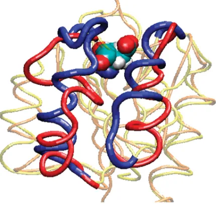
The investigation of protein conformational change is important as it lies at the heart of many biological processes, e.g. cell signalling. Some bacteria regulate nitrogen metabolism using one such signalling pathway. Nitrogen regulatory protein C (NTRC; Peltonet al. 1999) plays a key role in this pathway. Changes in nitrogen concentration activate the kinase NTRB. This phosphorylates an aspartate residue in NTRC, causing it to change conformation (figure 1;Pelton

et al. 1999). This change in conformation allows the NTRC to join together to form oligomers, which then activate the transcription of genes. These genes are used to produce proteins that are used in nitrogen metabolism (Pelton et al. Figure 1. The native (blue) and phosphorylated (red) conformations of NTRC. The site of

1999). A key stage of this pathway is the change in conformation that occurs in NTRC when it is phosphorylated. It is difficult to study this conformational change experimentally via nuclear magnetic resonance (NMR) or X-ray crystallography as the phosphorylated form of NTRC has a very short lifetime of only a few minutes at 258C (Kernet al. 1999). It is thus desirable to model the NTRC protein and encourage the conformational change by simulation.

(a) The replica exchange method

We can use a distributed computing cluster to investigate protein conformation-al change via Replica Exchange simulations (Hansmann 1997;Sugitaet al. 2000). Multiple replicas of the protein are run in parallel, each running under a different condition, e.g. temperature. Periodically the potential energies of a pair of replicas running at neighbouring temperatures are tested according to a replica exchange Monte Carlo test (Hansmann 1997;Sugitaet al. 2000) and, if the test is passed, the

coordinates of the pair of replicas are swapped. This enables simulations at high temperatures, where there is rapid conformational change, to rain down to biologically relevant temperatures where conformational change occurs more slowly. The testing of neighbouring temperatures introduces a light coupling to the simulation, meaning that it no longer fits the archetypal coarsely parallel distributed computing model. This light coupling introduces inefficiencies to the scheduling of the simulation, as any delay in the calculation of one temperature can propagate out to delay the calculation of all temperatures. To help overcome this, a catchup cluster has been developed that monitors the simulation for temperatures that are taking too long to complete, and that are likely to negatively impact the overall efficiency of the simulation. Once identified, the calculation of these temperatures is rescheduled onto a small, yet fast and dedicated, computational resource so that they can ‘catchup’ with the other temperatures (figure 2). The scheduler identifies which replicas should be moved to the catchup cluster by scanning the replicas and seeing if any is waiting for their partner to complete the current iteration. If a replica has been waiting for more than 10 min, then an estimate is made of how much progress the partner has made, based on how long it has been running, and the average completion time of an iteration based on the average of the times collected up to that point. If the partner has completed less than 10% of the iteration, then it is moved onto the catchup cluster. This algorithm was necessary as the catchup cluster was a limited resource and was able to catchup only two replicas at a time. By concentrating on the replicas that were less than 10% complete, it was possible to focus the use of the catchup cluster on the replicas that most needed it. The figure of 10% was arrived at through initial experimentation that monitored the number of replicas that were passed to the catchup cluster, ensuring that the catchup cluster was neither over-used, thus leading to replicas waiting in the catchup cluster queue, or under-used, leading to idle resources.

3. Experimental details

NMR structures of the phosphorylated (1DC8) and unphosphorylated (1DC7) conformations of the NTRC protein were obtained from the protein databank.4 Polar hydrogen atoms were added via WhatIf (Vriend et al. 1997). The proteins were solvated in 603A˚3 boxes of TIP3P water and sodium ions were added via the XLEAP module of AMBER 7.0 (Pearlman et al. 1995) to neutralize the system. The CHARMM27 force field (Mackerrell et al. 1998) was used, and the systems minimized, then annealed from 100 to 300 K. The systems were finally equilibrated for 100 ps at constant temperature (300 K) and pressure (1 atm). The final structures from equilibration were used as the starting structures for all of the replicas.

The temperatures for each replica were chosen using a custom program that optimized the temperature distribution such that a replica exchange move was accepted with a probability of 20%. This resulted in a near uniform distribution of temperatures, ranging from several replicas below the target temperature of 300 K (290.1 K) to a maximum of 400 K. In total 64 replicas were used for each of the two proteins. As the lowest and highest temperature replicas attempt exchange moves at half the rate of the other replicas, it is common practice to add additional replicas 4

below the target temperature. Replicas may thereby swap into the target temperature from both lower and higher temperature simulations. The choice of a 20% acceptance probability was made to minimize the number of replicas required for simulation, i.e. the computational expense, while still allowing sufficient exchange moves to be accepted for the replicas to move in temperature. Further information regarding common practice in replica exchange simulations of explicitly solvated proteins may be found elsewhere (Wiley 2004).

The simulations were conducted using NAMD 2.5 (Kaleet al. 1999). A replica exchange move was attempted between neighbouring temperatures every 2 ps, after the initial 20 ps of sampling that was used to equilibrate each replica to its initial temperature. A Langevin thermostat (Paterlini and Ferguson 1998) and a Nose–Hoover Langevin piston barostat (Felleret al. 1995) were used to sample at constant temperature and pressure, while SHAKE (Ryckaert et al. 1977) was used to constrain hydrogen bond lengths to equilibrium values. A 1 fs time step was used for the MD integrator, and the non-bonded interactions were evaluated using a 12 A˚ cut-off and the particle mesh Ewald sum (Dardenet al. 1993).

(a) Details of the distributed cluster

The simulations were run over the Condor (Litzkow 1987;Litzkowet al. 1988) cluster provided by the University of Southampton. This cluster uses Condor (Litzkow 1987; Litzkow et al. 1988) to make available the spare cycles of approximately 450 desktop computers running Microsoft Windows NT 5.1 at different locations within the University of Southampton. The two replica exchange simulations were run simultaneously on this cluster. There was little competition between the two simulations for nodes as they each required a maximum of 64 nodes out of the available 450.

This Condor cluster was chosen as, for our purposes, it was a good model for a computational Grid. The Condor cluster provided a distributed, heterogeneous resource of processors that were geographically diverse, managed via different groups, and connected via networks of varying quality. The problems that we experienced running on this resource were, we believe, typical of those that we would have experienced if we were using an actual distributed computing Grid. By running on only Southampton machines, we were able to get a guarantee of service with regards to network speed, security and support that, at the time, we did not believe we could attain from a truly Grid resource. It should be possible to run these replica exchange simulations over a Grid resource using a Grid scheduler such as Condor-G.5

(b) Implementation of the catchup cluster

The catchup cluster was implemented via dedicated dual Xeon 2.8 GHz nodes running Linux. Each Xeon processor was able to provide two virtual processors, allowing NAMD to run in parallel over four virtual processors per node. The fast catchup cluster consisted of two dual Xeon nodes, thus allowing it to catchup two replicas simultaneously.

To test the utility of the catchup cluster, it was only made available to the replica exchange simulation on the phosphorylated conformation of the protein (1DC8). 5

As both replica exchange simulations were running simultaneously, any differences in efficiency should thus be wholly attributable to use of the catchup cluster.

4. Results

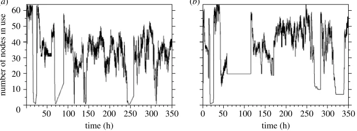
Figure 3 shows the number of nodes in use during the replica exchange simulations on the phosphorylated and unphosphorylated conformations of NTRC. The initial phase of the simulation involved the 20 ps of equilibration of each replica to its initial temperature. This was broken down into 10 iterations of 2 ps. As there were no replica exchange moves during these first 10 iterations the replicas were all independent and thus the maximum number of 64 nodes were in use. However, there were efficiency problems during this phase of the simulation, as the unreliable nature of the distributed cluster caused several short periods of downtime that stopped both simulations. Frequent periods of downtime were common throughout the rest of replica exchange simulations.

The second stage of the simulations occurred when the replicas begun to complete their 10th iteration. At this point each replica had to wait for its partner to complete 10 iterations such that the pair of replicas could be tested and potentially swapped. Owing to the range of processors available in the distributed cluster and the different impact of downtime on each of the replicas, there was a large spread of times over which each replica completed 10 iterations. This meant that a large number of replicas were left waiting for a significant time for their partner to complete, and thus the number of nodes in use for each simulation dropped from the maximum of 64 down to approximately 30. If the efficiency is defined as the ratio of the number of nodes in use compared to the theoretical maximum, then the efficiency dropped from 100% down to about 47%.

After this dip in efficiency, the simulations then moved towards the final stage, which was a steady state, where the number of replicas running and the number of replicas waiting for their partner to complete reached a consistent range of values. This steady state was periodically disrupted by failure of the condor cluster, but was always quickly recovered once the disruption was over. The steady state for the simulation that used the catchup cluster had significantly

60

50

40

30

20

10

0 _{50 100 150 200 250 300 350}

time (h)

50

0 100 150 200 250 300 350

time (h)

number of nodes in use

(a) (b)

more replicas running, and significantly fewer replicas waiting compared to the simulation that did not use the catchup cluster. The catchup cluster clearly improved the steady state number of nodes in use to approximately 50, compared to approximately 40 for the simulation that did not use the catchup cluster. This is an improvement in efficiency from 63 to 78%.

(a) The heterogeneous distributed cluster

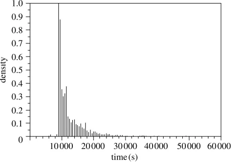
The distributed condor cluster consisted of a range of desktop computers with varying processor speeds. To investigate the effect of running the simulation on this heterogeneous cluster, the total simulation time for each iteration was histogrammed. The histogram of replica completion times for the phosphorylated form of the protein is shown infigure 4. This figure shows that while the majority of iterations completed in under 10 000 s (2.8 h), there was a significant spread of replica completion times up to 20 000 s (5.6 h). This spread of completion times caused problems for the scheduling of the simulation as it meant that pairs of replicas that started at the same time could finish at very different times. This meant that as the scheduler had to wait for both replicas to finish, the simulation was effectively slowed down to the speed of the slowest nodes.

(b) Comparison to normal MD

The use of dual Xeons in the catchup cluster aiding the efficiency of a replica exchange simulation was compared to their use as dedicated nodes running a normal MD simulation. The phosphorylated conformation of NTRC was simulated at 300 K using a standard MD simulation with an identical starting structure as the replica exchange simulation and identical simulation conditions. Over the same period of time as the replica exchange simulations were running, this MD simulation on a single dual Xeon node completed 1.9 ns of dynamics. This compares to a total of 10.5 ns of dynamics generated by the corresponding replica exchange simulation. However, the 1.9 ns of dynamics generated via the MD simulation forms a single, self-consistent trajectory. In comparison, the

1.0

0.9 0.8 0.7

0.6 0.5

0.4 0.3

0.2 0.1

0

10000 20000 30000 40000 50000

time(s)

60000

density

10.5 ns of sampling from the replica exchange simulations was formed over 64 individual trajectories of only 0.16 ns in length. The dedicated node has produced a single trajectory over 10 times the length of those produced via the distributed condor cluster with catchup cluster. This is despite the dedicated node only running the MD approximately 3.5 times the speed of a typical node in the distributed cluster. There are two reasons for this discrepancy; first, as demonstrated in figure 4, the heterogeneous nature of the distributed cluster meant that there was a large spread in the amount of time needed to complete each iteration of the replica exchange simulation. This could be mitigated against by running each iteration twice at the same time on the distributed cluster and using the results from the first node that completed the calculation. The second reason for the discrepancy is that the distributed cluster was very unreliable, leading to large periods of time when the simulation was not running. This unreliability was both across the whole cluster, when the central manager failed causing the entire resource to fail, and also on individual nodes, on which calculations were regularly interrupted by reboots or user intervention. Unfortunately, the implementation of Condor used for these simulations was not able to migrate a calculation between nodes, meaning that the calculation had to be restarted each time it was interrupted. The replica exchange simulations presented here were run at a time when the condor cluster was experiencing a higher than normal amount of downtime. It is anticipated that during normal operation the condor cluster would be more reliable, and that the steady state efficiency of the replica exchange simulations would be maintained throughout the majority of the simulation. However, the experience of running these simulations demonstrates that applications that use distributed clusters need to include estimates of downtime and the range of available resources when predicting how long a particular simulation will take to run. These results also demonstrate that a distributed computing resource is, unsurprisingly, not efficient compared to a dedicated computing resource. However, distributed computing typically provides resources that would otherwise not be available.

(c) Effectiveness of replica exchange

achievable in months on a dedicated Beowulf cluster composed of 64 dual-Xeon nodes of the type used here for the catchup cluster, would, based on current progress, take over a year on the condor cluster.

5. Summary: distributed computing

Distributed computing provides a resource that is not ideally suited to a wide range of chemistry problems. The investigation of protein conformational change is one such problem. The replica exchange algorithm was used in an attempt to fit this chemistry problem to the distributed computing resource. The coupled nature of replica exchange simulations caused problems for the scheduling of the computation that were partially solved through the development of a dedicated catchup cluster. This cluster improved the efficiency of the replica exchange simulation from 63 to 78%.

6. BioSimGrid: a database for biomolecular simulation

As evidenced by the preceding example, computer simulations play a vital role in biochemical research. These simulations are computationally demanding and they produce huge amounts of data (up to approximately 10 GB each) that is analysed by a variety of methods in order to obtain biochemical properties. Generally, these data are stored at the laboratory where they have been computed in a proprietary format that is unique to the simulation code that has been used. This constrains the sharing of data and results within the biochemistry community: (i) the different simulation results are usually not available to other groups and (ii) even if they are exchanged, for example via FTP, then the data can generally not be compared easily with post-processing tools due to the varying data formats. BioSimGrid will facilitate the comparative analysis of these simulations, allowing more general structure/dynamics/func-tion relastructure/dynamics/func-tionships to be discovered.

BioSimGrid6(Wuet al. 2003;Taiet al. 2004) seeks to tackle this problem by enabling biochemists to deposit their simulation data of varying formats to a shared repository. This will allow biochemists to retrieve a slice or part of a protein in a uniform way for post-simulation analysis. BioSimGrid also provides an integrated analysis environment. By providing a uniform data storage and data retrieval mechanism, different proteins can be compared easily.

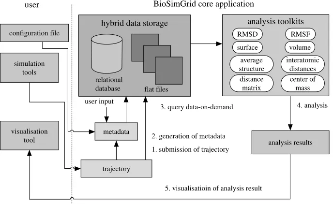
Figure 6demonstrates typical scenarios of using the BioSimGrid project. The completion of a biomolecular simulation delivers simulation data, which is called a ‘trajectory’. A trajectory consists of many frames (corresponding to time steps in the simulation process) of simulation data recording the positions and velocities of all atoms. The first step is to submit the new trajectory and all the relevant meta-data (which describes the simulation and will allow sophisticated querying of all submitted trajectories) to the database. The extraction of the meta-data (from the simulation configuration files) and the trajectories (from the simulation data files) is fully automated, but the user has the option to provide 6

additional information, such as publication references that cannot be extracted from the simulation configuration and data files.

Once the data are stored in the database, users can query different slices of one or more trajectories and perform a number of standard analysis computations (a selection is shown in the figure) on these data. The work flow is then completed by the graphical display of the analysis results (either as vector

hybrid data storage

BioSimGrid core application

relational

database flat files

user input

metadata

trajectory

3. query data-on-demand

2. generation of metadata

5. visualisatioin of analysis result

analysis results 4. analysis

RMSD RMSF

surface volume

average structure

interatomic distances center of mass distance

matrix

analysis toolkits

1. submission of trajectory user

configuration file

simulation tools

visualisation tool

Figure 6. Schematic of the work flow in the BioSimGrid project.

graphics, bitmaps, movies or using interactive three-dimensional environments such as visual molecular dynamics (Dalke et al. 1996) and PyMol (DeLano 2002)). The results are, of course, also available in text or data files.

The following section of the paper discusses two related projects on grid-enabled data storage. Section 8 describes the architecture of BioSimGrid where the data storage layer, the middleware layer and the user interface layer are discussed in detail. Section 9 gives a brief outline on the current issues and the future work on the next prototype, and we finally conclude in §10.

7. Related work

(a) GridPP and the European DataGrid project

GridPP7 is a collaboration project between particle physicists and computer scientist from the UK and CERN aiming to build a Grid for particle physics. One of the key components of GridPP is the European DataGrid Project (EDG)8 which deals with managing a large quantity of sharable data reliably, efficiently and scalably. EDG aims at enabling access to geographically distributed computing and storage facilities. It provides resources to process huge amounts of data from three disciplines: High energy physics, biology and earth observation. EDG has a file replication service to optimize data access by storing multiple copies of local data at several locations. This replication framework has an optimization component to minimize file access by pointing access requests to appropriate replicas and proactively replicating frequently used files based on access statistics.

As compared to DataGrid, BioSimGrid aims to provide a mechanism of data access at a finer granularity level, by delivering a slice of a trajectory rather than a whole file. Hence the concept of file replication of DataGrid can potentially be adopted and modified to suit a finer granularity level of data access.

8. The architecture of BioSimGrid

BioSimGrid seeks to fulfil the following criteria in its implementation:

(i) to minimize data storage, in order to store as many trajectories as possible in a fixed amount of storage space;

(ii) to maximize data transfer rate, in terms of the speed of delivering data to the computational elements, in this case the post-processing tools; (iii) to provide an abstraction of the data layer, where biochemists are freed

from the complication of using and understanding data querying languages and the data storage structure in their scientific research; (iv) to provide a transparency of data location to the users, where actual

physical location of the data is hidden.

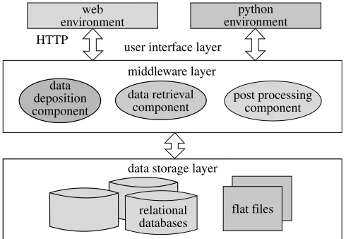
As shown infigure 7, the architecture of BioSimGrid encompasses three layers: the data storage layer, the middleware and the user interface layer. Each of these will be described in the following sections.

7

http://www.gridpp.ac.uk.

8

(a) BioSimGrid data storage layer

The data storage layer is responsible for managing the data on a single machine and exposes methods that are used by the data retrieval component to provide the user with data. This layer is required on each machine that is storing trajectory data, initially there will be six remote sites each running this layer. It provides an API that abstracts from the method used to store the data and provides simple access methods for both querying and retrieving data. The trajectory data is divided into two key sections, the metadata and the coordinate data.

(i) Trajectory metadata

The metadata is additional information about the trajectory that can either be supplied by the user, the input files or calculated at a later stage. It also includes the topology that describes the structure of the protein (chains and residues). This metadata is comparatively small and can be replicated across all sites using standard database replication tools. The advantage of replicating the metadata across all sites is so that a user can query all the trajectories stored in the system by querying a single machine and expect a timely response. This design also helps with scalability and load balancing: since the volume of metadata is small, additional nodes can be added to the system and easily incorporated by simply replicating the database. Since each node stores the topology of all the trajectories, users can use any node to query and process data helping to balance the load across the system.

(ii) Trajectory coordinate data

The coordinates for every atom for every time step are stored resulting in a large volume of data which has to be managed. We have devised a fast, efficient way to store the coordinates using flat files that reduces the storage requirements as well as improving performance results. This flat file method was implemented

web environment

data deposition component

data retrieval component

post processing component HTTP

user interface layer

data storage layer

relational databases

flat files middleware layer

python environment

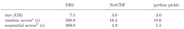
using Python pickle (Drake 1995) and it was compared with a commercial database (DB2) as well as an existing flat file method (NetCDF9). The performance results are shown in table 1. These results show that a flat file method is well suited to our application for both random and serial data access. We selected our own method for flexibility as a whole trajectory is broken into a set of files that are then replicated to at least one other node. This helps to load balance the coordinate data requests as well as provides offsite backups of the data. This abstraction layer also permits the use of different storage methods that can include compression and custom formats, which are completely transparent to the user.

Currently only the coordinates are stored using this method but the next version will store both coordinates as well as velocities.

(b) BioSimGrid middleware

The middleware of BioSimGrid is implemented on a modular architecture to enable easy extension and future plug in. It is written in Python (Drake 1995), a free, open-source and platform-independent high-level object-oriented program-ming language. Python is chosen for several reasons: (i) the biomolecular simulation community are moving towards Python as the preferred environment for post-processing analysis and several mature post-processing tools written in Python exist already (for example, MMTK10 and PyMOL DeLano 2002). (ii) Python can easily integrate and interface to compiled codes so that other existing tools (typically written in FORTRAN or C) can be re-used immediately. (iii) Python comes with a substantial set of standard libraries that can be used in this project and avoid recoding common tasks.

(i) Data deposition component

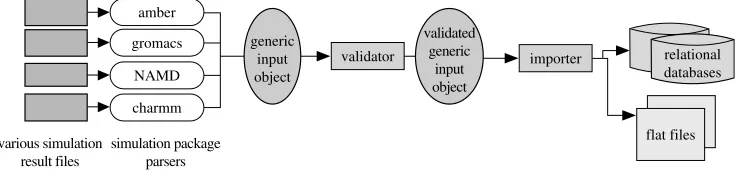
The process of depositing a trajectory into the BioSimGrid database is completely automated and the complication of the underlying storage structure is abstracted from the users. One of the challenges is to cater for different simulation packages that produce simulation data in various file formats. To deal with this, the deposition component consists of different parsers for different simulation packages to parse the simulation data files into a generic input object.

Table 1.Summary of performance results comparing different flat file methods with a commercial database (DB2)

DB2 NetCDF python pickle

size (GB) 7.5 3.0 3.0

random accessa(s) 560.8 16.4 18.6

sequential accessb(s) 389.0 4.9 5.5

a

A random frame is chosen and then read from a trajectory of 1000 frames. This is completed 1000 times with a different frame chosen each time.

b

The same trajectory of 1000 frames is read frame by frame from start to finish.

9

http://my.unidata.ucar.edu/content/software/netcdf/index.html.

10

This object is then parsed through a validator to check for correct data type and their validity against various dictionaries (e.g. the existence of a residue in the dictionary). The process is completed when the validated generic input object is deposited into the flat files (coordinates and velocities) and database (metadata) through an importer. With the modular approach as shown in figure 8, new parsers can easily be added for any new simulation package if required. The underlying complexity of parsing, validating and importing a trajectory into the database is hidden from the users. A biochemist needs only to run five lines of code to deposit their trajectories by specifying the path to their simulation data files, as shown in figure 9.

For the next prototype, the data deposition component will be extended to cater for the distributed nature of the application. We envisage an implementation of multiple deposition points to avoid single point failure and performance bottlenecks. In this case, a global identifier will be assigned to uniquely identify a trajectory and facilitate the synchronization of multiple metadata databases. To deposit a trajectory from a remote location the generic input object will be serialized at the deposition client and deserialized at the deposition server.

(ii) Data retrieval component

The data retrieval component provides a single point of entry for all the trajectories stored on any of the sites. Each site will be running a data retrieval component and a user can use any site to query the data in the entire system. This component queries the local database to retrieve any metadata that is requested, so the user can query information about a trajectory on a different site

various simulation result files

simulation package parsers amber

gromacs

NAMD

charmm

generic input object

validated generic

input object

importer relational databases

flat files validator

Figure 8. The modular implementation of a data deposition component that includes a set of parsers, a validator and an importer. New parsers can be easily added to this modularized component.

from bioSim.Settings import UserSettings

from bioSim.Deposit.NAMDDeposit import NAMDDeposit filenames = {‘parameters’:’/path/paraFile’,

‘topology’:’/path/topoFile’, ‘coordinates’:[’/path/coordFile’] }

uSettings=UserSettings.UserSettings(“guest”) NAMDDeposit.NAMDDeposit(uSettings,filenames)

without having the overhead of contacting the hosting site. This component abstracts the location of the trajectory data from the user and is responsible for getting coordinates from external sites if they are not stored locally.

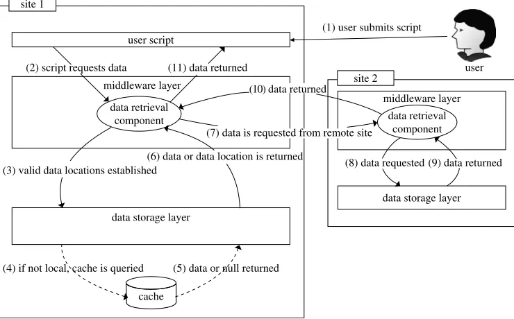
Figure 10shows how the data are transparently retrieved from a remote site so that it can be used by a user’s script. In step 1 and 2 the user submits a script that requests for a set of coordinates from the data retrieval component. This component first looks at the metadata database to retrieve the locations of the requested coordinate flat files (step 3). If the data are stored locally then it is returned otherwise a list of remote data source locations are returned to the data retrieval component (step 6). A data source is then selected from the list and a request is made to the data retrieval component on the remote site for the required data (step 7). As this source is listed as a valid data source it is guaranteed to store the data locally, hence it will not attempt to retrieve the data from another remote site. The data are then passed back to the requesting site (step 10) and the data retrieval component returns the data to the user script (step 11) in the same way as a locally stored data set.

There are two key opportunities to save retrieval times when retrieving large amounts of data. The first is to look at the list of sites that store the trajectory and ask multiple sites to provide different parts of the trajectory. This will reduce the load on sites by distributing it across multiple sites as well as improving the speed that data are received.

The second is a cache (not implemented in the current prototype). Each frame that is retrieved from an external site will be stored using the same flat file storage method. If a whole trajectory is then cached it can be moved to the main database and marked as a valid location to retrieve data for that trajectory.

site 1

user script

(2) script requests data (11) data returned

(1) user submits script

user site 2

middleware layer

data retrieval component

(8) data requested (9) data returned

data storage layer (6) data or data location is returned

(3) valid data locations established

data storage layer

(4) if not local, cache is queried (5) data or null returned

cache middleware layer

data retrieval component

(7) data is requested from remote site (10) data returned

So when a data query requires data that is not stored on the database then the cache is consulted first to see if it has been retrieved previously (step 4 and 5 in 10) if not then the hosting site is queried. There is a limit to the number of frames that are held in the cache and this is defined by a site-specific limit, which also includes the whole trajectories that are added to the local data store. The aim of storing whole trajectories on additional sites is to attempt to move the data closer to the processing. If a site continually requests a trajectory it makes sense to store the trajectory on that site.

Currently each site has an excess of storage space and we can utilize this space to gain a performance boost. However, more trajectories can still be added as temporary trajectories can simply be deleted and removed from the metadata database to make more room as required.

The data retrieval component is not only responsible for getting the data from the distributed sources but it is also responsible for making the data transparently available to the users in an environment of their choice, in this case Python. This result in Python numeric arrays being made available to users who have no idea where or how the data are stored. This has currently been implemented and a series of analysis tools for the post-processing component have been built on this design. This design also permits extensions for other languages like Perl to assist the users to migrate and utilize the BioSimGrid project.

(iii) Post-processing component

For the post-processing component, a set of analysis tools are written for standard and generic analysis on the simulation data, e.g. the calculation of root mean square derivation (RMSD) and the computation of the average structure and interatomic distances. Each analysis is exposed as a module and the modularity approach enables the tool set to be extended easily. An example of an analysis script is shown in figure 11 to demonstrate how to use the post-processing tools. The fourth line of the script initializes the user settings. The fifth line specifies the setting for a frame collection—the part of the protein to be used to perform the analysis, in this case frames 100–200 from trajectory ‘BioSimGrid_GB-STH_1’. The seventh line requests a RMSD analysis by taking the frame collection as its input parameter. Finally, the last line specifies the format of the result to be generated, which in this case is the output of an image file in PNG format. The ease of selecting different data set and different post-processing tools allows biochemists with little computational

from bioSim.DataRetrieval import FrameCollection, FCSettings from bioSim.Analysis import RMSD

from bioSim.Settings import UserSettings u = UserSettings.UserSettings(‘guest’)

f = FCSettings.FCSettings(u,[[‘BioSimGrid_GB-STH_1’,range(100,201)]]) fc = FrameCollection.FrameCollection(f)

myRMSD = RMSD(fc) myRMSD.createPNG()

experience to perform an analysis on the simulation data and obtain meaningful results.

(c) User interface layer

The BioSimGrid user application level offers two modes of interaction: via a graphical web based interface or via the Python scripting environment. The graphical interface is just another layer on top of the underlying Python codes. The scripting environment caters for advanced users who would like to connect to BioSimGrid in a scripting environment and utilize its data submission, retrieval and post-processing API in a fully programmable way. In this environment, biochemists can choose to run existing analysis toolkits provided by BioSimGrid. Alternatively, for more specific analysis, they can use the available data retrieval packages to write their own script. The graphical interface provides a more user-friendly environment to cater for novice users. It allows users to perform standard analysis runs and provides an overview of the available data and processing options. In this mode, a user first selects an analysis from a drop down menu then proceeds to select a trajectory and the relevant frames on which to perform the analysis. All these operations are done by clicks of buttons on a web browser.

9. Current issues and next prototype

BioSimGrid is in its early stage of development. Current prototypes that have been developed are based on architecture where both the application and database server are implemented as client server architecture, running at a single location. We have modularized our components and have developed a basic set of functionalities of BioSimGrid for data deposition, data retrieval and analysis of post simulation data. The modularity approach of the components enables easy plug-in and future extension of various functionalities, such as adding more analysis tools or extending the data deposition tools to cater for new simulation result formats.

The next prototype of BioSimGrid will concentrate on tackling the geographically distributed databases and applications. Establishing secure asynchronous network communication, handling data latency and data recovery is non-trivial in this case. We are investigating Python twisted framework11 and Pyro12 for programming network services and applications. For a more reliable data transmission, the next prototype will incorporate MD513 hashes to help manage corruptions in file transfer. We also envisage the use of standard protocols such as secure socket layer (openSSL) to provide secure point to point communication.

The issue of security is also a major concern in BioSimGrid. We envisage the use of digital certificate-based authentication to authorize users into the system and provide mechanism to set various permission levels for different user groups to authorize them to different resources and transactions.

11_{http://www.twistedmatrix.com.} 12

http://pyro.sourceforge.net/index.html.

13

In the future work, we plan to implement web service based interfaces in order to provide a platform and language independent way of accessing the existing middleware components.

10. Summary: BioSimGrid

In summary, BioSimGrid provides a trajectory storage system that allows users to submit simulation data from a wide range of simulation packages and to run cross simulation comparisons independent of the source of the data. We have developed the current version of the system together with biochemists who provide constant feedback on the usability of the project, and we are currently expanding the user base and the number of available trajectories in the system.

11. Conclusion

Advanced computational methods and Grid computing are finding increasing use in the area of the life sciences. In the particular context of biomolecular computer simulations, we have extended the basic distributed computing model to the situation where the calculations are coupled, through the addition of a dedicated Beowulf cluster to catchup on delayed simulations. This approach does yield an improvement in the overall simulation efficiency. We have also reported the development of a database for the storage and analysis of the large trajectories produced by these simulations. This database will not only allow for extensive and valuable comparisons to be made between related simulations, thereby yielding more a more reliable biochemical interpretation, but will also allow data to be readily shared between laboratories.

For the work on distributed computing, we thank R. Gledhill, A. Wiley and L. Fenu for discussions and the EPSRC for funding comb-e-chem. For BioSimGrid, we would like to thank our collaborators D. Moss, C. Laughton, L. Caves, O. Smart and A. Mulholland. This project is funded by BBSRC.

References

Dalke, A., Humphrey, W. & Schulten, K. 1996J. Mol. Graph.14, 33. Darden, T., York, D. & Pedersen, L. 1993J. Chem. Phys.98, 10 089.

DeLano, W. L. 2002 The PyMOL molecular graphics system.DeLano Sci. (www.pymol.org) Drake Jr, F. L., van Rossum, G. 1995 Python library reference. Computer Science Department of

Algorithmics and Architecture, CS-R9524.http://www.python.org.

Feller, S. E., Zhang, Y. H., Pastor, R. W. & Brooks, B. R. 1995J. Chem. Phys.103, 4613. Hansmann, U. H. E. 1997Chem. Phys. Lett.281, 140.

Kale, L.et al. 1999J. Comp. Phys.151, 283. NAMD was developed by the Theoretical Biophysics Group in the Beckman Institute at Urbana-Champaign.

Kern, D., Volkman, B. F., Luginbuhl, P., Nohaile, M. J., Kustu, S. & Wemmer, D. E. 1999Nature 402, 894.

Leach, A. R. 1996Molecular modelling, principals and applications. Harlow: Longman.

Litzkow, M. 1987 Turning Idle Workstations into Cycle Servers. InUsenix Summer Conference, Litzkow, pp. 381–384.

Mackerrell, A. D.et al. 1998J. Phys. Chem. B.102, 3586. Paterlini, M. G. & Ferguson, D. M. 1998Chem. Phys.236, 243.

Pearlman, D. A., Case, D. A., Caldwell, J. W., Ross, W. S., Cheatham, T. E., Debolt, S., Ferguson, D., Seibel, G. & Kollman, P. 1995Comput. Phys. Commun.91, 1.

Pelton, J. G., Kustu, S. & Wemmer, D. E. 1999J. Mol. Biol.292, 1095. Ryckaert, J. P., Ciccotti, G. & Berendsen, J. C. 1977J. Comput. Phys.23, 327. Sugita, Y., Kitao, A. & Okamoto, Y. 2000J. Chem. Phys.113, 6042–6051. Tai, K.et al. 2004Org. Biomol. Chem.2, 3219. (doi:10.1039/b411352g.) Vriend, G., Hooft, R. W. W. & Van Aalten, D. 1997WhatIf.

Wiley, A. P. 2004 The computational investigation of conformational change Ph.D. thesis, University of Southampton.