Mapping Queensland land cover according to FAO LCCS using multi-source spatial data

2. CONSTRUCTING THE CLASSIFICATION SCHEME

Earth surface mapping was given a tremendous boom with the introduction of earth observation satellites in 1972. Land cover and land use maps at various scales were generated to address specific needs or local areas, but none of the classification schemes became internationally recognized or standardized. Under this context, the Land cover classification system (LCCS) adopted by the FAO can be considered as an approach with logical definitions which apply all land cover types of the world (Di Gregorio and Jansen, 2000). FAO and UNEP gathered in 1993 to establish a land cover classification system to match the wider spectrum of global land cover types and so by 2000 the FAO LCCS became fully operational.

2.1 Basics considered in FAO LCCS

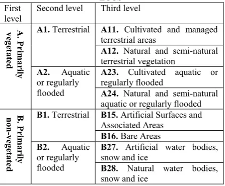
The FAO LCCS system is consider as the only such approach available today which can be applied to any region of the world regardless of the economic conditions and data source. Initially, the FAO method is a “priori” classification system, which defines all the classes before the classification is conducted. The advantage of this approach is the possibility to maintain standardisation of classes. For this propose, LCCS developed pre-defined classification criteria, or classifier to identify each class, instead of identifying the class itself. This concept is based on the idea that a land cover class can be defined without considering its location or its type, using a set of pre-selected classifiers. Therefore, when the user requires a large number of classes, a large number of classifiers are required. To organize the classification more easily, FAO system used a dichotomous (divide into sub categories), approach in hierarchical levels and used eight classifiers to group all land cover types at the third level. In other words, any location on the earth surface can be categorized into one of the eight classes without having a conflict. Up to this third level, FAO used the presence of vegetation, edaphic (plant conditions generated by soil and not by climate), and artificiality of land cover for classification. Additionally, the third level of FAO classification can be considered as a concept based on visual classification, which uses the directly visible and knowledge based components on the ground.

In practical conditions, a further breakdown of the third level eight classes must be conducted to obtain a detailed level of land cover classes. For that purpose, FAO uses a hierarchical approach, or the Modular-Hierarchical Phase, to build additional classifiers, but strictly within one of eight classes identified in third level of the dichotomous phase. Under this 4th phase, the system uses a set of pre-defined pure land cover classifiers, different from the eight classes in the dichotomous phase presented in Table 02.

Table 02. Dichotomous approach to build primary classes in FAO LCCS

First level

Second level Third level

A. Prim a r il y v e g e ta ted

A1. Terrestrial A11. Cultivated and managed terrestrial areas

A12. Natural and semi-natural terrestrial vegetation

A2. Aquatic or regularly flooded

A23. Cultivated aquatic or regularly flooded

A24. Natural and semi-natural aquatic or regularly flooded

B. Prim a r ily non -v e g e ta ted

B1. Terrestrial B15. Artificial Surfaces and Associated Areas

B16. Bare Areas B2. Aquatic

or regularly flooded

B27. Artificial water bodies, snow and ice

B28. Natural water bodies, snow and ice

The pure land cover classifiers are defined by Environmental Attributes (e.g., climate, soil, and etc) or by Specific Technical Attributes (specific details like crop type and soil type) (africover, 2008). In both cases, the user gets the freedom to add these classifiers with their own research interests, scale of the classification, and the physical and climatological conditions of the field. The FAO LCCS document presents a large number of classifiers to use in this level and the user can use only a selected set from the list to match with the scope of their own mapping project.

2.2 Australian vegetation and its recent changes

The Australian flora and fauna is a composite of Gondwanan elements, and has evolutionary lines shared with South America. About 80% of the flora of Australia is endemic to the country and most of the species are extremely restricted in geographic and climatic range. For example, 53% of the about 800 species of eucalypts have climatic ranges spanning less than 3˚C mean annual temperature, and 25% span less than 1˚C (Hughes, 2005). Also, about 23% have adapted to less than 20% of mean annual rainfall changes (Barrie, 2003). The recent global warming may have influenced these flora (and fauna), since the largely flat Australian geography offers only a little space to escape naturally.

The millions of years old unique Australian landscape has faced a rapid change within last two centuries with the arrival of European settlers. The native vegetation cover or plants present in Australia before European settlement has declined to 87% of the country (State of Environment, 2006). Most of the native forest change has occurred through clearing of forests and woodlands, which originally covered 54% of the country and now covers only 42%. Within this period, an excessive loss occurred in rainforest and vine thickets, eucalyptus woodland, Mellee woodlands, and low closed forest categories by over 30%. According to overall assessments, about 22% of the forest and woodland have been lost due to burning and farming by settlers (State of Environment, 2006). These recent manmade and other climatic influences on the land surface have attracted the attention of researchers.

2.3 Applicability of FAO LCCS system in Australian terrain

Australian land cover is greatly influence by climate rather than it’s near flat terrain with 99% of its land area below 1000m (Hughes 2003). Figure 1 compares the annual rainfall and topography of the country, which shows heavy rainfall along the east and north coastal areas. Within Queensland, the central region receives extremely low rainfall (Birdsville, mean annual rainfall is less than 200mm), while northeast coast receives heavy monsoon rains (Innisfail, mean annual is over 3200mm) (see locations on figure 1). Vegetation types throughout the state have adapted to these climatic variations. When classifying land cover of Australia, the priori classification approach of FAO LCCS, provides a logical approach to separate land cover types. It helps to ignore differences in land surface of Australia at the initial three levels of the classification (see Table 02). However, for the construction of the 4th level of the classification system, regional environmental features and field information must be considered.

When building the land cover map through these four levels of FAO LCCS, the near-flat terrain of Australia requires a focus on climate and soil characters rather than topology. The other elements to consider for the classification are spectral characteristics and the resolution of original data, final mapping resolution and the quality of supporting data (including ground truth data). In this study we used SPOT 10m satellite data and a set of GIS data for the mapping. Also extensive ground surveys and SPOT 2.5m color composite images were used to build the classifiers.

3. THE CASE STUDY

The land cover of Queensland varies from semi-desert barren lands and huge farm lands in the vast hinterland to some of Australia’s largest remnant tropical rainforests including a world heritage site (Department of the Environment, 2008) and urban environments in east coast. Mapping the land cover characteristics covering all these land cover diversities is a challenging task. The present study focuses on the classification of two selected locations of Queensland (see figure 2), that represent significantly different land cover types of the state. The paper presents two selected areas from originally classified full scenes of SPOT, with only one area (area No. 1, Mt. Isa) in details

Figure 1. Elevation and annual rainfall of Australia.

Figure 2. Locations of study areas on QLD Climatic Zone map.

The locations of study sites are over 1,500 kilometres apart from each other (figure 2). The selected locations lie in the arid and subtropical climatic zones respectively. The land cover classification of these two areas with contrasting geo-climatic characteristics makes the approach suitable to apply to other Australian regions with appropriate modifications. As tabulated in Table 03, the two selected study areas are considerably distinct from each other by various geo-climatic aspects. The 1st area, just south to Mt Isa city in central Australia has arid climate with relatively an unproductive soil layer for farming. Brisbane area (2nd study area) in southeast Queensland is the main urban region of the state. Its sub-tropical climate has warmer and wetter conditions with no clear dry season while the 1st area in north inland has a semi-aired climate with less potential for farming (Michael F. H and et al, 2005). Naturally, the Brisbane region has the highest population density, while Mt. Isa (43,338 km²) is sparsely populated where the entire population has just over 23,000 people concentrated in the mining city, Mt Isa. For this study, we extracted 1000 km² sections from each region.

Table 03. Main features of study areas. Element 1. Mt. Isa 2. Brisbane City

1. Selected area _{1000 km² 1000 km²}

2. Mean annu. rainfall _{389.75mm 1149.1mm}

3. Mean annual maximum temperature

32.3˚C (at post office)

25.5˚C

(at regional office) 4. Climatic zone

(based on KÖppen)

Semi-arid, hot climate

Subtropical - No dry season

5. Elevation 530 – 300 m 280 – 0m

6. Population density 0.05 (2006) 115 (SEQ) (2004)

7. Main land cover feature

Woodlands and bare lands with grass

Urban and settlements

4. DATA AND DATA PROCESSING

4.1 Used data

The Table 04 summarized the data sets used for the study.

Table 04. Used data in the study Data type Data set identifier Date For Mt. Isa

SPOT 2.5m sthn_gulf_2p5m_nc.tif 20052006

SPOT 10m sp5xi10_358391_30072005.tif

sp5xi10_358392_30072005.tif

30072005 30072005

ASTER 1397_203_130900.img 16102006

Landsat l5tmre_mtis_20051005_ba7m4.i

mg

05102005

Field Survey Dec/Jan 2008

For Brisbane

SPOT 10m 390/405 06072006

SPOT 2.5m sp5col2p5_SG5614.ecw

sp5col2p5_SG5615.ecw

20052006 20052007

Field Survey Apr 2008

4.2 Building the classification for study areas

of SPOT, Landsat, and ASTER data, and general knowledge of the region. Under the dichotomous approach (see table 2) of FAO LCCS, the accuracy of each initial level is permanently affected by the accuracy of following levels of the classification.

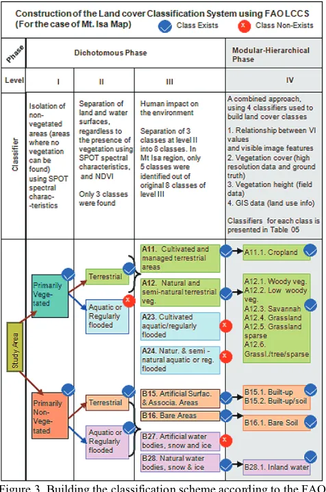
Figure 3. Building the classification scheme according to the FAO LCCS.

4.2.1 Classification Level I: A supervised classification to isolate non-vegetated lands was conducted through careful selection of training sites from 100% non-vegetated areas. Spectral values of each SPOT band and NDVI image together with 2.5m SPOT images were used to identify these training sites, precisely. All other areas under different levels of vegetation (from vegetated area to a mix of bare ground and grass) were classified into vegetated areas.

4.2.2 Classification Level II: The re-classification was carried out with two classes of level I to generate four classes. After observing the NDVI, image classification was conducted through selecting training sites using the 2.5m and 10m SPOT images. Only 3 classes were found out of four, and the class A2 (“aquatic or regularly flooded areas under primarily vegetated category”) (see figure 3) were not found in Mt Isa region.

4.2.3 Classification Level III: At this level, FAO LCCS has 8 sub classes to represent all land surface features on the earth. The availability of the area under each class is directly depending on the regional features of land cover of each respective area. A clear example is, in a remote desert region with no human settlements or any vegetation, it may just comprise of only one class (B16, A6: Loose and Shifting Sand) from these 8 classes. The Mt Isa region has a predominantly dry climate and no vegetated lands under aquatic or regularly flooded conditions exit. We found five classes out of eight original classes at this level (see Level III in figure 3) with regard to Mt Isa region.

4.2.4 Classification Level IV: The 4th level of the classification is the challenging phase of the land cover mapping, which must identify classes closer to real world land cover with clearly demarcated boundaries. As an example, even after extensive studies, the LCC for Tasmania conducted in 2006 had 14 classes at local level, but one of them, “seabird rookery complex” found no matching class in FAO LCCS to be re-named (Atyeo and Thackway 2006). Fundamentally, the 4th level or local level class generation has to be conducted through applying more detail “classifiers” (Di Gregorio, 2005), as FAO LCCS requires. In this study we used very high resolution 2.5m satellite images and ground survey information to build classifiers for the 4th level. Additionally, spectral characteristics of SPOT 10m images played a strong role in the classification process. Figure 3 shows the simplified flow of this process which presents all four levels with regard to the Mt. Isa map. Classifiers used to generate each class in level IV for Mt Isa map are presented in Table 05.

Table 05. Land cover classes mapped in Mt Isa region under FAO LCCS system

Class Code

Class name

Classifiers Corresponding FAO

LCCS classif. Code

A11.3 Crop

land

VIT(visually identified training sites using 2.5m images) + high NDVI value (around 0.6)

A11

A3 Herbaceous D4 Surface irrigated

A12.1 Woody

vege-tation

VIT + high NDVI value (higher than 0.3) + closed woodlands (> 60%) + tree height is over 2.5m

A12 A1 Woody A1 A10 Closed A10 B1 Height 7 – 2 m A12.2 Low

Woody vege-tation

VIT + high NDVI value (higher than 0.3) + open woodlands (10 – 40%+ tree height is over 1m

A12 A1 Woody A21 Open B14 Height 5 – 05m

A12.3 Savan-

nah

VIT + areas under low NDVI value (below or around 0.3), and Shrubs (Sparse) + Graminoids observed from field investigation

A12 A4 Shrub A6 Graminoids A14 Sparse (1% - 15% Shrubs and trees)

A12.4 Grass

land (wetlan ds)

VIT + areas with moderate to high NDVI value (0.3 - 05), dominate by Graminoids observed from field investigation

A12

A6 Graminoids C1Spatial distribution

A12.5 Grass

land sparse

Visually identified training sites from areas under low NDVI value (below 0.3), with Sparsely distributed Graminoids, observed from field investigation

A12

A6 Graminoids A14 Sparse

A12.6 Grass

land /tree/ sparse

Special spectral feature of soil color caused by rocky terrain, identified by 10m and 2.5m data, verified by field investigations.

A12, A6 Graminoids A4 Shrubs, A14 Sparse A3 Tree Sparse

B15.1

Built-up

Visually identified training sites using 2.5m data and field investigation

B15

Urban Areas A13

B15.2

Built-up/soil

B15

A12 Industrial and other

B16.1 Bare

soil

B16

A5 Unconsolidated Bare soil

B28.1 Inland

water

Visually identified training sites using 2.5m data

B28. A1 Water A1

5. RESULTS OF THE CASE STUDIES

This paper mainly emphasizes the characteristics of Australian land surface and the application of FAO LCCS to classify that into

land cover classes. We produced land cover maps for the two test sites mentioned in previous sections.

5.1 Mt. Isa, the arid region

The vicinity of Mt Isa city significantly represents the vast inner Australian arid landscape. The centre of the mapped area (Mt Isa city) associates with a large mining complex, which is one of the largest in Australia. The built-up area of the city with 23,000 people is restricted to a small area, though its urban limits cover 43,310 square kilometres (moutisa.qld.gov web). Due to the harsh climate, no major farming areas can be seen closer to the city, except ranching activities. Figure 4 A and B, shows typical red-soil outback (Australian term for remote area) environment around Mt Isa.

Figure 4. Typical land cover types in Mt Isa area. Left area is about 7 km east and right area is 18 km south to the Mt. Isa city.

Through a careful observation of spectral characteristics of SPOT 10m images and vegetation index images as explained in section 3.3, a land cover map of Mt Isa was produced with 11 classes under the 4th _{level (figure 5). An accuracy assessment of} the Mt Isa map was carried out using the 2.5m SPOT image. Using a systematic random sample, 128 points were selected from the area covered by 2.5m image and checked against the classified image data. Samples were under represented on land cover types with very low areas of coverage, but all major land cover types were counted. Results showed an overall accuracy of 82% for Mt Isa map.

5.2 Brisbane, the coastal urban region

Mapping urban environments using high resolution satellite data is a relatively an easy task, since spectral characteristics of urban surface show a clear discrimination against vegetation. Specially, Brisbane city stands out clearly against the surrounding mostly non-built-up areas of Queensland. The map shown here as Brisbane (figure 6), is a subsection of a larger map that covers whole southeast Queensland (SEQ) catchment. SEQ has a wide variety of land cover types and its Brisbane-Gold Coast coastal urban belt with over 1.5 million people (2007 Projected) (ABS, Australia) is the busiest urban region in the northern half of Australia. Table 06 presents land cover classes mapped in Brisbane area, under FAO LCCS.

An error matrix was used on the classified SEQ map to determine the percentage of land cover accuracy. The error matrix used a total of 190 points and found total class accuracy for the entire SEQ Catchments area was 90%. The selected subregion in this study may have a different accuracy, if a separate sample is administrated for the subregion only. Specifically, the accuracy of the separate built-up areas from vegetated lands is high, compared to finding boundaries amongst vegetation types. Also, the inclusion of GIS data layers into the final map of SEQ has forced the vegetation types into some mixed vegetation classes (e.g., Tree Plantations), which is not a typical land cover class able to be identified through spectral classifications only.

5.3 The qualitative aspects of new maps

This study was conducted to apply the FAC LCCS system for Australian land cover products. Initially, two full SPOT image scenes were classified and only sub-regions of 1000skm were

presented in this study in order to present clearer maps. To maintain homogeneity within each land cover class, classes have to be built with broad and easy to understand classifiers. A large number of classes based on micro-level local information is appropriate for local level detail mapping, and such a scheme must be organized in order to be accommodated within the national level land cover maps.

Figure 5. Land cover map of Mt Isa region.

Table 06. Land cover classes of Brisbane area under FAO LCCS. Class Code

(Arranged by FAO LCCS)

Class name

Brisbane (South East Queensland)

A11.1. Grassland - farm

A11.2. Tree Plantation

A11.3. Cropland - Dry land

A11.4. Cropland - Irrigated

A11.5. Cropland – Tree crop

A12.1. Medium to tall woody veg.

A12.2. Woody open

From A12.3. to A12.10

No class identified

B15.1 Built-up-Non-vegetated

B15.2 Built-up-Impervious road surface

B15.3 Non-built-up non vegetated

B15.4 Non-built-up-Mine/Quarry

B15.5 Non-built-up-Impervious road surface

B16.1 Bare rock (only in outside of selected area)

B16.2 Bare soil

B27.1 Canals

B28.1 Inland water

We have used an approach based on spectral values and visual observation of super-resolution (2.5m colour images), which are the basic needs for any classification. We then added field observation information to the training site selection and the refining process, which strengthens the classifiers used to break level 3 classes into the 4th or final level classes. As explained earlier, the classification gave satisfactory levels of accuracy with both maps being accommodated in a classification scheme based on FAO system. Figure 7 visually compares new map with existing SLATS 2001-2003 data set to indicate the improvement in land cover data when high resolution images were used.

Figure 6. Land cover map of Brisbane urban region.

Figure 7. Comparison of land cover details of a sample area.

6. CONCLUSIONS

Australia’s agriculture and mining based economy requires an accurate assessment of land use and land cover. However, mapping the country at 10m or finer resolution has just started and

over 90% of the country is yet to be mapped. This study classified two distinctly different landscape plots from Queensland, Australia. The prime objective of the study was to build the classification system common for both regions using the fundamental approach of FAO Land Cover classification system. The FAO system has three initial class levels based on a priori (pre-defined) classification approach and the 4th detail level or the Modular-Hierarchical Phase. A careful observation of the spectral information against super resolution satellite data and ground survey information enabled classifiers for 4th level to be selected. For each map, different land cover types were identified in diverse geo-physical and climatic conditions for each respective region. Some classes ended with same name and same class identifier when the classifiers were similar to each other (i.e.; A12.2. woody open class in Brisbane map). The results showed a promising outcome for mapping different regions under a single classification scheme. The maps were completed with a high accuracy and 10m spatial resolution which will be a useful data source for regional and national level land cover planning.

Acknowledgements:

Authors are thankful to Mr. Jeremy Hayden of Southern Gulf catchments for providing satellite data and facilitating field investigation opportunity in Mt. Isa region.

References:

1. Africover LCCS, FAO: 2008, online document,

http://www.broadsound.qld.gov.au/news/2007/LG_Reform_Cover page.shtml http://www.africover.org/LCCS_hierarchical.htms

2. Agro data; World Resource Institute, 2006

http://earthtrends.wri.org/text/agriculture-food/country-profile-9.html

3. Atyeo C. and Thackway R., 2006, Classifying Australian Land

Cover, Australian Government, Bureau of Rural Sciences

4. Australian Bureau of Statistics, 2008.

http://www.ausstats.abs.gov.au/ausstats/

5. Barrie Pittock, 2003, Climate Change: An Australian Guide to the

Science and Potential Impact. Australian Government agency on greenhouse matters, 94-101 pp

6. Climatemap www.bom.gov.au/climate/environ/other/kpn_all.shtml

7. Department of the Environment, Water, Heritage and the Art,

2008, Gondwana Rainforests of Australia,

8. http://www.environment.gov.au/heritage/places/world/gondwana/i

nformation.html

9. Di Gregorio A., FAO Land Cover Classification System,

Classification concepts and user manual, software version 02. 2005

10. Di Gregorio A.., and Jansen L. J. M., 2000: Lands cover

classification system (LCCS), FAO.

11. Hughes L., 2003, Climate change and Australia: trends, projections

and impacts. Austral Ecology 28, 423-443.

12. Hughes, L., 2005: Impacts of climate change on species and

ecosystems: an Australian perspective, The International Biogeography Soc., Summer 2005 Newslet.: Vol. 3, No. 2

13. Michael F.H., Sue M., Richard J. Hobbs, Janet L. Stein, Stephen G.

and Janine K.: 2005, Integrating a global agro-climatic classification with bioregional boundaries in Australia. Global Ecology and Biogeography, 14, 197-212

14. Mt Isa information,

http://www.mountisa.qld.gov.au/theIsa/lifestyle.shtml

15. National Land & Water Resources Audit, Australian land cover

mapping, 2007

16. Peter Butt, 2001: Land Law, Law Book Co of Australasia, 2001

http://www.teamlaw.org/LandDef.htm

17. Population datahttp://www.ausstats.abs.gov.au/

18. Soil map information

http://www.cazr.csiro.au/connect/resources.htm

19. State of the Environment, 2001: Independent Report to the

Commonwealth Minister for the Environment and Heritage. Australian State of the Environment Committee. Land and Vegetation section, www.environment.gov.au/soe/2006

20. Weather data,

www.bom.gov.au/climate/averages/tables/cw_040214.shtml