Toolpath interpolation and smoothing for computer numerical control machining of freeform surfaces : a review

Toolpath Interpolation and Smoothing for Computer

Numerical Control Machining of

Freeform Surfaces: A Review

Wen-Bin

Zhong

Xi-Chun

Luo

Wen-Long

Chang

Yu-Kui

Cai

Fei

Ding

Hai-Tao

Liu

Ya-Zhou

Sun

1 Centre for Precision Manufacturing, Department of Design, Manufacture & Engineering Management (DMEM), University of Strathclyde, Glasgow G1 1XJ, UK

2 Engineering and Physical Sciences Research Council (EPSRC) Future Metrology Hub, Centre for Precision Technologies, University of Huddersfield, Huddersfield HD1 3DH, UK

3 School of Mechatronic Engineering, Harbin Institute of Technology, Harbin 150001, China

Abstract:   Driven by the ever increasing demand in function integration, more and more next generation high value-added products, such as head-up displays, solar concentrators and intra-ocular-lens, etc., are designed to possess freeform (i.e., non-rotational symmetric) surfaces. The toolpath, composed of high density of short linear and circular segments, is generally used in computer numerical control (CNC) systems to machine those products. However, the discontinuity between toolpath segments leads to high-frequency fluctuation of feedrate and acceleration, which will decrease the machining efficiency and product surface finish. Driven by the ever-increasing need for high-speed high-precision machining of those products, many novel toolpath interpolation and smoothing approaches have been  pro-posed in both academia and industry, aiming to alleviate the issues caused by the conventional toolpath representation and  interpola-tion methods. This paper provides a comprehensive review of the state-of-the-art toolpath interpolation and smoothing approaches with systematic classifications. The advantages and disadvantages of these approaches are discussed. Possible future research directions are also offered.

Keywords:   Computer numerical control (CNC) , toolpath, interpolation, smoothing, freeform surface.

1

Introduction

Freeform surfaces are often defined as surfaces that

are non-rotationally symmetric[1]. 3D products with

free-form surfaces, such as impellers, optics, biomedical im-plants etc., have been widely used in areas like power,

semiconductor and medical[2–4]. They are playing

increas-ingly important roles in improving our daily standards of living. For instance, thousands of hip, knee, ankle, elbow and shoulder joint replacement operations take place in

the UK every year[5], which bring pain relief and

mobil-ity improvement to many patients. Freefrom surfaces are often designed to satisfy or improve a specific functional requirement. Sub-micrometer form accuracy and nano-meter surface finish are often required to guarantee the designed functionality. Multi-axis computer numerical control (CNC) machining has been a key technology for

fabricating such surfaces. Fig. 1 illustrates how the

geo-metric data of freeform surfaces is converted to a CNC machining program in current practice. The product sur-face is firstly designed in computer-aided design (CAD) software. Then the computer-aided manufacturing (CAM) software is executed to convert the cutter con-tact (CC) path into the cutter location (CL) path. The CL path is usually divided into a large number of piece-wise linear and circular segments as the toolpath to guide the movement of machine axes. Given a sufficient num-ber of segments, the toolpath can approximate the origin-al surface accurately. Finorigin-ally, the CNC is responsible for interpolating the toolpath to finish the machining. This conventional toolpath representation method will result in the following undesirable problems:

1) The original freeform surface and CC path are rep-resented in continuous parametric form in CAD and CAM, as regulated by standards such as the initial

graphics exchange specification (IGES)[6] developed by

the American national standard, and the ISO 10303

standard[7] which is informally known as standard for the

exchange of product model data (STEP). However, only the linear interpolation (G01) and circular interpolation (G02 and G03), which are defined in the RS274D

stand-  Review

Special Issue on Improving Productivity Through Automation and Computing

Manuscript received March 20, 2019; accepted June 12, 2019 Recommended by Associate Editor Xian-Dong Ma

© The Author(s) 2019

International Journal of Automation and Computing

ard[8] and the ISO 6983 standard[9–11], are supported

across all CNCs. The discretization of continuous curves into linear and circular segments will inevitably

intro-duce the chord error, as shown in Fig. 2. There is a

trade-off between the toolpath approximation accuracy and the size of the part program. Shorter segments can decrease the chord error, but the number of segments will grow dramatically, which will pose a huge burden to the data transfer and CNC memory.

2) Due to the discontinuity of the linear and circular segments at the join points, the machine axes will experi-ence step velocity change at the corner. It requires infin-ite acceleration to achieve the movement, which will sat-urate the motor drives. Therefore, the conventional

lin-ear and circular interpolators have adopted the "S-curve"

velocity profiles, i.e., decrease the feedrate gradually when approaching the corner and start accelerating again at the beginning of the next segment. However, the fluc-tuation of feedrate and acceleration will decrease the av-erage feedrate and cause vibration, i.e., lower productiv-ity and surface finish. This problem will get even worse as high-density short segments are usually used when ma-chining freeform surfaces. Lengthy mama-chining time is of-ten expected, as an example, it took 42 hours to machine

a micro inducer as illustrated in Fig. 3. Moreover, the

un-desirable "dwell marks" will be left on the workpiece[14],

while good surface finish is often required.

The gap between the well-established freeform sur-faces representation method in CAD and the very lim-ited toolpath representation method in CNC has

attrac-ted a lot of attention since the 1990s. Fig. 4 illustrates a

promising solution to bridge the gap, where parametric curves are used as the toolpath for CNC. Mathematically, the parametric curve uses an explicit function of an inde-pendent parameter to define each coordinate

C(u) = (x(u), y(u), z(u)), a≤u≤b (1)

C(u)

where is the vector function of a curve with the

independent variable u, which is defined in the interval

[a, b].

Parametric representation exhibits many advantages

in CAD/CAM, as summarized by Piegl and Tiller[16],

most important advantages are that it is easy to extend to higher dimensions, intuitive for geometric design, etc. Therefore, it becomes the de facto standard for geomet-ric data exchange. It is also very convenient for multi-axis CNC control, where the reference point can be directly

calculated with the given parameter u. Compared with

CAM CNC

G/M codes

CAD Curve

segmentation Part program Motion planning

Reference points Control loops

Machine tool Linear/Circular real-time interpolator Line/Arc

segments

Curve representation

CAD model Cutter offset & path scheduling CL path

CC path

Fig. 1     Freeform surfaces data: from design to manufacturing (Adapted from [12])

Cutting tool _{Chord error}

CC path

Linear segment

Fig. 2     Chord error in conventional toolpath representation method

1 mm

500 mm 500 mm

Fig. 3     Micro inducer machined by 5-axis micro-milling[13]

Segmentation

Parametric curve represented

model

Parametric curve information

Parametric curve interpolator

Tool motion

Man-machine interface

device

CAD CNC

Fig. 4     Freeform  surface  machining  with  parametric interpolation[15]

the conventional linear and circular toolpath, it can avoid the cumbersome part program because it conveys much more information. And the high frequency fluctuation of the feedrate and acceleration can be eliminated due to the higher continuity provided by the parametric curve. Many different types of parametric curves are used for toolpath representation, such as pythagorean-hodograph

(PH) curves[17], NURBS (non-uniform rational

B-spline)[18], subdivision curves[19], etc. However, the

imple-mentation of these parametric curves remains a challenge. Proprietary parametric curve interpolation solutions are provided by some CNC manufacturers, but, they are not compatible with each other. The standard for parametric interpolation has not been finalized yet. Alternatively, the CNC built-in toolpath smoothing function can overcome the drawbacks of conventional toolpaths to some extent, while keeping the current toolpath generation approach unchanged, which can help avoid the high expense of spe-cialized CAM postprocessors and trainings for the new parametric interpolation on the factory floor.

This paper aims to provide a comprehensive review on the development of the toolpath interpolation and smoothing approaches. The technique routes are classi-fied, the advantages and disadvantages are discussed. The rest of the paper is organized as follows: The novel toolpath interpolation and smoothing approaches are re-viewed in Sections 2 and 3, respectively. Section 4 con-cludes the paper with discussions.

2

Parametric

toolpath

interpolation

2.1

Overview

Table 1 summarizes the interpolation features of five commercial CNC systems, which have been widely de-ployed in the industry. All the listed CNC systems sup-port two or more advanced interpolation methods for spe-cific parametric curves, in addition to the standard linear and circular interpolations. However, those methods are patented and use different kind of syntaxes, the imple-mentation details are not disclosed. Particularly, the posi-tion-velocity-time (PVT) interpolator has been promoted by Delta Tau and Aerotech, which is actually a cubic Hermite spline interpolation method, and it has seen its wide application in slow tool servo (STS) turning of

free-form surfaces[20–22].

The problem of parametric curve interpolation can be expressed as, given:

C(u)

1) the parametric curve ;

2) the command feedrate F;

3) the interpolation period T;

4) the current (k-th interpolation period) motion

status: feedrate fk and acceleration ak;

C(uk)

5) the current reference point .

C(uk+1)

Calculate the reference point for the next

in-terpolation period. And the result should be subject to

machine dynamics constraints and chord error

tolerance[23]:

1) Axial velocities and accelerations should be limited to avoid saturating the drive;

2) The jerk should be limited to avoid the excitation of vibrations in components in the machine assembly;

3) The chord error increases with feedrate and curvature, the feedrate should be limited to achieve high interpolation accuracy, while the productivity should be kept as high as possible.

Therefore, the parametric curve interpolation prob-lem becomes an optimization probprob-lem. The performance index is the total travel time along the curve, and the constraints include the machine dynamics and the chord error tolerance. There are two fundamental parts to be solved for the problem:

1) Parameter sampling, i.e., given the desired feedrate

fk+1, determine the value of the parameter uk+1, which

corresponds to the next reference point.

2) Feedrate scheduling, i.e., given the current motion status and constraints, determine the value of the

de-sired feedrate fk+1, which is used to calculate the next

reference point.

2.2

Parameter

sampling

Currently, there are two technical routes to establish the relationship between the feedrate and the parameter,

i.e., arc length parametrization and recursive Taylor′s

ex-pansion.

2.2.1 Arclengthparameterization

The feedrate is the differential of arc length over time, if the curve can be parameterized with respect to its arc length, then the parameter sampling will become straight-forward. However, the arc length parametrization is ex-tremely difficult, as it requires solving the inverse func-tion of the non-linear integral funcfunc-tion for arc length

evaluation[23]

s(u) =

∫ u a

_C˙_(u)du=

∫u a

√

˙

x(u)2+ ˙y(u)2+ ˙z(u)2du (2)

∥∥

where s is the arc length, a is the start value of the

parameter and computes the Euclidean Norm. Wang

Table 1    Interpolation feature of commercial CNCs

CNCs FANUC Series 30i[24] SIEMENS SINUMERIK

840D[25]

HEIDENHAIN iTNC

530[26]

Delta Tau Power

PMAC[27] Aerotech A3200[28]

Interpolation Line, Circle, Exponential, Helix, Involute, Cylindrical, NURBS

Line, Circle, Helix, Spline, Polynomial, Involute

Line, Circle, Helix, Spline

Line, Circle, PVT, Spline

Line, Circle, PVT, Bézier

and Yang[29] worked out a solution for near arc length

parameterization of a set of discrete points with a composite quintic spline, second order continuity was

achieved between each segment. Later, Wang et al.[30]

improved the idea by imposing additional constraint at the knots, third order continuity and no unwanted

oscillations were reported. Fleisig and Spence[31] extended

the work to five-axis machining, a near arc-length parameterized quintic spline was introduced to represent the tool position, while a near arc-length parameterized

quintic spherical Bézier was introduced to represent the

tool orientation, and the coordinated motion was accomplished with a reparameterization spline. However, for the given parametric curves, the near arc length parameterization will introduce geometric deviation to the original toolpath. Therefore, this technique is best suited for the postprocessor of CAM.

Farouki and Shah[32] introduced PH curves as the

toolpath for freeform surface machining. The PH curves are special parametric curves with the distinguishing property that their derivatives or hodographs satisfy the Pythagorean condition

˙

x(u)2+ ˙y(u)2+ ˙z(u)2=σ(u)2 (3)

σ(u)

where is a polynomial. This feature enables PH

curves to calculate their arc length analytically, which makes the parameter sampling much easier. Later,

Farouki et al.[33] extended the PH curve to three

dimensional machining.

Erkorkmaz and Altintas[34] proposed to use a feed

cor-rection polynomial to map the desired arc length to the correct curve parameter. The feed correction polynomial was obtained by applying a least square fit over the arc length and curve parameter values. A 7th order polyno-mial was generated for the correction purpose, and the second order continuity was achieved at the connection

boundaries, as shown in Fig. 5. This technique was later

incorporated in the development of more advanced

al-gorithms[35–37]. Similarly, Lei et al.[38] used a cubic or fifth

degree Hermit spline to map the arc length with the para-meter in each subinterval of the curve. This kind of tech-nique is carried out off-line and can be incorporated into the postprocessor of CAM.

2.2.2 RecursiveTaylor′sexpansion

To determine the sampled point for each

interpola-u(t)

V(t)

tion interval, the reparameterization of u with time t is

required. However, the solution of the required function is generally difficult to get, but its differential can be

derived with the following steps. The feedrate along

the curve is defined by[39]

V (t) = ds

dt =

(

ds du

) (

du dt

)

. (4)

Transforming the above equation yields

du dt =

V (t)

ds du

(5)

where the arc length differential equation is given by

ds du =

√

˙

x(u)2+ ˙y(u)2+ ˙z(u)2. (6)

Substituting (6) into (5) yields

du dt =

V (t)

√

˙

x(u)2+ ˙y(u)2+ ˙z(u)2

. (7)

Shpitalni et al.[40] proposed to apply Taylor′s

expan-sion around t = kT, i.e., the k-th interpolation period, to

(7), which yields the relationship between the feedrate and the parameter

uk+1=uk+Tu˙k+

(

T2

2

)

¨

uk+higher order terms (8)

˙

u du

dt u¨

d2 u dt2

where denotes and denotes . They have

deduced the first order approximation of the Taylor′s

expansion

uk+1=uk+

V(t)T

√

˙

x(uk)2+ ˙y(uk)2+ ˙z(uk)2

. (9)

They also pointed out that if the interpolation period

T is very small and the curve does not have small radii of

curvature, the first order approximation is adequate.

Fa-nuc has applied this work to its NURBS interpolator[41].

Cheng et al.[12] worked out the second order

approxima-tion for improved accuracy and applied it to their NURBS command generator

uk+1=uk+

V(t)T+

(

T2

2

) (

dV (t) dt

)

√

˙

x(uk)2+ ˙y(uk)2+ ˙z(uk)2

−

(V (t)T)2( ˙x(uk) ¨x(uk)+˙y(uk) ¨y(uk)+˙z(uk) ¨z(uk)) 2(x˙(uk)2+ ˙y(uk)2+ ˙z(uk)2)2

. (10)

Farouki and Tsai[42] compared the accuracy of the

Spline parameter u

Sk

s lk

o _{Arc displacement}

Actual displacement Feed correction polynomial

Fig. 5     Feed correction polynomial[34]

Taylor′s expansion method with the PH curve arc length parametrization method. A quintic PH curve with strong curvature variation and uneven parameterization was

used in the experiment. A constant feedrate of 1 000 ipm

(25 400 mm/min) and a sampling frequency of 512 Hz

(in-terpolation period ≈ 1.95 ms) were used for the

interpola-tion. The "step size" was defined as the distance

trav-elled along the curve within each interpolation period,

which should be a constant value of 0.032 552 in

(0.826 820 8 mm). The "arc length error" was defined as

the difference between the actual distance travelled along the curve and the ideal distance over a period of time.

Fig. 6 shows the results from the first and second order

Taylor′s expansion methods with the PH curve method.

The PH curve method can accurately realize the fixed step size and almost zero arc length error, as the arc length of the PH curve can be calculated analytically.

The Taylor′s expansion methods, however, exhibit

fluctu-ations in step size as well as arc length error. The second

order Taylor′s expansion method is a great improvement

over the first order method, the step size error and arc length error were decreased by roughly two orders of magnitude. Despite the advantages of the PH curve method, the lack of support in CAD/CAM limits its

ap-plications in the industry. On the contrary, the Taylor′s

expansion method can be applied to any parametric curves, but the fluctuation of feedrate is inevitable due to the truncation of the high order terms.

Yeh and Hsu[43] introduced a compensatory value for

the Taylor′s expansion method. The value was obtained

according to the distance between the previous interpola-tion point and an estimated point. The interpolainterpola-tion sim-ulation on a NURBS curve showed that the algorithm can reduce the feedrate deviation by 50 times compared

with the second order Taylor′s expansion method. Zhao

et al.[44] proposed the arc length compensated Taylor′s

ex-pansion (ACTE) method to eliminate the feedrate fluctu-ation caused by the truncfluctu-ation error. A 33% reduction in feedrate fluctuation was achieved compared with

conven-tional Taylor′s expansion. Chen et al.[45] developed the

augmented Taylor′s expansion (ATE) method for

B-spline curves. The Heun′s method[46], which is an

im-proved method for calculating the numerical solution to the initial value problem, was used to attain a better ap-proximation to the true parameter value, and was calib-rated using offline computed knot-length pairs. A more

accurate result than the second order Taylor′s expansion

was reported. Those compensation measures can improve the interpolation accuracy, but there is always a notice-able increase in computation time.

2.3

Feedrate

scheduling

The feedrate scheduling plays a vital role in obtaining satisfactory productivity by exploiting the dynamic cap-abilities of the machine tool along the parametric curve. It is a non-trivial optimization problem, which has been

extensively studied in robotic manipulator control[47–49].

The solution to the time-optimal problem usually

in-volves "bang-bang" control, i.e., at least one constraint

First order 1 000 ipm 32.9

32.7

32.5

32.3

Step size (10

−3 in)

Second order 1 000 ipm 32.560

32.556

32.552

32.548

0

−10

−20

−30

−40

Arc length error (10

−3 in)

0.05

0

−0.05

−0.15 −0.10

0 0.2 0.4 0.6 0.8 1.0 1.2 1.4 Time (s)

0 0.2 0.4 0.6 0.8 1.0 1.2 1.4 Time (s)

Fig. 6     Performance of the first and second order Taylor expansion method compared with the PH curve interpolator. The dashed lines are exact “reference” data from the PH curve method, while the solid lines are data from the Taylor′s expansion methods[42].

reaches its upper or lower bound throughout the motion.

Timar et al.[50] demonstrated that the square of the

time-optimal feedrate for a polynomial curve can be determ-ined as a piecewise-rational function of the curve para-meter, however, it is only subject to the prescribed

accel-eration bounds of each axis. Later, Timar and Farouki[51]

improved the idea by imposing the speed-dependent axis acceleration bounds arising from the output-torque char-acteristics of axis drive motors. This algorithm was imple-mented on an open-architecture software controller for 3-axis CNC milling.

Dong and Stori[52, 53] proposed a generalized two-pass

feedrate optimization algorithm. The global optimality was demonstrated by proving the local optimality of each

trajectory segment. Dong et al.[54] later extended the

bid-irectional scan algorithm by introducing the jerk con-straint for the feedrate optimization process. The im-proved algorithm can reduce overshoot errors by more than an order of magnitude over the conventional

ap-proach with constant feedrate and G-codes. Compared

with the time-optimal approach without jerk constraint, this algorithm can improve cornering errors by approxim-ately 50%. The effectiveness of this algorithm was attrib-uted to the suppression of high-frequency structural

excit-ations caused by the jerk, as illustrated in Fig. 7. The

di-mension of the optimization problem will be increased with the addition of the other constraints, and the time-optimal solution will no longer be achievable with those techniques. Therefore, near time-optimal solutions are favored with less computational burden.

0.6 0.4 0.2 0

−0.2 −0.4 −0.6

Magnitude (V)

0 1 2 3 4 5 6

Time (s)

1.6 1.4 1.2 1.0 0.8 0.6 0.4 0.2

Power density (V

2/Hz)

0

100

0 50 150 200 250 300 350 400 450 500 Frequency (Hz)

0.6 0.4 0.2 0

−0.2 −0.4 −0.6

Magnitude (V)

0 0.5 1.0 1.5 2.0 2.5 3.0 3.5 4.0 4.5 5.0 Time (s)

1.6 1.4 1.2 1.0 0.8 0.6 0.4 0.2

Power density (V

2/Hz)

0

100

0 50 150 200 250 300 350 400 450 500 Frequency (Hz)

0.6 0.4 0.2 0

−0.2 −0.4 −0.6

Magnitude (V)

0 1 2 3 4 5 6 7 8 9 Time (s)

1.6 1.4 1.2 1.0 0.8 0.6 0.4 0.2

Power density (V

2/Hz)

0

100

0 50 150 200 250 300 350 400 450 500 Frequency (Hz)

Fig. 7     Magnitude and power spectrum of acoustic signals among the trajectories with jerk constraint (top row), without jerk constraint (middle row) and G-code trajectory (bottom row). Left column: acoustic magnitude. Right column: power spectrum[54].

Yeh and Hsu[15] worked out the analytical

relation-ship between feedrate, radius of curvature and chord er-ror, and proposed to change feedrate adaptively to limit

the chord error. Yong and Narayanaswami[55] improved

the idea by detecting feedrate sensitive corners offline so that the chord error and acceleration constraints can be

satisfied simultaneously. Erkorkmaz et al.[37] introduced

the process mechanics constraint during the feedrate scheduling for freeform milling. A specific resultant cut-ting force was maintained by compucut-ting the workpiece-tool engagement along the workpiece-toolpath and setting local feedrate limits. The overall feedrate optimization scheme

is illustrated in Fig. 8. The toolpath is planned in

com-mercial CAM software, the cutting force can be pre-dicted from the tool engagement geometry and the local feedrate limit is imposed to confine the resultant cutting

force according to the cutting force model. Guo et al.[56]

added the axis tracking error to the constraints. They es-tablished the relationship between the tracking error and the input signal of the high-order servo system. They also proved that the tracking error constraint can be reduced to a constraint on a linear combination of the

accelera-tion and jerk. Jia et al.[57] tackled the servo-lag induced

contour error during feedrate scheduling for high-preci-sion machining.

The lookahead technique is an effective approach to solving the problem of feedrate scheduling with many

constraints[58]. Annoni et al.[59] split the NURBS curve

in-to several segments according in-to its curvature and a dif-ferent feedrate limit was chosen for each segment to ful-fill the constraints. Then, the lookahead module was used to calculate the final feedrate of a segment considering the segment length and the following segments. Beudaert

et al.[60] proposed the velocity profile optimization

(VPOp) method, the lookahead technique was used to calculate the necessary feedrate reduction to approach a

sharp corner. Jin et al.[61, 62] implemented the lookahead

method by calculating the length of deceleration re-peatedly at each interpolation period, which allows rapid

reaction to sensitive areas on the curve. Wang et al.[63]

developed a trigonometric velocity scheduling algorithm, which consisted of two lookahead processes. In the pre-in-terpolation lookahead phase, the curve was scanned and classified into three cases according to the feedrate vari-ation. The explicit feedrate scheduling functions were cal-culated in the following lookahead stage. Smaller chord error was achieved than the S-curve and cubic

polynomi-al feedrate scheduling methods. Zhong et polynomi-al.[23] developed

the real-time interpolator for parametric curves (RTIPC) with feedrate lookahead and acceleration lookahead, as

shown in Fig. 9. The feedrate lookahead module checks

feedrate limits along the curve considering the chord er-ror and maximum axis velocity constraints, then the ac-celeration module validates the initial lookahead results against jerk and maximum axis acceleration constraints. The lookahead length was dynamically adjusted to mimize the computation load. Ten times productivity in-crease was achieved compared with the linear interpolat-or, and smoother motion profiles than the PVT interpol-ator were reported as well.

2.4

PVT

interpolator

Instead of specifying the exact toolpath for the free-form surface machining, the PVT interpolator only re-quires the user to provide the start and end positions of each segment, the velocities at both ends, as well as the travelling time. The interpolator will use a third order polynomial to interpolate between the given positions and velocities

C(t) =a0+a1t+a2t2+a3t3, 0≤t≤T s (11)

C(t)

where is the curve with the time parameter t, Ts is

(a)

(e)

(b) (c) (d)

(f) (g)

(k) (j) (i)

(h)

Cutting process

Toolpath & drives

CAM model & CL data Tool engagement conditionEngagement Cutting force model Resultant

cutting force Force limit

Feed limit

Feedrate ṡ

ṡ

ṡ

s

s

s Cutting force overload!

Limit

Feed limits due to cutting

Feed limits due to drives y

x s lk+1

lk lk+2

CL point Sub-segments:

#1 #3 #2#4

Update

B-spline fitting & refinement u

û=f0s7+f1s6···+f7 Numerical evaluation point s Feed correction polynomial

rss rs

rsss r=r(u(s))

Geometric derivatives

Feasibility not guaranteed!

Limit

Limit

Feed profiling & final trajectory

G93 G01(160 Hz inverse time) X−43.75 Y−6.000 Z4.431 F9600 X−43.75 Y−5.999 Z3.384 F9600 …

G94

Optimized NC code

Position

command y

x

z

Time Trajectory interpolation

Optimized feed profile

Jerk limited feed profiling with uninterrupted accelerations

Fig. 8     Feedrate scheduling with process mechanics constraint[37]

{ai}

the total travelling time, are the coefficients of the

polynomial, and can be determined by the given boundary conditions

        

C(0) =a0

C(T s) =a0+a1T s+a2T s2+a3T s3 ˙

C(0) =a1 ˙

C(T s) =a1+ 2a2T s+ 3a3T s2

(12)

C(0) C(T s)

˙

C(0) C˙(T s)

where and are the start and end points and

and are the corresponding velocities. Unlike

the geometric toolpath, the PVT interpolator also incorporates the feedrate scheduling information

    

˙

C(t) =a1+ 2a2t+ 3a3t2 ¨

C(t) = 2a2+ 6a3t ...

C(t) = 6a3

(13)

˙

C(t) C¨(t) C...(t)

where , and are the velocity, acceleration

and jerk, respectively. The PVT interpolator can achieve very smooth motion profiles within each segment. However, it can only maintain velocity continuity at the boundaries, as the end velocity of current segment is the starting velocity of the next segment. The acceleration is not necessarily continuous at the boundaries, which will lead to vibration.

The PVT interpolator allows great flexibility for the user to control the geometric profiles and motion profiles,

but the machine dynamics and other constraints are not considered. The planned toolpath is not as intuitive as the parametric curves or the linear and circular toolpath, and the deviation between the planned toolpath and the CC path is difficult to calculate. Great care must be taken when using the PVT interpolator, or excessive geo-metric error or vibration will be resulted.

3

Toolpath

smoothing

techniques

3.1

Overview

Linear and circular segments are still widely used as the toolpath on the factory floor due to the straightfor-ward coding and good support from CNC. However, they are increasingly becoming the bottleneck of the high-speed high-precision machining of freeform surfaces. The CNC build-in toolpath smoothing algorithms have been extensively studied both in academia and industry, as they can help eliminate the fluctuation of feedrate and acceleration while keeping the current practice of CNC machining without further training on the operator and huge investment in the advanced CAM postprocessors.

The toolpath smoothing methods can be classified in-to local smoothing and global smoothing according in-to the smoothing scope. Local smoothing works with two adja-cent segments, while global smoothing can act on a group of segments. These methods can also be classified into curve-based smoothing and velocity blending smoothing according to the smoothing mechanism. Curve-based smoothing is a two-step solution. Firstly, a parametric curve is used either to connect two segments at the corner or to approximate a group of segments. Then, the specially designed parametric curve interpolator is used to interpolate the parametric curve. By contrast, the velo-city blending method is a one-step solution, which sched-ules the velocity profile of each axis directly at the corner and creates a smooth transition. Table 2 summarizes the recently developed toolpath smoothing methods.

The degree of continuity is usually used to evaluate the performance of smoothing algorithms. There are two kinds of continuity associated with a curve, i.e.,

geomet-ric continuity and parametgeomet-ric continuity[64]. If the n-th

derivatives of both curves at the join point have the same

direction, then Gn geometric continuity is achieved at the

join point. If the derivatives have the same magnitude as

well, then Cn parametric continuity is achieved. For

free-form surfaces machining applications, at least C2

continu-ity is required to guarantee continuous veloccontinu-ity and accel-eration along the toolpath.

3.2

Local

curve

corner

rounding

Table 2 shows that the majority of researchers fo-cused on the local curve corner rounding method, as it can solve the corner transition problem in an analytical

Given curve

C(u)

Calculate lookahead length

Feedrate lookahead

Acceleration

lookahead Intelligentactivation Buffer Multi-cases

No

No

Yes

Yes Calculate servo

reference point

Curve end

End

Special cases

Fig. 9     Overall  design  of  the  RTIPC  with  feedrate  and acceleration lookahead[23]

way, which minimizes the computational load for real-time CNCs. The SIEMENS SINUMERIK 840D sl

con-troller[65] implements its continuous path mode (G641

etc.) by inserting a spline at the corner. The Aerotech

A3200 controller[7] inserts a circular arc (ROUNDING

ON) for the corner transition, this measure can only

achieve G1 continuity, which means that the acceleration

is not continuous at the join points.

High order parametric curves are generally required to guarantee smooth motion profiles at the corner. The cu-bic spline was used by [60, 65, 70–72], while quintic

B-spline was adopted by [68, 72, 73]. Shi et al.[70] developed

their five-axis corner rounding method with a pair of

quintic PH curves. Bi et al.[71] realized the same purpose

with dual cubic Bézier curves. To discuss the advantages

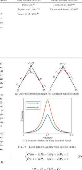
and disadvantages of the local curve corner rounding method, an example of corner rounding with a cubic B-spline is illustrated.

Fig. 10 (a) depicts a cubic B-spline curve is inserted

between the linear segments Q0Q1 and Q1Q2. Five

sym-metric control points are positioned on the linear

seg-ments. The knot vector {0, 0, 0, 0, 0.5, 1, 1, 1, 1} is

usu-ally used to create a symmetric B-spline curve. The max-imum deviation can be calculated analytically as

ε=∥P2−C(0.5)∥=

1

2P2− 1 4P1−

1 4P3

. (14)

The deviation can be easily controlled by carefully

po-sitioning P1 and P3. Since the first three and last three

control points are collinear, the new toolpath is G2 and

curvature continuous at the connecting points P0 and P4.

The smoothness can be further improved if the second de-rivatives of the B-spline at both ends are zero, as shown in (15). Equation (15) can be further simplified to (16),

which gives the positions of P0 and P4.

{

¨

C(0) = 12P2−36P1+ 24P0=0 ¨

C(1) = 12P2−36P3+ 24P4=0

(15)

{

P2−P1= 2 (P1−P0)

P2−P3= 2 (P3−P4).

(16)

It is obvious that this kind of approach is very re-strictive if the toolpath is composed of high density short linear segments, which are very common in the finish ma-chining of freeform surfaces. The inserted B-splines will overlap with each other, which makes the subsequent

in-terpolation impossible. Tulsyan and Altintas[72] proposed

P2=Q1 P2=Q1

P1 P₃

P3

P4

P4

P1

P0

P0

Q0 Q2 Q0 Q2

ε ε

(a) (b)

Curvature

0 0.5 1.0

Parameter

(a) Unrestricted transition length (b) Restricted transition length

(c) Curvature comparison of the transition curves

Fig. 10     Local corner rounding with cubic B-spline

Table 2    Summary of the recently developed toolpath smoothing methods

Local curve corner rounding Global curve approximation Local velocity blending Global velocity blending

SIEMENS[65] FANUC[77] Delta Tau[82] Tajima et al., 2018[85]

Aerotech[66] SIEMENS[65] Tajima et al., 2016[83] Tajima and Sencer, 2016[86]

Huang et al., 2017[67] Yang et al., 2015[78] Sencer et al., 2015[84] Yang and Yuen, 2017[68] Fan et al., 2015[79]

Sun et al., 2016[69] Wang et al., 2014[80]

Shi et al., 2015[70] Yuen et al., 2013[81] Bi et al., 2015[71]

Tulsyan and Altintas, 2015[72]

Sencer et al., 2014[73] Zhao et al., 2013[74] Beudaert et al., 2013[75]

Pateloup et al., 2010[76]

to restrict the length of the transition path to avoid the

overlap problem, i.e., the maximum length of P0P2 and

P2P4 are restricted to the minimum half-length of the

connecting segments, as shown in Fig. 10 (b). However,

this measure will lead to the over-constrained tolerance

and much higher curvature, as shown in Figs. 10 (b) and

10 (c). The feedrate must slow down to avoid saturating

drives at the corner.

3.3

Global

curve

approximation

The global curve approximation method can over-come the limitation of local curve corner rounding. However, it suffers from the difficulty of controlling the

approximation deviation. Piegl and Tiller[16] have carried

out some fundamental work on the B-spline approxima-tion. They proposed an iterative way to approximate a set of points and used the least squares technique to cal-culate the unknown control points. They pointed out that the approximation process was computationally intensive, and wiggles tended to exist in the final curve. Moreover, their method only considered controlling the deviation between the points and the curve, and the deviation within each segment is very likely to be enormous. To avoid this undesirable problem for high-precision free-form surface machining, the Hausdorff distance between the approximation curve and the original toolpath should

be used, as shown in Fig. 11. Hausdorff distance is used to

measure the distance between two subsets in mathemat-ics. In this scenario, the two subsets are the approxima-tion curve and the original toolpath, respectively.

The evaluation of Hausdorff distance is exceptionally

computationally intensive[87], which makes it very

re-strictive for real-time CNCs. The SIEMENS

SINU-MERIK 840D sl controller[65] implements its NC block

compression function (COMPCAD) by approximating consecutive linear segments with 5th degree NURBS. Users are warned that it is very processor and memory-intensive, and should be considered as the last resort

when other measures are not satisfactory. The FANUC

Series 30i-LB controller[77] implements its smooth

inter-polation function (G05.1) by fitting linear points using

cubic splines[89]. Fan et al.[79] developed the global

smoothing method using mixed linear and quartic Bézier

segments. Wang et al.[80] used the Akima curve to fit the

linear toolpath, only C1 continuity was achieved. Yuen et

al.[81] developed a five-axis linear toolpath smoothing

method using a quintic B-spline, the curve fitting

al-gorithm was based on the Piegl and Tiller′s method

without considering the Hausdorff distance.

3.4

Local

velocity

blending

Velocity blending based smoothing methods can achieve higher efficiency than curve-based smoothing methods as they eliminate the curve planning process. The one-step solution detects the corner and schedules axes velocities in the lookahead operation, as shown in

Fig. 12. However, it also has the same limitation as the

local curve corner rounding method. The Delta Tau

Power PMAC controller[82] achieves the fixed-error corner

blending by calculating the blending time based on the move speeds and change in angle at the corner. The blending starts and ends at the blending-time-dependent distance from the corner. The actual blending length will be very limited if the original linear segments are short, thus the feedrate must slow down to avoid saturating the

drives. Sencer et al.[84] developed a method using finite

impulse response (FIR) to filter the discontinuous axes velocities at the corner to achieve a smooth transition. The tolerance was controlled by selecting the

overlap-ping time. Tajima and Sencer[83] proposed the velocity

blending method based on the jerk limited acceleration profile (JLAP). The proposed algorithm was reported to be able to achieve better performance than the spline based corner rounding method by reducing the overall cycle time 6–7%.

3.5

Global

velocity

blending

Tajima and Sencer[86] later realized the limitation of

the local velocity blending method, and developed the look-ahead windowing (LAW) technique to overcome the overlapping problem at adjacent corners. Experiments showed that the improved algorithm can reduce the cycle time up to 45% more than the point to point linear

inter-polation and 10–15% compared to the local Bézier corner

rounding method and FIR based local velocity blending

method. Tajima et al.[85] applied the FIR filtering to a

multiple segmented toolpath, as shown in Fig. 13. The

contour error of filtering circular segments was also con-sidered. Experiments showed that it was able to reduce

the cycle time up to 20% compared with the local Bézier

corner rounding method[85].

Sup inf d (x, y)

xϵX, y ϵ Y

Sup inf d (x, y)

y ϵ Y, x ϵ X X

Y

Fig. 11     Hausdorff distance between curve X and curve Y [88]

4

Conclusions

This paper has provided a review of the toolpath in-terpolation and smoothing methods for CNC machining of freeform surfaces. The following conclusions can be

drawn:

1) The conventional toolpath comprised of linear and circular segments has become the bottleneck for high-speed high-precision machining of freeform surfaces, be-cause the high density short segments results in high

fre- 

Y

X Y

X

Vx

Vy

t

t

Vx

Vy

t

t

Fig. 12     Comparison of corner transition without and with velocity blending[82]

(a) Filtering of a rectangular velocity pulse

Velocity

Acceleration

v v′

a′ a′

j′

v′ s′

Time _{Tv Tv} Time

Tv Tv+T1

Tv+T1+T2 T1

T1 _T

1T1+T2 T1 T2

T2 _T 2 Rectangular vel. pulse

(L=FTv) (L=FTv)

* (Conv.)

* *

* (Conv.) T1

1

T1 F

T1 F T2

1

T2 1

T1T2 F T2

1

ddt

ddt ddt ddt

(b) Filtering of a trapezoidal velocity pulse Trap. vel. pulse

(c) Displacement profile generation by interpolation

∫′ _dτ

Displacement

Jerk

Trapezoidal vel. profile Trapezoidal acc. profile

L 0

Fig. 13     FIR filtering based velocity blending method[85]

quency fluctuation of feedrate and acceleration, which will decrease the productivity and product surface finish.

2) The parametric curve is the desirable toolpath rep-resentation method for freeform surface machining. It can preserve the surface information with high continuity and avoid the drawbacks of linear and circular segments. However, the parametric toolpath has not been included in the standard. Some CNC manufacturers support pro-prietary parametric toolpaths.

3) It is extremely difficult to achieve the time-optimal solution for the interpolation of parametric curves sub-ject to constraints of machine dynamics and accuracy. The arc length parametrization can achieve higher

inter-polation accuracy than the Taylor′s expansion method,

but the high computational cost makes it ideal for the offline postprocessor of CAM.

4) The lookahead technique has been an effective way for the feedrate scheduling for the parametric interpolat-or. The lookahead process allows the flexibility of adding various constraints to the interpolator.

5) PVT interpolation is actually a cubic Hermite spline interpolation, which allows users to specify the polynomial toolpath for freeform surface machining. However, the acceleration is not continuous at the bound-aries, and it is error-prone.

6) The CNC built-in toolpath smoothing algorithm can mitigate the problems of linear and circular segments, without changing current practice of CNC machining.

7) The local curve corner rounding method provides an analytical solution to the corner rounding problem, but it has severe limitation when smoothing high density short segments, which are very common in the finish ma-chining of freeform surfaces. The limitation is found in a) The adjacent corner transition path may overlap with each other and make the subsequent interpolation im-possible; b) Alternatively, the length of the transition path is constrained which leads to high curvature and the feedrate must slow down to avoid saturating drives.

8) The global curve approximation method can avoid the limitations of local curve corner rounding method. However, it suffers from the difficulty of controlling the Hausdorff distance between the original toolpath and the approximation curve.

9) The velocity blending method can achieve higher efficiency than the curve based smoothing methods, be-cause it schedules the velocity profile of each axis dir-ectly at the corner without planning a transition curve.

Based on the assessment of current literatures, some possible future work for the freeform surface machining are offered:

1) Little work can be found that deals with the pro-cess dynamics in the CNC interpolator for freeform sur-face machining, while more and more difficult-to-cut ma-terials are being used for the 3D product.

2) More work is needed to improve the interpolator so that it can suppress the chatter and severe tool wear with

embedded sensors.

3) Interpolators that can automatically correct free-form surface machining errors with on-machine metro-logy are highly desirable in some demanding applications.

4) The hybrid machining, which simultaneously ap-plies more than one machining processes on the work-piece, has been an emerging solution for high-efficiency and cost-effective machining of freeform surfaces. There is a gap in the CNC interpolation and toolpath representa-tion methods to accommodate more than one processes.

Acknowledgements

The authors acknowledge the support from the UK Engineering and Physical Sciences Research Council

(EPSRC) under the program (No. EP/K018345/1) and

the International Cooperation Program of China (No. 2015DFA70630).

Open

Access

This article is licensed under a Creative Commons At-tribution 4.0 International License, which permits use, sharing, adaptation, distribution and reproduction in any medium or format, as long as you give appropriate credit to the original author(s) and the source, provide a link to the Creative Commons licence, and indicate if changes were made.

The images or other third party material in this art-icle are included in the artart-icle’s Creative Commons li-cence, unless indicated otherwise in a credit line to the material. If material is not included in the article’s Creat-ive Commons licence and your intended use is not per-mitted by statutory regulation or exceeds the perper-mitted use, you will need to obtain permission directly from the copyright holder.

To view a copy of this licence, visit http://creative-commons. org/licenses/by/4.0/.

References

X. Jiang, P. Scott, D. Whitehouse. Freeform surface  char-acterisation – A fresh strategy. CIRPAnnals, vol. 56, no. 1, pp. 553–556, 2007. DOI: 10.1016/j.cirp.2007.05.132.

[1]

J. Chaves-Jacob, G. Poulachon, E. Duc. Optimal strategy for finishing impeller blades using 5-axis machining. The InternationalJournal of AdvancedManufacturing Tech-nology, vol. 58, no. 5–8, pp. 573–583, 2012. DOI: 10.1007/ s00170-011-3424-1.

[2]

F. Z. Fang, X. D. Zhang, A. Weckenmann, G. X. Zhang, C. Evans. Manufacturing and measurement of freeform optics. CIRP Annals, vol. 62, no. 2,  pp. 823–846,  2013. DOI: 10.1016/j.cirp.2013.05.003.

[3]

I. S. Jawahir, D. A. Puleo, J. Schoop. Cryogenic  machin-ing of biomedical implant materials for improved  function-al performance, life and sustainability. Procedia CIRP, vol. 46, pp. 7–14, 2016. DOI: 10.1016/j.procir.2016.04.133.

[4]

National Joint Registry. JointReplacementSurgery:The NationalJointRegistry, [Online], Available: https://www.

[5]

hqip.org.uk/, March 8, 2019.

U.S. Product Data Association. Initial Graphics Exchange Specification, IGES 5.3, 1996.

[6]

M. J. Pratt. Introduction to ISO 10303-the STEP  stand-ard for product data exchange. JournalofComputingand InformationScience inEngineering, vol. 1, no. 1, pp. 102–

103, 2001. DOI: 10.1115/1.1354995.

[7]

T. R. Kramer, F. M. Proctor, E. Messina. The NIST RS274NGC Interpreter –Version 3, Technical Report  NI-STIR 6556, Department of Commerce, USA, 2000.

[8]

Automation Systems and Integration - Numerical Control of Machines - Program Format and Definitions of Address Words - Part 1: Data Format for Positioning, Line Motion and  Contouring  Control  Systems,  ISO  6983-1:  2009, December 2009.

[9]

Y. Zhang, X. L. Bai, X. Xu, Y. X. Liu. STEP-NC based high-level  machining  simulations  integrated  with CAD/CAPP/CAM. InternationalJournalofAutomation and Computing,  vol. 9,  no. 5,  pp. 506–517, 2012.  DOI: 10.1007/s11633-012-0674-9.

[10]

B. Venu, V. R. Komma, D. Srivastava. STEP-based  fea-ture recognition system for B-spline surface features.  Inter-national Journalof AutomationandComputing, vol. 15, no. 4, pp. 500–512, 2018. DOI: 10.1007/s11633-018-1116-0.

[11]

M. Y. Cheng, M. C. Tsai, J. C. Kuo. Real-time NURBS command generators for CNC servo controllers.  Interna-tionalJournalofMachineToolsandManufacture, vol. 42, no. 7,  pp. 801–813,  2002.  DOI:  10.1016/S0890-6955(02) 00015-9.

[12]

K. Nakamoto, T. Ishida, N. Kitamura, Y. Takeuchi.  Fab-rication of microinducer by 5-axis control ultraprecision micromilling. CIRP Annals, vol. 60, no. 1, pp. 407–410, 2011. DOI: 10.1016/j.cirp.2011.03.021.

[13]

S. J. Yutkowitz. Apparatus and Method for Smooth  Cor-nering in A Motion Control System, U.S. Patent 6922606, July 2005.

[14]

S. S. Yeh, P. L. Hsu. Adaptive-feedrate interpolation for parametric curves with a confined chord error.  Computer-Aided Design,  vol. 34,  no. 3,  pp. 229–237,  2002.  DOI: 10.1016/S0010-4485(01)00082-3.

[15]

L. Piegl, W. Tiller, TheNURBSBook, 2nd ed., New York, USA: Springer-Verlag, 1996.

[16]

Y. F. Tsai, R. T. Farouki, B. Feldman. Performance  ana-lysis of CNC interpolators for time-dependent feedrates along PH curves. Computer Aided Geometric Design, vol. 18,  no. 3,  pp. 245–265,  2001.  DOI:  10.1016/S0167-8396(01)00029-2.

[17]

C. Brecher, S. Lange, M. Merz, F. Niehaus, C. Wenzel, M. Winterschladen, M. Weck. NURBS based ultra-precision free-form  machining.  CIRP Annals,  vol. 55,  no. 1, pp. 547–550, 2006. DOI: 10.1016/S0007-8506(07)60479-X.

[18]

A. Vijayaraghavan, A. Sodemann, A. Hoover, J. Rhett Mayor, D. Dornfeld. Trajectory generation in high-speed, high-precision micromilling using subdivision curves.  In-ternational Journal of Machine Tools andManufacture, vol. 50, no. 4, pp. 394–403, 2010. DOI: 10.1016/j.ijmachtools. 2009.10.010.

[19]

Z. Q. Yin, Y. F. Dai, S. Y. Li, C. L. Guan, G. P. Tie.  Fab-rication of off-axis aspheric surfaces using a slow tool servo. InternationalJournalofMachineToolsand Manu-facture, vol. 51, no. 5, pp. 404–410, 2011. DOI: 10.1016/ j.ijmachtools.2011.01.008.

[20]

X. S. Wang, X. Q. Fu, C. L. Li, M. Kang. Tool path  gener-ation for slow tool servo turning of complex optical  sur-faces. TheInternationalJournalofAdvanced Manufactur-ing Technology, vol. 79, no. 1–4, pp. 437–448, 2015. DOI: 10.1007/s00170-015-6846-3.

[21]

L. Lu, J. Han, C. Fan, L. Xia. A predictive feedrate  sched-ule method for sculpture surface machining and  corres-ponding B-spline-based irredundant PVT commands  gen-erating method. The International Journalof Advanced ManufacturingTechnology, vol. 98, no. 5–8, pp. 1763–1782, 2018. DOI: 10.1007/s00170-018-2180-x.

[22]

W. B. Zhong, X. C. Luo, W. L. Chang, F. Ding, Y. K. Cai. A real-time interpolator for parametric curves.  Interna-tional Journal of Machine Tools and Manufacture, vol. 125, pp. 133–145, 2018. DOI: 10.1016/j.ijmachtools. 2017.11.010.

[23]

FANUC Corporation. FANUC Series 30i/31i/32i/35i –

MODELB, [Online], Available: https://www.fanuc.co.jp/ en/product/cnc/fs_30i-b.html, March 8, 2019.

[24]

Siemens AG. SIEMENSSINUMERIK840DslBrochure, [Online],  Available:  https://www.industry.usa.siemens. c o m / d r i v e s / u s / e n / c n c / s y s t e m s - a n d - p r o d u c t s / Documents/Brochure-SINUMERIK-840D-sl.pdf,  March 8, 2019.

[25]

HEIDENHAIN  Corporation.  HEIDENHAN iTNC 530 Brochure, [Online], Available: https://www.heidenhain.de/ f i l e a d m i n / p d b / m e d i a / i m g / 8 9 5 8 2 2 - 2 5_i T N C 5 3 0_

Design7_en.pdf, March 8, 2019.

[26]

Delta Tau Data Systems Inc. PowerPMACUser′s Manu-al,  [Online],  Available:  https://www.deltatau.com/ manuals/, March 8, 2019.

[27]

Aerotech Inc. Automation3200Brochure, [Online],  Avail-able:  https://www.aerotech.co.uk/product-catalog/ motion-controller/a3200.aspx, March 8, 2019.

[28]

F. C. Wang, D. C. H. Yang. Nearly arc-length  parameter-ized quintic-spline interpolation for precision machining. Computer Aided Geometric Design,  vol. 25,  no. 5, pp. 281–288, 1993. DOI: 10.1016/0010-4485(93)90085-3.

[29]

F. C. Wang, P. K. Wright, B. A. Barsky, D. C. H. Yang. Approximately Arc-length parametrized C3 quintic  inter-polatory splines. Journalof Mechanical Design, vol. 121, no. 3, pp. 430–439, 1999. DOI: 10.1115/1.2829479.

[30]

R. V Fleisig, A. D. Spence. A constant feed and reduced angular acceleration interpolation algorithm for  multi-ax-is machining. JournalofMechanicalDesign, vol. 33, no. 1, pp. 1–15, 2001. DOI: 10.1016/S0010-4485(00)00049-X.

[31]

R. T. Farouki, S. Shah. Real-time CNC interpolators for Pythagorean-hodograph curves. ComputerAided Geomet-ricDesign, vol. 13, no. 7, pp. 583–600, 1996. DOI: 10.1016/ 0167-8396(95)00047-X.

[32]

R. T. Farouki, M. Al-Kandari, T. Sakkalis. Hermite  inter-polation by rotation-invariant spatial  pythagorean-hodo-graph curves. Advances inComputationalMathematics, vol. 17,  no. 4,  pp. 369–383,  2002.  DOI:  10.1023/A: 1016280811626.

[33]

K. Erkorkmaz, Y. Altintas. Quintic spline interpolation with minimal feed fluctuation. Journalof Manufacturing ScienceandEngineering, vol. 127, no. 2, pp. 339–349, 2005. DOI: 10.1115/1.1830493.

[34]

K. Erkorkmaz, M. Heng. A heuristic feedrate optimization strategy  for NURBS toolpaths. CIRP Annals,  vol. 57, no. 1, pp. 407–410, 2008. DOI: 10.1016/j.cirp.2008.03.039.

[35]

M. Heng, K. Erkorkmaz. Design of a NURBS interpolator with minimal feed fluctuation and continuous feed  modu-lation capability. InternationalJournalofMachineTools andManufacture, vol. 50, no. 3, pp. 281–293, 2010. DOI: 10. 1016/j.ijmachtools.2009.11.005.

[36]

K. Erkorkmaz,  S.  E.  Layegh,  I.  Lazoglu,  H.  Erdim. Feedrate optimization for  freeform milling considering constraints from the feed drive system and process  mech-anics. CIRPAnnals, vol. 62, no. 1, pp. 395–398, 2013. DOI: 10.1016/j.cirp.2013.03.084.

[37]

W. T. Lei, M. P. Sung, L. Y. Lin, J. J. Huang. Fast  real-time NURBS path interpolation for CNC machine tools. InternationalJournalofMachineToolsandManufacture, vol. 47,  no. 10,  pp. 1530–1541,  2007.  DOI:  10.1016/j. ijmachtools.2006.11.011.

[38]

Y. Koren, C. C. Lo, M. Shpitalni. CNC interpolators:  Al-gorithms and analysis. ManufacturingScienceand Engin-eering, vol. 64, pp. 83–92, 1993.

[39]

M. Shpitalni, Y. Koren, C. C. Lo. Realtime curve  interpol-ators. Computer-aidedDesign, vol. 26, no. 11, pp. 832–838, 1994. DOI: 10.1016/0010-4485(94)90097-3.

[40]

T. Otsuki, H. Kozai, Y. Wakinotani. Free-form Curve  In-terpolation Method and Apparatus, U.S. Patent 5815401, September 1998.

[41]

R. T. Farouki, Y. F. Tsai. Exact taylor series coefficients for variable-feedrate CNC curve interpolators.  Computer-Aided Design,  vol. 33,  no. 2,  pp. 155–165,  2001.  DOI: 10.1016/S0010-4485(00)00085-3.

[42]

S. S. Yeh, P. L. Hsu. The speed-controlled interpolator for machining parametric  curves.  Computer-aided Design, vol. 31,  no. 5,  pp. 349–357,  1999.  DOI:  10.1016/S0010-4485(99)00035-4.

[43]

H. Zhao, L. M. Zhu, H. Ding. A parametric interpolator with minimal feed fluctuation for CNC machine tools  us-ing arc-length compensation and feedback correction.  In-ternational Journal of Machine Tools andManufacture, vol. 75,  pp. 1–8, 2013.  DOI: 10.1016/j.ijmachtools.2013. 08.002.

[44]

M. Chen, W. S. Zhao, X. C. Xi. Augmented Taylor′s  ex-pansion method for B-spline curve interpolation for CNC machine tools. InternationalJournalofMachineToolsand Manufacture, vol. 94, pp. 109–119, 2015. DOI: 10.1016/j. ijmachtools.2015.04.013.

[45]

Wikipedia.  Heun′s  Method,  [Online],  Available: https://en.wikipedia.org/wiki/Heun%27s_method,  May 20, 2019.

[46]

J. E. Bobrow. Optimal robot plant planning using the  min-imum-time criterion. IEEEJournalonRoboticsand Auto-mation, vol. 4, no. 4, pp. 443–450, 1988. DOI: 10.1109/56. 811.

[47]

G. Pardo-Castellote, R. H. Jr. Cannon. Proximate  time-optimal algorithm for on-line path parameterization and modification. In ProceedingsofIEEEInternational Con-ferenceonRoboticsandAutomation, IEEE, Minneapolis, USA,  pp. 1539–1546,  1996.  DOI:  10.1109/ROBOT. 1996.506923.

[48]

D. Verscheure, B. Demeulenaere, J. Swevers, J. De  Schut-ter, M. Diehl. Time-optimal path tracking for robots: A convex  optimization  approach.  IEEE Transactions on Automatic Control, vol. 54, no. 10, pp. 2318–2327, 2009. DOI: 10.1109/TAC.2009.2028959.

[49]

S. D. Timar, R. T. Farouki, T. S. Smith, C. L. Boyadjieff.

[50]

Algorithms for time-optimal control of CNC machines along curved tool paths. Robotics and Computer-Integ-ratedManufacturing, vol. 21, no. 1, pp. 37–53, 2005. DOI: 10.1016/j.rcim.2004.05.004.

S. D. Timar, R. T. Farouki. Time-optimal traversal of curved paths by Cartesian CNC machines under both  con-stant and speed-dependent axis acceleration bounds.  Ro-botics and Computer-integrated Manufacturing, vol. 23, no. 5, pp. 563–579, 2007. DOI: 10.1016/j.rcim.2006.07.002.

[51]

J. Dong, J. A. Stori. Optimal feed-rate scheduling for  high-speed contouring. Journalof ManufacturingScience and Engineering,  vol. 129,  no. 1,  pp. 63–76, 2004.  DOI: 10. 1115/1.2280549.

[52]

J. Dong, J. A. Stori. A generalized time-optimal  bidirec-tional scan algorithm for constrained feed-rate  optimiza-tion. Journal of Dynamic Systems, Measurement, and Control,  vol. 128,  no. 2,  pp. 379–390,  2006.  DOI:  10. 1115/1.2194078.

[53]

J. Y. Dong, P. M. Ferreira, J. A. Stori. Feed-rate  optimiza-tion with jerk constraints for generating minimum-time trajectories. InternationalJournal of MachineToolsand Manufacture, vol. 47, no. 12–13, pp. 1941–1955, 2007. DOI: 10.1016/j.ijmachtools.2007.03.006.

[54]

T. Yong, R. Narayanaswami. A parametric interpolator with confined chord errors, acceleration and deceleration for NC machining. Computer-aidedDesign, vol. 35, no. 13, pp. 1249–1259, 2003. DOI:  10.1016/S0010-4485(03)00043-5.

[55]

J. X. Guo, K. Zhang, Q. Zhang, X. S. Gao. Efficient  time-optimal feedrate planning under dynamic constraints for a high-order CNC servo system. Computer-aided Design, vol. 45,  no. 12,  pp. 1538–1546,  2013.  DOI:  10.1016/j. cad.2013.07.002.

[56]

Z. Y. Jia, D. N. Song, J. W. Ma, G. Q. Hu, W. W. Su. A NURBS interpolator with constant speed at  feedrate-sens-itive regions under drive and contour-error constraints.  In-ternational Journal of Machine Tools andManufacture, vol. 116,  pp. 1–17,  2017.  DOI:  10.1016/j.ijmachtools. 2016.12.007.

[57]

S. H. Suh, S. K. Kang, D. H. Chung, I. Stroud. Theoryand Design of CNC Systems, London, UK: Springer, 2008. DOI: 10.1007/978-1-84800-336-1.

[58]

M. Annoni, A. Bardine, S. Campanelli, P. Foglia, C. A. Prete. A real-time configurable NURBS interpolator with bounded acceleration, jerk and chord error.  Computer-aided Design,  vol. 44,  no. 6,  pp. 509–521,  2012.  DOI: 10.1016/j.cad.2012.01.009.

[59]

X. Beudaert, S. Lavernhe, C. Tournier. Feedrate  interpol-ation with axis jerk constraints on 5-axis NURBS and G1 tool path. International Journal of Machine Tools and Manufacture, vol. 57,  pp. 73–82, 2012.  DOI: 10.1016/j. ijmachtools.2012.02.005.

[60]

Y. A. Jin, Y. He, J. Z. Fu. A look-ahead and adaptive speed control algorithm for parametric interpolation. The InternationalJournal of AdvancedManufacturing Tech-nology, vol. 69, no. 9-12, pp. 2613–2620, 2013. DOI: 10. 1007/s00170-013-5241-1.

[61]

Y. A. Jin, Y. He, J. Z. Fu, Z. W. Lin, W. F. Gan. A  fine-in-terpolation-based parametric interpolation method with a novel  real-time  look-ahead  algorithm.  Computer-aided Design, vol. 55, pp. 37–48, 2014. DOI: 10.1016/j.cad.2014. 05.002.

[62]

Y. S. Wang, D. D. Yang, R. L. Gai, S. H. Wang, S. J. Sun.

[63]