Optimal array filtering for seismic inversion

(1)

Optimal Array Filtering

for

Seismic Inversion

Phillip Musumeci

B.E. Hons. M.Eng.Sc. (JCUNQ)

April 1989

A thesis submitted for the degree of Doctor of Philosophy of the Australian National University

(2)

These doctoral studies were conducted under the supervision of Dr. D.

Williamson.

The content of this thesis, except as otherwise explicitly stated, is the

result of original research, and has not been submitted for a degree at any

other university or institution.

Much of the work in this thesis has been published as academic papers

(see [20, 21, 22, 23]).

Canberra, April 1989.

Phillip Musumeci,

Department of Systems Engineering,

Research School of Physical Sciences,

The Australian National University,

(3)

Science is at no moment quite right, but it is seldom quite wrong,

and has, as a rule, a better chance of being right than the

the-ories of the unscientific. It is, therefore, rational to accept it

hypothetically.

(4)

Acknowledgements

I wish to thank my main supervisor, Dr. Darrell Williamson, for having

kept my project exciting for its 3 year duration. I have been particularly

lucky in this regard as my supervisor would not have been at ANU unless

the conditions were right to encourage him to take up his current fixed term

appointment (and to therefore discard his previously tenured position and to

take a cut in salary).

I also wish to thank the members of the Department of Systems

Engi-neering at ANU for giving me the opportunity for an Electrical EngiEngi-neering

education available at probably only a handful of places (one other located

in Australia). Unlike some Engineering Departments in Australia, this one

takes as one of its main aims the postgraduate education of students in

min-imum time. I am glad to have been part of this (time) efficient system.

My signal processing knowledge has been extended by Bon Clarke and

Panos Agathoklis, and my limited geological knowledge has been helped

con-siderably (i.e. created) by Steve Edwards and Greg Turner. I also

acknowl-edge assistance from Kok-Lay Teo.

I am grateful to the Australian National University for having managed

to keep in Australia (for the duration of this degree) my academic advisors

and the other members of the Department. This has been quite an

achieve-ment considering the opening overseas salary of PhD Electrical Engineering

(5)

Engineering at ANU (this salary is based on standard Australian Tertiary

Institution levels).

My funding has been provided primarily by an Australian Government

Postgraduate Award, with a supplementary scholarship originating from

BHP Pty. Ltd. While there appear to be few sectors of the Australian

community even vaguely aware that Engineering is connected to wealth

cre-ation as contrasted to its shuffling, I think that BHP in this instance deserve

special recognition for having sponsored this researchwithoutproprietary

re-strictions on publication and I hope that they are able to use the results to

commercial advantage. Optimal Array Filtering software has already been

shipped to BHP Central Research Laboratories for evaluation and as part of

the technology transfer associated with this project.

Canberra is a good place in which to live and work. A few people

de-serve special recognition for making it even better: Monty, Troy, and Grace

from ANU sports union for keeping the body fit; and Michael Frater, Lisa

Hamilton, and Alan Freeth for keeping the mind active with respect to a

broad range of topics by engaging in interesting and humorous argument.

Bob Bitmead and Jan Bitmead have been good friends. Thank you also to

my family.

My education has been positively influenced by a few people that I wish

to now mention: Osmond, Ridd, Close, Bitmead, and Williamson. The most

(6)

I think.

This Thesis is dedicated to the two-part dream that Australia should

have: (a) a National University; and (b) an Engineering School at our

Na-tional University designed specifically to improve the standards of

Under-graduate Education and Research in Australian Engineering. Unfortunately,

in 1989, the word ‘dream’ is used advisedly.

(7)

Abstract

This thesis considers two aspects within the broad seismic signal

process-ing field.

Optimal array filtering is studied in the context of seismic signal

analy-sis where off-line processing allows identification of signal parameters. The

filtering problem is formulated in the discrete time domain rather than the

frequency domain. It is shown that complete nulling of coherent

interfer-ence in the absinterfer-ence of sensor noise is generally possible with an array of FIR

filters. The order of each filter is determined from signal arrival times and

not duration. The filter design may also be optimised for operation in the

presence of random noise.

After the coherent interference is removed or attenuated, the resulting

sig-nals are used to identify the acoustic impedance profile between the source

and sensor. This problem is formulated as an identification problem

con-cerned with a one-dimensional lossy wave equation.

An analytic solution to the lossy wave equation is used to develop a

discrete space/discrete time model of seismic signal propagation through a

nonhomogeneous medium. The use of a finite spatial domain allows boundary

conditions to be explicitly included in the input-state-output model. A

one-step ahead recursive algorithm is presented for identification of the acoustic

impedance given finite data records. Given input/output information at

(8)

the transient period thus allowing identification based on the complete data

(9)

List of Figures

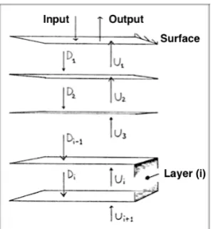
1.1 U and Dwaves in a layered media. . . 7

1.2 Seismic Data Acquisition. . . 14

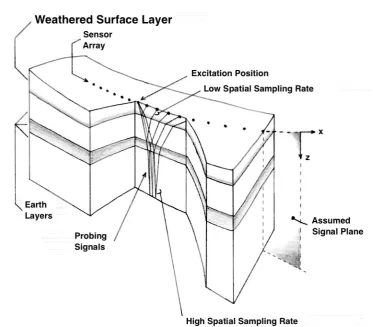
1.3 2D wave propagation. . . 25

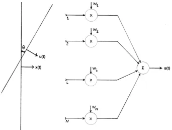
2.1 Narrowband Beamformer. . . 40

2.2 Array processing structure for absolutely optimal array filters. 44 2.3 Optimal Array Filters. . . 49

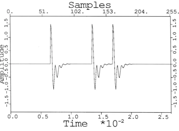
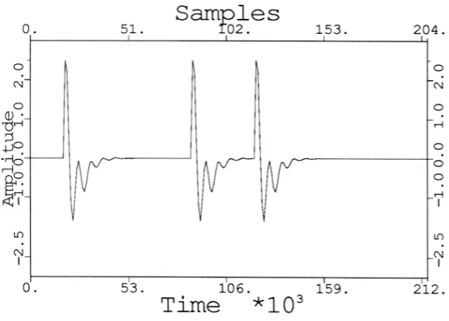
2.4 Wavelet x. . . 75

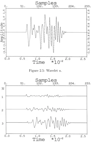
2.5 Wavelet u. . . 76

2.6 Test data for example 2.1. . . 76

2.7 Output (‘delay-and-sum’) for example 2.1(a). . . 77

2.8 Output (optimal) for example 2.1(b). . . 79

2.9 Output (suboptimal) for example 2.1(c). . . 79

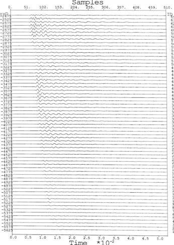
2.10 Seismic data set for example 2.2. . . 83

2.11 Windowed input data traces for example 2.2. . . 84

2.12 Output from optimal filter of example 2.2. . . 85

3.1 Test data set using u and w. . . 96

(12)

3.3 Array Filter (b) Output: designed using{x, u, w} data. . . 97

3.4 Output from 4 minimal optimal array filters. . . 109

3.5 Two-Dimensional Sensor Arrays. . . 112

3.6 Planar wavefront arrival producing rank(R) loss. . . 116

4.1 Seismic Mapping Problem. . . 129

4.2 System State with Recursion Integrals. . . 139

4.3 Discrete (ξ, t) and (µ, σ) meshes. . . 146

4.4 Response y0 given r(·) containing narrow spikes. . . 151

4.5 Response y0 and reflectivity r(·). . . 152

4.6 Response y0 given r(·) containing broad spikes. . . 153

4.7 Modelr(k/2) and recovered ‘impulsive’ ¯r(k/2) given measure-ment noise variances {0.0,0.0004,0.04}. . . 159

4.8 Model r(k/2) and recovered ¯r(k/2) given measurement noise variances{0.0,0.0004,0.04}. . . 159

4.9 Modelr(k/2) and recovered ‘broad’ ¯r(k/2) given measurement noise variances{0.0,0.0004,0.04}. . . 160

4.10 Model A(k/2) and recovered ‘impulsive’ ¯A(k/2) given mea-surement noise variances{0.0,0.0004,0.04}. . . 160

4.11 Model A(k/2) and recovered ‘broad’ ¯A(k/2) given measure-ment noise variances {0.0,0.0004,0.04}. . . 161

(13)

List of Tables

1.1 Typical data acquisition parameters. . . 8

2.1 Matrix Dimension Summary. . . 57

2.2 Synthetic data set for example 2.1. . . 75

2.3 Filter coefficients and costs for example 2.1(a,b,c). . . 78

2.4 Measured signal parameters for example 2.2. . . 82

2.5 Filter coefficients and cost for example 2.2. . . 85

3.1 Synthetic data set for example 3.1 (ratios in dB). . . 98

(14)

1 Introduction

Seismic signal processing of acoustic waves is concerned with the analysis of

signals reflected from or transmitted through different rock layers beneath

the earth’s surface. Assuming an initial ‘layer-cake’ earth model, the seismic

energy is artificially induced into the sub-layers and is partially reflected back

to the sensor array when it encounters discontinuities between (or within)

the layers. After processing this reflection seismology data, information for

use in the earth sciences and the search for hydrocarbons is interpreted.

An additional use for seismic signal processing is the study of global scale

events where the excitation signal is not usually a controlled element of the

experiment e.g. nuclear weapons test verification and earth quakes.

This thesis describes research conducted in two related areas within the

broad field of seismic signal processing (SSP):

• Optimal Array Filtering, and

• discrete modellingof lossy wave propagation as part of Seismic Inver-sion.

In order to establish both the overall context within which this work fits and

also its motivation, a brief description of some important aspects of current

seismic analysis is given. The approach and contribution of this research,

(15)

1.1 Motivation

The search for hydrocarbon reserves is becoming more difficult with

eas-ily recovered supplies more scarce. This tendency has led to an increase in

sophistication of search techniques including higher resolution field data

ac-quisition and more intensive SSP as target zones have become deeper and

smaller. Recovery efficiency is also being increased through use of more

ac-curate reserve information, e.g. some coal mining now uses cross borehole

tomography to map seams and plan overburden removal. Improvements in

signal processing algorithms and implementation platforms have resulted in

regions being periodically searched as resolution improves allowing smaller

reserves to be found.

This work brings array filtering techniques to seismic data processing

aimed at suppressing (or preferably nulling completely) interference that

re-duces data integrity. Current sensor array signal processing for the

suppres-sion of interference is equivalent to ‘delay and sum’ methods. This may work

well on random noise but performance is poor when interference components

possess structure such as when the interference is a delayed version of the

desired signal.

While techniques to image the earth’s subsurface have been used in

in-dustry for some time, the recovery of fine detail describing earth properties

withineach earth layer (previously assumed constant) is an area of active

(16)

the partial differential equations which describe seismic energy propagation

given only input and output measurements.

Motivation of this research then is two-fold:

1. the development of optimal array filtering algorithms to suppress

co-herent noise in trace data more effectively. This improves the

effec-tiveness of layer identification techniques while also ensuring that

one-dimensional inversion algorithms process data from a specific region.

2. the development of a more exact algorithm for wave propagation

mod-elling based on an analytic recursive solution of a lossy wave equation.

This new model incorporates input and output signals at each end of

the finite length one-dimensional spatial region. It thus removes the

nexus which has existing signal propagation modelling based on a

lay-ered homogeneous media model forming part of identification schemes

for determining properties of inhomogeneous media.

1.2 Preliminaries

The seismic signals propagating through the earth consist of longitudinal

pressure waves (P-waves) and transverse shear waves (S-waves). Knowledge

of the velocities of these waves can provide all elastic properties of an isotropic

solid. At present, S-waves have been largely ignored both in industry and in

research1 and this work considers only P-waves. The possibility, then, that

1_{[3] gives some reasons for this including the difficulty of relating P-wave based and}

(17)

propagation mode conversion might also occur is excluded.

The one-dimensional wave equation used in this work is

ρ(z)∂

2_ψ

∂t2 =

∂

∂z µ(z) ∂ψ ∂z

!

(1.1)

where ψ(z, t) is the (longitudinal) particle displacement, ρ(z) is the density, and µ(z) is the shear modulus. ψ(z, t) is measured in the direction of prop-agationz and gives rise to pressure variations. Some assumptions regarding material properties allow (1.1) to be simplified for this preliminary

discus-sion. If shear modulus and density are consideredconstant, perhaps inspired

by an earth model based on layers2of constant physical properties, then (1.1)

may be written as

∂2

∂t2 −v 2 ∂2

∂z2

!

ψ(z, t) = 0 (1.2)

where velocity v =4 qµ/ρ. Equation (1.2) is the acoustic wave equation and may be solved for each layer in the earth model.

Ignoring external inputs and boundary constraints during solution, and

taking the one-dimensional Fourier transform F {·} of (1.2) with respect to the spatial variable z gives

d2V dt2 +ω

2

V = 0 (1.3)

where V(kz, t)

4

= F {ψ(z, t)} and ω2 =4 −v2₍_−ik

z)2. Equation (1.3) has a

sinusoidal solution containing the two components

U =4 ei(ωt+kzz) _(1.4)

(18)

D =4 e−i(ωt−kzz) _(1.5)

where (1.4) corresponds to an upgoing wave and (1.5) corresponds to a

down-going wave. In (1.4,1.5), the temporal frequency is ω (called ‘frequency’) and the transform of the spatial variablez is the spatial frequencykz (called ‘wavenumber’). The assumption that pressure wave propagation can be

mod-elled as up- and downgoing waves in constant property earth layers is very

popular in seismic analysis. This is not surprising given that many

computa-tional methods rely on some form of finite element analysis with a common

inherent assumption of constant parameters over some discretised element.

For z measured from the earth’s surface, direct access to the surface layer’s system (1.2) is possible at the end point z= 0. An input ψx(z = 0, t) is applied and the response ψ(z = 0, t) is recorded. The identification task is to first relate this input/output data to the model, and then to derive

geophysical information.

The valid use of a model must be subject to issues such as the model’s

internal consistency, the scope of any (simplifying) assumptions upon which

it is based, and the external consistency of its input/output characteristics

when compared to observed behaviour. Identified earth parameters, such

as the velocity profile, are subject to geophysical constraints which restrain

the class of admissible models. Much analysis in seismic signal processing is

based on a relatively simple signal/media model of up- and downgoing waves

(19)

mod-els is that, with care, they can be made to work. As noted by Robinson[1],

the ultimate aim of signal processing is to provide useful information about

the subsurface region and not necessarily to describe accurately wave

prop-agation. However, it is generally believed that a better understanding of

the geophysical principles involved leads to more effective and economical

computer implementations of numerical methods. It is important to limit

computational load and the principle of parsimony does suggest

considera-tion of less complex models if adequate accuracy can be obtained.

The multi-layer earth model permits wave propagation along linear ray

paths within each layer with no scattering effects. No magnitude changes

occur within a layer, i.e. propagation is not subject to absorption, and at

layer interfaces signal continuity arguments lead to reflection and

transmis-sion coefficients describing magnitude results3 (see Figure 1.1). The lack of

lateral variation in media properties plus the essentially vertical propagation

of signals in this earth model justify the use of a one-dimensional wave

equa-tion. In typical land seismic data acquisition, a seismic source (explosive

or vibrating) is triggered and the resultant compressional waves observed

by several sensors. The sensors are usually positioned at regular (spatial)

intervals with no sensor so close to the source that nonlinear effects4 occur.

If the sensor array lies along a straight line, the implicit assumption is

3_{Snell’s law can describe incident and transmission angles if media impedances are}

available.

4_{A sensor located too close to an explosive source could be subject to signal overload,}

(20)

[image:20.595.232.382.146.307.2]

Figure 1.1: U and D waves in a layered media.

that the earth probed is two dimensional i.e. all reflected signals received

by the array originate from earth property variations located in the plane

beneath the array. After each shot, the excitation source and the sensors are

moved forward horizontally by 1 or 2 spatial samples. If the earth really was

accurately modelled by a ‘layer-cake’ in which there was no lateral variation

in earth properties, no extra information would be gained by repeating the

experiment at the new location. However, this particular earth model (like

many others) should be seen as a tool upon which useful seismic analysis

may be based.

Seismic field recordings generate vast amounts of raw data. Table 1.1

contains some typical recording parameters. The data collected from the

sensor array after each shot is called a ‘gather’. There may be from 96 to

(21)

distance between adjacent shot positions 50m

distance between adjacent sensors 25m

length of a seismic data trace 6s

time sampling interval 2ms

data samples per shot from 256 sensors 768000

Table 1.1: Typical data acquisition parameters.

i.e. a data trace received from a sensor co-located with the seismic source,

so that the down- and upgoing waves sample the same region. However, this

is not possible (especially with explosive shots) and so data is recorded at

regular non-zero offsets of the sensor array.

The data contains considerable redundancy both within a single gather

and across gathers. At shallow depths where the horizontal sampling interval

is small relative to the lateral variation rate of earth parameters, multiple

sensors receive signals which have probed essentially the same media during

a data gather. This redundancy can also occur between consecutive data

gathers if the seismic source produces a sufficiently constant shot. This

is because the incremental method of moving the signal sensors and the

seismic source allows many of the signal paths to overlap. At greater depths,

the signal paths for a gather can converge towards a reflector so that a

relatively small media region is probed by many signals. Various algorithms

take advantage of the redundancy present and have the welcome side effect

of data reduction. The possibility of data loss at this stage should not be

(22)

A linear convolutional model [1, 2] may be proposed to assist in

under-standing how the received signals are generated from a layered earth model.

The seismic source is ideally a sharp spike or impulsive function especially if

subsequent deconvolution processing is envisaged. However, the non-linear

effects5 around the shot point give rise to an oscillatory waveform of some

length. This signal is called the source wavelet6_{. It is transmitted into the}

earth giving rise to sensor data traces which may be viewed as

(field trace) = (source wavelet)?(absorption)?

(reflection response)?

(instrument response) + (noise)

(1.6)

where ? denotes convolution. For an earth model of constant layer parame-ters, the field trace would represent some linear filtered version of the source

wavelet. The reflection response would be a series of impulses corresponding

to layer reflection coefficients convolved with some model for the multiple

reflections i.e.

(field trace) = (source wavelet)?(absorption)?

(reflection coefficient impulse series)?

(multiple reflection component)?

(instrument response) + (noise)

(1.7)

In marine seismic studies, it is possible to record the wavelet between the

source and the surface below, and after correcting for various propagation

effects, to estimate the shape of the source wavelet. However, for land based

studies, such recordings are not possible.

5_{If the non-linear effects are ignored, then excitation may be viewed as an actual sharp}

spike giving rise to the ‘travellingδ(·) functions’ model.

6_{[2] justifies viewing excitation and return signals as wavelets. Note that excitation}

(23)

Excitation phase uncertainty suggests the use of correlation based

analy-sis. By careful design of the seismic source, it is possible to ‘front end load’

the energy content of the excitation wavelet. A minimum delay waveform is

defined [2, 18] as the waveform that has the largest concentration of energy

in the early part of the waveform in the class of all waveforms with the same

magnitude spectrum. It can be shown that this characteristic of minimum

delay energy delivery corresponds to the minimum phase waveform given an

autocorrelation constraint. Hence, it appears reasonable to postulate that

the source wavelet is minimum phase.

The reflection coefficients which are part of the layered earth model7 _are

observed to possess magnitude less than 1 so the more times that a seismic

pulse is reflected and transmitted, the more it is delayed and attenuated.

From a lattice filter modelling viewpoint, this reflection coefficient

observa-tion suggests that thereflection responseis also minimum phase. The

absorp-tionandinstrument responseare adequately known so, in general, processing

of only correlation or spectral information can give a valid reconstruction of

the input waveforms because the overall system may be viewed as minimum

phase.

It is possible to formulate a least squares filter to solve for an all-zero

equivalent inverse system for the unknown source wavelet. In terms of the

auto-correlation matrix {ri} of the received wavelet, this problem may be

(24)

expressed as      

r0 r1 r2 . . .

r1 r0 r1 . . .

r2 r1 r0 . . .

.. . ... ... . ..             a0 a1 a2 .. .       =       b 0 0 .. .       (1.8)

where the time seriesa0 = [a0, a1, a2, . . .] is the best prediction of the (negative

of the) wavelet, subject to a scaling constant b. As the appropriate order of the wavelet is not known at this stage, a recursive approach is advantageous

instead of immediately inverting the Toeplitz matrix. An incremental method

of solving (1.8) may be thought of as a predictor of the wavelet w because, aftera0, each subsequent ai is chosen to set 0 =Pji=1wjai−j.

The approach of Burg [2, 18] to solving (1.8) reduces the end effect bias

in estimates ofrk;k > 0 by ensuring the filter does not run off the end of the data. Since both the forward and reverse time series share the same

autocor-relation, the predictor cost may be expressed in terms of both forward and

reverse prediction errors and by using the Levinson [2] recursion, a minimum

phase solution for the wavelet may be derived. The selection of wavelet

dura-tion is not resolved here but it should be recalled that the excitadura-tion seismic

wavelet possesses a finite time property.

Because the multiple reflection component of (1.7) may be regarded as

a random sequence of impulses8_{, it contributes a scaling factor to the}

auto-correlation analysis of (1.7) for suitable windowed data and an estimate of

the seismic wavelet may be obtained. To discover the earth’s structure (and

8_{A small number of regions in the world achieve notoriety because the depths of the}

(25)

target area parameters), given inexact knowledge of the excitation signal, is

the aim of much seismic analysis.

Many signal processing techniques are employed in order to present trace

data to the geophysicist so that it may be visually interpreted. Processing

may also be directed towards improving the match of various models

under-lying the study with the actual data, and also the reduction of interference.

An overview of some of these techniques is now given.

1.3 Seismic Signal Processing Techniques

After surface studies or, in the case of prospecting, a reconnaissance stage,

a generalised picture of the subsurface may be obtained in selected areas

via gravity and magnetic exploration methods. An investigation may then

proceed to greater depths where the gravity and magnetic methods lose

res-olution [4]. Drilling can occur and core samples and well logging provide

additional information which brings focus to the developing earth model.

Since drilling is relatively expensive, reflection seismology9 _{can be invoked}

to provide structural information. It is important to order this information

according to scale, i.e. the presence and location of layers, referred to here

as macro level information, and fine detail describing the properties within

a layer, referred to here as micro level information.

At the macro level, the data is processed to improve resolution and signal

9_{By placing sensors and/or excitation sources in boreholes, it is also possible to conduct}

(26)

to noise ratio (SNR), and returning reflections are detected. The strengths

and arrival times of the reflected seismic wavelets are determined and used

to extend the subsurface earth model with wave propagation details such as

averagevelocity (see [5]) andaverageabsorption. The presence of reflections

not predicted by the earth model naturally leads to further analysis and

subsequent extension of the subsurface model where necessary. The aim of

this seismic imaging is to construct an accurate earth model in terms of

(spatial) depth.

The major macro level processing techniques are now described in relation

to Figure 1.2. This discussion will introduce some wave propagation concepts,

but more importantly it will provide some indication of the complexity of

signal processing already implemented.

(a) Amplitude Correction - The spherical spreading of the excitation wave

produces an attenuation proportional to the reciprocal of distance

trav-elled in the far field. All return signals are recorded referenced to a two

way time10 (TWT). Because of the earth’s inhomogeneity, a velocity

profilev(z), either estimated or measured if near a borehole, is used to relate TWT to the distance between the surface and the region probed

before a corrective travel time dependent amplification may be applied

i.e.

Gain ∝Distance

(27)

[image:27.595.120.494.220.547.2]

(28)

where

TWT = 2

Z Distance

0

dz v(z)

(b) Frequency Filtering - Acoustic waves travelling in the earth experience

absorption which may be viewed as a frictional loss. This loss is

es-sentially proportional to the number of cycles travelled thus giving rise

to the concept of the earth as a ‘low pass filter’. Appropriate band

pass filters are applied in a subjective manner to the return signal

pro-gressively reducing the bandwidth as travel time (and hence distance

travelled) increases. This helps to maintain the SNR by suppressing

high frequency noise components that are no longer masked by

infor-mation bearing components.

The travel time dependent corrections (a) and (b) therefore attempt to undo

normal propagation losses (and preserve the validity of a lossless model).

(c) Muting - The upper layers of the earth usually include a weathered layer.

This layer can produce reflections that are uninteresting with respect

to the construction (or refinement) of a depth based earth model and so

this section of the return signal may be windowed out. As mentioned

earlier, the multiple receivers provide some return signal redundancy

which can be exploited when retrieving a desired signal. At short travel

times however, the differences in probing path can render invalid the

(29)

same region. Note also that the very early sections of the data trace

before the seismic source arrives provide an opportunity to estimate

the statistical characteristics of the background noise. This noise can

be attributed to sources such as the signal sensors, the field recording

equipment, and micro-seismic activity.

(d) Statics - Variations in the elevation of the earth’s surface where the

sensor array is usually located, plus lateral variations in the depth

and velocity characteristics of the weathered layer, make the

estab-lishment of a global time reference point across multiple data gathers

non-trivial. One approach is to locate the excitations (usually

explo-sive) in a shot-hole drilled into bedrock. Corrections can then be made

involving measured (or estimated) uphole velocity estimates obtained

from a number of sample holes drilled into the weathered layer near

the receiver sensors. If the excitation signals cannot be induced into

the bedrock, use must be made of wave refraction theory and

redun-dancy in the data although this method could fail in regions where the

bedrock is undulating.

Another method which can lead to automatic statics correction involves

calculating the cross correlations of adjacent traces after they have

un-dergone Normal Move Out (NMO) correction (described in 1.3(e)).

Assuming that the surface-located sensors have an adequate (lateral)

(30)

across one data gather would line up exactly with its seismic images

present in an adjacent data gather. By cross correlating only the

rel-evant time (and depth) sections of two adjacent traces belonging to

different data gathers, the relative time offset of the main correlation

peak can be used as a correction measure. Static corrections within

data gathers and between data gathers can be fixed or dynamic with

respect to the trace number.

(e) Normal Move Out- As shown in Figure 1.2, data traces received at

dif-fering offsets from the application point of excitation travel different

distances. The zero-offset travel time t0 is defined as the travel time

required for a seismic signal to travel vertically down to a horizontal

reflector and then reflect back up (via the same ray path) to the sensor.

When the sensor is located at an offset x measured horizontally from the excitation point, a seismic signal travelling at velocityv will record a travel time t which has a hyperbolic relationship with x i.e.

t2 =t2₀+ x

2

v2 (1.9)

To extend this relationship for multiple layers,vbecomes an RMS value calculated using individual layer travel time weights (see [4]). In order

to correct for this hyperbolic time distortion in the data, some idea of

the velocity profile is required. By analysing t2 _and _x2 _{relationships}

for specific reflectors chosen at increasing depths, it is possible to

(31)

effect. A number of other approaches exist [2, 4] with some designed to

minimise computation. Automatic methods also exist to find a best fit

(usually in a least squares sense) using signal processing similar to the

correlation based method discussed earlier. Corrections are calculated

for various velocities (or velocity profiles) and cross correlation used

to determine the best correction across traces at various depths. The

actual correction applied is to compress time for data traces which have

travelled laterally further. In this way, time referenced (and depth

ref-erenced) features from traces which have undergone differing amounts

of lateral travel align. The correction will be time varying for regions

with complex velocity profiles and iteration may be required.

The effectiveness of cross correlation analysis in identifying similar wavelets

is influenced by the signal shapes. Reflections received by adjacent sensors

that have originated from the same reflector will have closely related shapes

especially when contrasted with reflections from different reflectors that have

travelled along different paths. In this way, the attenuation and dispersion

effects help to ensure more reliable feature tracking across data traces via

correlation based methods.

Sections (a)-(e) can be seen to correct for effects associated with the

target region’s geometry and wave propagation characteristics. They may

also be used to ensure better matching between some of the less complex

(32)

techniques attempt to process reflection wavelets into a form more useful for

visually and numerically interpreting the data.

(f ) Spiking - The identification of wavelet travel times is considerably easier

and more reliable if the observed wavelets possess a short time

dura-tion. If one assumes that the original excitation wavelet was minimum

delay, then it is possible to build a deconvolution11 _{filter of}

appro-priate length which, when applied to a data trace, converts wavelets

into more impulsive functions or ‘spikes’. Propagation through rock

for long distances results in attenuation and low pass filtering effects

(noted earlier) plus dispersive effects due to the wavelength dependence

of velocity. Interpretation of the data traces becomes even more

diffi-cult when closely located reflectors give rise to overlapping images of

the excitation wavelet.

One approach is to design a least squares filter to convert received

wavelets into some form more suited to subsequent analysis such as

travel time determination. Defining the vectors

filter coefficients f = (f0, f1, f2, . . . fm) measured (or estimated) wavelet x= (x0, x1, x2, . . . xm) desired wavelet d= (d0, d1, d2, . . . dm+n+1)

(1.10)

11_{The term deconvolution is used in the sense of (1.7), i.e. that it ‘undoes’ the result of}

(33)

then

f



    

x0 x1 . . . xn 0 . . . 0 0 x0 x1 . . . xn 0 . . . 0

..

. . .. . .. ...

0 . . . 0 x0 x1 . . . xn



    

=d (1.11)

Denoting the (m+ 1)×(m+n+ 1) matrix containing rows of mea-sured data as B, the standard form of (1.11) may be obtained by post multiplying by B0 i.e.

f R0 =dB0 (1.12)

where R is the autocorrelation matrix of the wavelet, and techniques similar to those used to solve (1.8) are again appropriate. Design

is-sues include first estimating the time duration (n+ 1) of the original wavelet, and then selecting a filter order (m+ 1) and a new wavelet shape (see [2]). It is possible to design some measure of output wavelet

‘performance’ possibly related to narrowness of pulse. A number of

filters may then be designed and compared, making use of the

avail-able flexibility to choose various output energy lags and filter duration

values.

Note that estimation of wavelet shape is an important area of current

research (see [9], [6] in the context of seismic inversion, or [8] where no

minimum phase assumption is made). Because of the time dependent

wavelet shaping effects of dispersion in the time domain and low pass

filtering in the frequency domain, the deconvolution filter required may

(34)

The conversion of a finite time wavelet into a short duration impulsive

signal corresponds to enhancing the original wavelet’s high frequency

components so that it obtains a broad spectrum. Since the low pass

fil-ter effects of wave propagation in the earth compromise high frequency

SNR, only signal components with magnitude greater than the noise

spectrum can be enhanced thus whitening the signal spectrum to give

a spike.

As the spikes are presented to geologists and geophysicists for interpretation,

the final wavelet shape may be chosen subjectively. One common shape

to aim for is a zero-phase wavelet possessing centrally located peaks from

which it is easier to view and estimate arrival times and signal magnitudes.

Similarly, in the case of automated ‘picking’, a shape may be chosen to

improve the robustness of wavelet magnitude and arrival time estimation

algorithms. Also, the ideas in (f) may be applied towards obtaining better

wavelet shape matching between traces from separate data gathers for which

seismic source repeatability was less than desired.

(g) Dereverbation - The excitation wavelet gives rise to primary reflections

at each intra-layer media property discontinuity. These primary

re-flections produce multiply reflected signals. Assuming the absence of

esoteric stratigraphic structures, the first excitation on a reflector is due

to the excitation wavelet and the first return signal received from such

(35)

it is possible to construct a time series model [2, 4] for the reverberant

signals within the previously excited (and identified) structure. The

differences between the output of the model and the measured return

signal (the innovations) are then used to further identify deeper

struc-ture (and also to extend the model).

It should be recognised that many of the signal processing ideas overlap, e.g.

wavelet estimation and shaping, Wiener filtering, inversion, and time varying

filtering. In practice, the application of these techniques is dependent on the

region tested. Figuring out which techniques to apply and in what order

constitutes part of the ‘art’ of seismic analysis. Since in some instances little

a priori information may be available, the ability of processing algorithms to

‘self boot’ is useful.

(h) Stacking - After alignment of trace features, the coherence of signals

propagating over spatially close paths is used to advantage through

summing adjacent traces. An SNR improvement is obtained as

sig-nals aligned in time add constructively while other sigsig-nals add

destruc-tively. For N trace signals, an improvement of 1/√N is obtained for random noise however the improvement is reduced substantially when

the undesired signal includes structured components which are

corre-lated with the desired signal. This simple form of array processing

does not make full use of additional available information regarding

(36)

planar waves- direction of arrival), and motivates a major direction of

this thesis. Techniques such as slant stacking [7] and tau-p transform

[17] filtering exist which attempt to use linearly related arrival time

data to advantage when reducing coherent interference. One method

of directing the array’s response peak towards an illuminated reflector

in order to obtain more detailed information at some common depth

point (CDP) is beamforming12_.

(i) Migration - The process of transforming information recorded by the

sensor array into a description of the illuminated reflecting surface is

known as migration. It can range in complexity from relatively simple

geometric analysis of signal arrival times based on ray path models

to quite complex so called wave depropagation techniques which can

be necessary when locating reflection sources in structurally complex

regions, e.g. convex dips in layer interfaces which produce a lense effect.

The depropagation techniques (also called backward projection) are

based on the assumption that illuminated reflectors may be regarded

as excitation sources, and that depropagation of a field measured on

the surface will converge to the reflecting surface of interest.

One example of reverse-time propagation is f-k migration. Equation

(1.2) may be extended to include propagation in the horizontal x

(37)

rection i.e.

"

∂2

∂t2 −v 2₍ ∂2

∂x2 +

∂2

∂z2)

#

ψ(z, x, t) = 0 (1.13) Taking a two-dimensional Fourier transform of (1.13) with respect to

the spatial coordinatesz, xgives an equation of the form of (1.3) where now the solution contains components

(a) U =ei(ωt+kzz−kxx) _{and (b)}_D₌_e−i(ωt−kzz−kxx) _(1.14)

The characteristics of these waves are

cu = (ωt+kzz−kxx) and cd= (ωt−kzz−kxx) (1.15)

and it can be observed that a wavefront expands in thex direction for both wave components. After a reflector is illuminated by a downgoing

wave, upgoing waves result. If it is assumed that the surface

measure-ments ψ(z = 0, x, t) result from this upgoing wave13_{, then shifting this}

wave field back to its launch time will locate its source. This shifting

is called reverse-time propagation.

The two-dimensional Fourier transform ofψ(z, x, t) with respect to the spatial variablex and time t is

V(z, kx, ω) =

Z ∞

−∞

Z ∞

−∞ψ(z, x, t)e

−i(ωt−kxx)_{dx dt} _(1.16) 13_{Stacking, Beamforming, and the Optimal Array Filtering presented in this thesis allow}

(38)

Figure 1.3: 2D wave propagation.

The data measured by the surface sensors ψ(z = 0, x, t) is used as a boundary condition when transforming a shifted form of (1.16) back to

z, x, t coordinates.

A time shift operator is required in terms of wavenumber kx and tem-poral frequency ω. The travel time has differential

dt = ∂t

∂xdx+ ∂t

∂zdz (1.17)

and dt must therefore be expressed in terms of kx and ω. Figure 1.3 shows a sinusoidal plane wave of wavelength λ travelling towards the surface at angle θ to the vertical z axis. Frequencies and periods are related by

k= 2π

λ , kx =

2π λx

, ω = 2π

T (1.18)

(39)

and T is time period. Velocity and wavelength are related by

v =f λ (1.19)

and using (1.18) gives

v = ω 2π

2π k =

ω

k or k= ω

v (1.20)

For a stationary point travelling on an upgoing wavefront, cu = 0 in (1.15), and so

0 = ωt+kzz−kxx (1.21)

giving apparent velocities

dz dt = −ω kz , dx dt = ω kx (1.22)

Defining kz =

q

k2₋_k2

x, (1.17) may be written

dt= kx

ω dx−

1

ω

r

(ω

v)

2₋_k2

x (1.23)

Assuming that the original signal travelled from the reflector at (z, x= 0) to sensors at (z = 0, x) in time 0. . . t0, integration of (1.23) gives

Z t0

0

dt= 1

ω

Z x

0

kxdx−

Z 0

z

r

(ω

v)

2₋_k2

xdz

(1.24)

or

t0 =

1

ω

kxx+

r

(ω

v)

2₋_k2

xz

(1.25)

Applying the t0 time shift and taking the two-dimensional inverse

Fourier transform gives the depropagated wavefield

ψ(z, x, t) =

Z ∞

−∞

Z ∞

−∞V(z, kx, ω)e

iω(t+√(ω_v)2₋_k2

(40)

which enables ψ reconstruction at space-time points of interest in the subsurface region. This result can be extended for a multi-layer earth

model, and also for signals measured on a 2 dimensional sensor array.

By reconstructing the wavefield at arbitrary space-time points (x, z, t), imaging of the signal source may be achieved where the wave converges.

A number of other migration schemes exist including time migration

and WKBJ14 migration. The ability to select directionally the signals originating from a particular region of interest is critical for a

migra-tion scheme to identify a particular reflector. Note that migramigra-tion can

also be performed before stacking operations (for example, see [14] for

synthetic examples).

After the macro parameters of the subsurface model are determined,

at-tention may be directed to analysis within a layer i.e. the micro level. At

this stage, a change in earth model is appropriate. Instead of using a lumped

parameter model with earth changes represented only at layer interfaces, a

view of the subsurface consisting of continuously varying parameters is taken.

To obtain micro level information about the earth is to invertfor these

con-tinuously varying parameters.

(j) Inversion - This element of seismic signal processing is still a very active

14_{From [1], named after Wentzel, Kramers, and Brillouin who developed it in 1926}

(41)

area of current research. Of many different approaches available, two

major groups are briefly described here.

The work earlier this century directed to solving the inverse problem

of quantum scattering has led to the following approach. Recall (1.1)

where now the space-time region of interest is specified.

ρ(z)∂

2_ψ

∂t2 =

∂

∂z µ(z) ∂ψ

∂z

!

; t >0, z≥0 (1.27)

The system is assumed to be quiescent initially i.e.

ψ(z, t) = 0, t <0 (1.28)

An impulsive input is applied at z = 0

∂ψ(z = 0, t)

∂z =

δ(t)

µ(0), (1.29)

and an output measured

g(t)=4 ψ(z = 0, t) (1.30)

As indicated in [10], it is not possible to reconstruct both ρ(z) and

µ(z). Instead, the acoustical impedance A = 1/√ρµ is recovered. By defining the transformation from spatial cordinatez to travel time ξ

ξ(z) =

Z z 0 v u u t

ρ(s)

µ(s)ds (1.31)

then (1.27) may be written

A(ξ)∂

2_ψ₍_{ξ, t}₎

∂t2 =

∂

∂z A(ξ)

∂ψ(ξ, t)

∂z

!

(42)

and the input (1.29) is

∂ψ(ξ = 0, t)

∂ξ =

δ(t)

A(0) . (1.33)

The method is to first recoverA(ξ) and then to obtainA(z) by inverting (1.31). It is assumed that the macro level imaging has provided an

initial velocity profile used in (1.31)15_.

The Gelfand-Levitan and Marchenko methods are introduced by

defin-ing φ =√A ψ. Equation (1.32) then reduces to

∂2_φ

∂t2 −

∂2_φ

∂ξ2 +q(ξ)φ = 0 (1.34)

where

q(ξ) = ∂

2√_A

∂ξ2 /

√

A . (1.35)

Taking the time Fourier transform of (1.34) gives the Schr¨odinger

equa-tion

d2_φ_¯

dξ2 +k

2_φ_¯₌_q₍_ξ_{) ¯}_φ _(1.36)

where ¯φ = F {φ}. The Gelfand-Levitan and Marchenko methods [10] solve (1.36) via a related Sturm-Liouville problem. A number of

vari-ations are possible including a non-linear version by Symes [12]

specif-ically for the geophysical problem. While the problem formulation is

15_{As noted in Chapter 4, [13] showed results implying that the map from} _g _to_v _{is not}

uniformly continuous, and that it is best to phrase the problem in terms of reflectivity

(43)

analytic, its solution still requires evaluation of integral equations for

which general solutions are not known [11].

An alternative approach is to model the propagation of energy

prob-ing the unknown subsurface region. Methods similar to the predictive

deconvolution have been studied and demonstrated in [6] to invert for

constant reflectivity ‘layers’ on a fine scale. As noted in [16], such

iden-tification schemes can be extremely unstable and various additional

constraints, such as incorporating measured geophysical information16

and minimising the difference between measured data and modelled

signals, are included in order to obtain a ‘unique’ solution. Models also

vary according to whether 2nd _{order or coupled 1}st _{order differential}

equations are used to form the model.

Models using an exact solution to the one-dimensional wave equation

(1.2) are expected to improve inversion when compared to current

approx-imate models. When one-dimensional analysis provides subsurface region

data sampled along multiple paths, tomographic17_{imaging provides a means}

of obtaining information for the two-dimensional region.

16_{Well logging can provide point estimates of acoustical impedance and velocity.} 17_{A distinctive property of geophysical tomography is the relatively large ratio between}

(44)

1.4 Approach

Although SSP problems are often ill-posed [11], the data does contain much

redundancy. The actual quantity of data coupled with its measurement in

noisy field conditions leads to inconsistency. Statistical methods are often

used to formulate optimisation procedures in which the degree of

inconsis-tency is minimised or in which some likelihood function is maximised as part

of the solution.

The approach of this thesis into additional SSP tools is deterministic.

The partial differential equation which describes the physics of lossy wave

propagation isanalyticallysolved to give a recursive model for use in seismic

inversion. This can be compared favourably with other techniques using

approximate models based on up- and downgoing waves.

The optimal array filtering problem is formulated in the discrete domain

where all known temporal and spatial information is readily represented.

In contrast, current alternative array filtering techniques derived in the

fre-quency domain do not provide any insight into minimum sufficient sampling

requirements.

It is a fundamental premise of this thesis that known physical laws should

form the basis of solution schemes. This is not to say that statistical

tech-niques do not have a place especially in the implementation stage where data

inconsistency will always be a serious problem. Rather, this work attempts

(45)

1.5 Thesis Outline

In Chapter 2, a signal model is introduced for the sensor array data to be

processed. Previous array processing results are surveyed and the approach

leading to the Optimal Array Filters of this thesis is introduced. The

opti-mal array filter which is capable of completely nulling coherent interference

is derived. These results are extended in Chapter 3 to include more adverse

interference conditions and also special cases featuring minimum

computa-tion requirements. In Chapter 4, the problem of propagacomputa-tion modelling for

Seismic Inversion is introduced and a result from [25] is used to develop

an analytic recursive solution to (1.1). This result is discretised and

inter-pretation provides insight into the linearity of this and other identification

schemes. A conclusion is presented in Chapter 5.

1.6 Contribution

The summing of return signals (i.e. stacking) to enhance desired signals

is fundamental to much current seismic signal processing. Because some

unwanted signal components (noise) may be reflecting from regions other

than the one of interest, quite a large number of traces may need to be stacked

in order to smear these structured and correlated signals in the time domain.

The optimal array processing developed in this thesis allows unwanted copies

of the desired signal originating from directions other than the desired ‘look’

(46)

Further, a minimum trace count can be assigned to null a given number

of coherent noises as explained in Chapter 2. Methods such as stacking

relying on sensor diversity and the associated assumption that all sensors are

receiving the same signal. When a large number of traces are required to

smear unwanted signal components, there is an increased possibility of the

assumption that all traces represent a spatial sampling of essentially the same

region being false. A known minimum trace count allows one to minimise

errors which might occur if some traces did not contain a copy of the same

desired signal.

An advantage of the methods based on solutions of Schr¨odinger’s wave

equation is that they are exact. Unfortunately, boundary condition

con-straints are ignored and the numerical computation of the solution integrals

cannot be directly related to the input/output measurements. The other

approach described earlier uses only approximate models (of varying

com-plexity) as part of an identification scheme for micro level earth parameters.

The significance of the work in this thesis is that it provides an exact

input-state-output model of wave propagation for use as part of an identification

scheme. Discretisation is only necessary for implementation on a digital

com-puter.

Further, this analytic solution is obtained over a finite spatial domain

thus creating the possibility of better merging of results from the macro and

(47)

may be cascaded. The exact Schr¨odinger solutions are usually concerned

(48)

2 Array Filtering of Coherent Interference

2.1 Introduction

In this chapter, array processing is introduced as an alternative to the

stack-ing or ‘delay-and-sum’ stage of seismic signal processstack-ing described in section

1.3(h). Optimal Array Filters are derived where the term optimal refers to

an ability to null an interference and provide superior performance to the

stacking method of enhancing a desired signal.

As a precursor to addressing the processing of sensor array signals, the

signal environment in which the processor operates is discussed. The special

case of nulling a monochromatic (i.e. narrowband) interference signal is

described. Previous array processing techniques relevant to seismic analysis

are reviewed before Optimal Array Filters are derived with which to null

a broadband coherent interference. A synthetic data example is presented

in order that accurate SNR measurements may be made, and an example

processing data collected from a transmission seismology application is also

presented to verify operation of the filters.

2.2 Signal Model

In this chapter, it is assumed that there are two components present in the

recorded signal - the desired component x and one coherent interference u. In existing SSP procedures, stacking is performed to take advantage of

(49)

In reflection seismology, an image of the subsurface region is built up by

enhancing and interpreting reflected components at increasing depths. As

outlined in section 1.3, the redundancy necessary for stacking is due to low

lateral variation rate for earth parameters combined with the relatively high

spatial sampling rate of the sensors.

The generation of seismology data from survey work is considered to be

deterministic. If the same excitation wavelet is applied in consecutive

ex-periments, the same return signals containing componentsx, uare produced. This must be the case for redundancy to be possibly useful across separate

data gathers. While the received signals have undergone a frequency

selec-tive attenuation which is dependent on travel time (i.e. distance), the spatial

oversampling amongst sufficiently few sensor groups combined with large

sig-nal travel distances allows one to argue that the effects of propagation are

the same for adjacent traces. If this did not occur, relatively unsophisticated

methods such as stacking could not work. Although the waveform of the

ex-citation signal is unknown, various methods are currently in use to estimate

it. Statistical signal models have been proposed as a means of encapsulating

uncertainty in algorithms to estimate time delay (see for example [28, 29])

and wavelet shape ([9] gives an overview of some approaches). In general,

waveform shape and time delay estimation is a non-trivial task and there is

much current research activity.

(50)

modelled by x and u are assumed to have been previously estimated. As the spectral content or time domain waveform may not be precisely known

for x, u, this work makes no assumptions other than that x, u possess a finite bandwidth and can therefore be sampled and accurately represented

in discrete time18. Within the limits of the Nyquist rate, the signals are

considered to be broadband. Arguments in support of these assumptions

include the fact that current seismic imaging techniques already depend on

accurately determining the arrival times of reflections in order to locate the

position of layer boundaries. Wavelet processing of original traces facilitates

concentration of the wavelet energy into a smaller temporal region thereby

allowing accurate ‘time picking’ and magnitude measurement at the ‘picked’

time because of the very high SNR present. Some cross checking of this

information is also possible as any seismic imaging must be consistent with

other geophysical information available.

The success of wavelet processing techniques also illustrates the validity of

these assumptions. Recall from Chapter 1 that NMO correction can involve

cross correlation analysis to determine relative arrival time delays between

traces collected from adjacent sensors. The cross correlation of trace data

that has undergone wavelet processing of individual traces (or spiking) is

an example of Generalised Cross Correlation where the wavelet processing

may be regarded as a frequency weighting operation of each channel. As

18_{Recall from Chapter 1 that wavelets possess finite time duration / finite energy}

(51)

mentioned earlier, the filtering of each wavelet can assist visual measurement

of trace parameters or enhance the effectiveness of automatic methods.

Existing stacking can also be used to enhance the coherent interference

providing yet another method of refining magnitude and arrival time

infor-mation. In a similar way, the array processing techniques to be presented

here are also able to ‘self boot’, i.e. approximate signal parameter estimates

allow array filtering to enhance the interference u and obtain data for the design of a final array filter to null u.

In summary, the signal environment for the signal processing presented

in this chapter will include a desired signal x and a coherent interference19

u, both possessing a known magnitude and arrival time. Signals x, u are baseband and broadband, i.e. all energy exists within a fixed bandwidth

(usually in the 5Hz to 100Hz range), and energy is spread across all

frequen-cies within the band. When u results from multipath propagation effects such as reflection, it may share the same waveform as x.

For an array sensor n= 1. . . N, the received signal will be written

yn(t) =anx(t−ξn) +bnu(t−ρn) (2.1)

where{an, bn}will be referred to as signal magnitudes20 and{ξn, ρn}will be referred to as signal arrival times. This possible lack of spectral difference

19_{In Chapter 3, this noise model is extended to multiple coherent interferences and}

random noise.

20_{Strictly, these quantities are gains. Although no reference magnitude is known for}_x

(52)

between the interference and the desired signal, in combination with a desire

to assume as little as possible about the actual waveforms present, suggests

that directional source diversity be utilised. As an aid in developing Optimal

Array Processing, narrowband beamforming is now introduced.

2.3 Beamforming to Attenuate Monochromatic

Inter-ference

The array shown in Figure 2.1 is receiving a wavefrontx(t) from the forward ‘look’ direction. After weighting and summing, the component of the output

s(t) resulting from the input signal x is

sx(t) = N

X

i=1

wix(t) (2.2)

where wi is the weighting coefficient for each channel. When a monochro-matic source21 m(t) of wavelengthλ is incident at angle θ, the component of the array output due to this source is

sm(t) = N

X

i=1

wimi(t) (2.3)

where mi(t) represents m(t) received at sensor i. Given a sensor spacing d

and a wavelengthλ, the phase of themi(t) components may be expressed in terms of sensor number i as

sm(t) = N

X

i=1

wie−i(d sinθ)/λm(t) (2.4)

21_{In this work, broadband coherent interferences are denoted}_u_{and narrowband coherent}

(53)

[image:53.595.131.474.258.516.2]

(54)

Nulling of the array output due to m(t) requires that N

X

i=1

wie−i(d sinθ)/λ= 0 (2.5)

Define

w0 = [w1w2. . . wN]

B_θ0 = [e−iφe−2iφ. . . e−N iφ]

where φ= (d sinθ)/λ. Equation (2.5) may be written

w0Bθ = 0 (2.6)

Given an initial weighting wI satisfying some desired response of the beam-former to x(t), a weighting w is required which satisfies (2.6). This may be obtained by perturbing wI in the direction ofBθ i.e.

w=wI+µBθ (2.7)

Solving for µin (2.7) subject to (2.6) gives

µ=−B 0

θwI

B_θ0Bθ

(2.8)

and hence

w= I− BθB 0

θ

B0

θBθ

!

wI (2.9)

The matrix

PB =I−

BθBθ0

B_θ0Bθ

(55)

is a projection matrix which operates on weighting vector wI to give a new weighting w that is orthogonal to the interference m(t).

Projection matrices occur frequently in beamforming analysis. Note that

this steered null is dependent on the wavelength λ. If another distinct monochromatic interference was co-located withm(t), equation (2.10) would no longer provide complete nulling as the geometry of the beamformer’s nulls

depend on wavelength.

One approach to nulling an interference composed of a number of distinct

frequencies is to separate the input signal into a number of (narrow) bands

and steer a beamformer towards each interference and recover it. The

recov-ered interferences from each extra beamformer may then be subtracted from

the output of the beamformer steered towards the desired signal.

Since the vector w is complex in order for (2.6) to be satisfied, quadra-ture signal components are necessary for the complex multiplication by w. For baseband applications, the generation of quadrature components is an

extra processing step which may increase total processor complexity further

if Hilbert Transform filters are also required in the case of broadband signals.

2.4 Nulling of Broadband Seismic Interference

Texts such as [30, 31] give a current treatment of the use of filtering sections

in place of complex multipliers when pursuing the attenuation of a broadband

interference. The classical papers [35, 36, 37] introduce the signal processing

(56)

coherent interference encountered in seismic analysis. The array processing,

which now includes linear FIR filters, can be viewed as a generalisation of

the complex weighting of (2.9). As the seismic problem uses recorded data,

the need for algorithms which can adapt, perhaps even in real-time, does not

arise. Further, the data may be reprocessed until accurate signal parameter

estimates are obtained. This latter freedom has led to the use of a signal

model (described earlier) in formulation and development of ‘Optimum Array

Filters’ (OAF) and ‘Absolutely Optimum Array Filters’ (AOAF) presented

respectively in [40, 41]. The more recent work on ‘Absolutely Optimum Array

Filters’ [41] is briefly described.

For each of N sensors, the output signal is modelled by

yn(t) =anx(t−ξn) +bnu(t−ρn) +wn(t) (2.11)

where x(t) is the desired signal with magnitude an and arrival time ξn, u(t) is the coherent interference with magnitudebnand arrival timeρn, andwn(t) is random sensor noise received at the nth sensor. The signals are then time shifted and amplitude normalised so as to align x(t) giving

sn(t) = x(t) +αnu(t−τn) +vn(t) (2.12)

where αn = bn/an, τ = ρn − ξn, and vn(t) = wn(t +ξn)/an. The array processor is now steered towards x(t). The noise component vn(t) is not included in any further analysis although in [41], a simulation is shown in

(57)

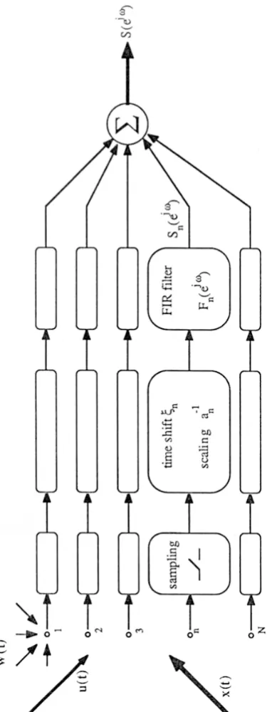
Figure 2.2: Array processing structure for absolutely optimal array filters.

The signalsyn(t) are passed through filtersFn(ω) and summed (see Figure 2.2) to give

S(ω) = N

X

n=1

Fn(ω)X(ω) + N

X

n=1

αne−jωτnFn(ω)U(ω) . (2.13)

In this description, the response of the array to the desired signal is denoted

D(ω) i.e.

D(ω) = N

X

n=1

Fn(ω) (2.14)

while the response of the array to the coherent interference is given as

R(ω) = N

X

n=1

(58)

where

Rn(ω) =αne−jωτnFn(ω) (2.16) In [40], a problem formulation based on minimisingkR(ω)k2_{gave an}

underde-termined system of equations. This problem was then avoided by minimising

PN

i=1kR(ω)−Ri(ω)k2 instead. Note however that there is no guarantee that minimising the difference between each individual filter response and the

overall filtering response will necessarily attenuate the interference response.

However, examples were presented in [40] demonstrating such effect. The

dif-ficulties of [40] in minimisingkR(ω)k2 _{were solved in [41] by generalising the}

cost function using the parameter γ in (2.17). The filter transfer functions22

are adjusted to minimise

J(γ, ω) = 1 2

N

X

n=1

|γR(ω)−(1−γ)Rn(ω)|2 (2.17)

subject to the desired signal all-pass constraint

D(ω) = 1 (2.18)

The filter coefficients for the AOAF are solved in ([41], equation (26) when

γ = 1) as

Fn(ω) =

1/|an|2 −δ(1/a∗n)

PN

m=1(1/am)

PN

m=1(1/|am|2)−δ|PNm=1(1/am)|2

(2.19)

where

δ =N−1 ; an=an(ω) = anejωτn (2.20)

22_Setting _γ _{= 1}_/_{2 corresponds to what was initially called ‘Optimum Array Filters’,}

and settingγ = 1 corresponds to minimisation ofkR(ω)k2 _{giving what was then termed}

Optimal array filtering for seismic inversion