Power quality improvement using a STATCOM inverter

(1)

University of Southern Queensland

Faculty of Health, Engineering and Sciences

Power Quality Improvement Using a STATCOM

Inverter

A dissertation submitted by

Phillip Nicholson

in fulfilment of the requirements of

ENG4111 and ENG4112 Research Project

towards the degree of

Bachelor of Engineering (Honours)

Power Engineering

(2)

ABSTRACT

Most loads on an electrical network are reactive and have a lagging power factor,

this reactive power is mostly supplied from the electricity generators and needs to

be transmitted through the network just like any other load. The transmission of this

reactive power also increases losses and causes unnecessary heating in

infrastructure.

An increase in Photovoltaic (PV) penetration in an electrical system has imposed

several Power Quality (PQ) and voltage stability issues, the intermittent nature of

solar generation mean there is a variable output of power to the system which leads

to power imbalance issues and voltage sags and swells. A solution to this may in

fact lie in the problem, there is a potential for the installed inverters associated with

these systems to be utilised to improve local power quality by supplying or

absorbing reactive power, day or night. Currently inverters are only being utilised

during daylight hours, leaving an expensive piece of equipment lying dormant for

the majority of a day.

This research outlines the gathering of relevant information, compiles a feasibility

assessment and documents expected outcomes and benefits. A research

methodology is provided together with a risk assessment, project schedule and

quality assurance plan and timeline.

This research will provide useful information into the feasibility of grid controlled

Static Compensator (STATCOM) inverters and the benefits this would have on

(3)

University of Southern Queensland

Faculty of Health, Engineering and Sciences

ENG4111 and ENG4112 Research Project

Limitations of Use

The Council of the University of Southern Queensland, its Faculty of Health,

Engineering and Sciences, and the staff of the University of Southern Queensland,

do not accept any responsibility for the truth, accuracy or completeness of material

contained within or associated with this dissertation.

Persons using all or any part of this material do so at their own risk, and not at the

risk of the Council of the University of Southern Queensland, its Faculty of Health,

Engineering and Sciences or the staff of the University of Southern Queensland.

This dissertation reports an educational exercise and has no purpose or validity

beyond this exercise. The sole purpose of the course pair entitles “Research Project”

is to contribute to the overall education within the student’s chosen degree program.

This document, the associated hardware, software, drawings, and any other material

set out in the associated appendices should not be used for any other purpose: if

(4)

CERTIFICATION

I certify that the ideas, designs and experimental work, results, analyses and

conclusions set out in this dissertation are entirely my own effort, except where

otherwise indicated and acknowledged.

I further certify that the work is original and has not been previously submitted for

assessment in any other course or institution, except where specifically stated.

Name: Phillip Nicholson

Student Number: 61040542

Date: 4th October, 2016

__________________________________

(5)

ACKNOWLEDGEMENT

This research project would not have been possible without the assistance of Dr Les

Bowtell. The topic was chosen with guidance from Les after discussions

surrounding my interest in renewable energy and a more efficient future. Les’

involvement in the project included assisting in the research and dissecting results

from the field survey. He suggested areas that required further investigation and

improvements to my site surveying technique. I thank Les sincerely for his

encouraging guidance, friendly advice and generous time donated to me throughout

this project.

I would also like to thank my family, especially my wife and daughter, thank you

for encouraging me in all of my pursuits and inspiring me to complete this degree.

I always knew that you believed in me, you have been my inspiration I needed

(6)

CHAPTER 3 ... 15

RESEARCH AND TEST METHODOLOGY ... 15

3.1 PQ Survey Sites ... 15

3.2 Contingency Plan for PQ Survey ... 16

3.3 PQ Survey ... 16

3.3.1 PQ Meter ... 16

3.3.2 Meter Installation / Recovery Procedure ... 17

3.3.3 Meter Configuration Settings ... 18

3.3.4 Event Trigger Settings ... 19

3.4 Bureau of Meteorology Information ... 20

(8)

3.5.1 Industrial System Model Calculations ... 23

3.5.2 Commercial System Model Calculations ... 24

3.5.3 Residential Rural System Model ... 25

3.6 Power Flow Analysis in MATLAB ... 26

3.7 Risk Assessment ... 28

3.7.1 PQ Survey Risks ... 29

3.7.2 PQ Survey Data Risks ... 29

3.7.3 MATLAB Simulation Risks ... 30

CHAPTER 4 ... 31

DATA AND RESULTS ANALYSIS ... 31

4.1 STATCOM on a Single Bus During Normal Conditions ... 31

4.1.1 Industrial Modelled Systems during Peak Load ... 32

4.1.2 Industrial Modelled Systems during Off-Peak Load ... 34

4.1.3 Commercial Modelled Systems Peak Load ... 36

4.1.4 Commercial Modelled Systems Off-Peak Load ... 38

4.1.5 Residential Modelled Systems during Peak Load ... 40

4.1.6 Residential Modelled Systems during Off-Peak Load ... 42

4.2 STATCOM on a Single Bus During Transient Conditions ... 44

CHAPTER 5 ... 48

DISCUSSION AND IMPLICATIONS ... 48

5.1 STATCOM used for Power Factor Improvement ... 48

5.1.1 Power Factor During Transients ... 49

5.2 STATCOM used for Full Voltage Regulation ... 49

5.2.1 Voltage Regulation During Transients ... 50

(9)

5.5 STATCOM Active and Reactive Power Supply ... 51

CHAPTER 6 ... 53

CONCLUSIONS ... 53

6.1 PQ Improvements using a STATCOM Inverter ... 53

6.2 Future Research ... 54

6.2.1 Investigate feeder with High PV Penetration and VR Issues ... 54

6.2.2 Communication between SMART Meter and SMART Grid ... 55

6.2.3 Review of Current Standards for Inverters ... 55

REFERENCES ... 56

APPENDICES ... 60

Appendix A - Project Specification ... 60

Appendix B - Project Risk Assessment ... 62

Appendix C - Project Timeline ... 65

Appendix D - Resource Requirements ... 69

Appendix E - MATLAB Programs ... 72

Appendix F - Hazard Assessment Check Forms ... 80

Appendix G - PQ Survey Data ... 84

(10)

LIST OF FIGURES

Figure 2.1 Principle Operation of a STATCOM (Yohan Fajar Sidik, 2012) ... 8

Figure 2.2 Grid-Tied PV System with Battery Storage (Solar 2016) ... 11

Figure 2.3 Typical PV System Generation (University 2016) ... 12

Figure 2.4 ITI Curve ((ITI) 2000) ... 13

Figure 3.1 PQ-Box 100 network analyser used to survey selected sites ... 17

Figure 3.2 PQ Meter installed at Manly on transformer cabling ... 18

Figure 3.3 PQ Meter Setup for Basic Settings ... 19

Figure 3.4 PQ Meter Event Trigger Settings ... 20

Figure 3.5 Radial System Model Used for all Load Profiles ... 21

Figure 3.6 Dynamic Load Profiles for SDG&E (Anders 2015) ... 22

Figure 4.1 Industrial Models Bus Voltages during Peak Load ... 33

Figure 4.2 Industrial Models Power Factor during Peak Load ... 34

Figure 4.3 Industrial Models Bus Voltages during Off-Peak Load ... 35

Figure 4.4 Industrial Models Power Factor during Off-Peak Load ... 36

Figure 4.5 Commercial Models Bus Voltages during Peak Load ... 37

Figure 4.6 Commercial Models Power Factor during Peak Load ... 38

Figure 4.7 Commercial Models Bus Voltages during Off-Peak Load ... 39

Figure 4.8 Commercial Models Power Factor during Off-Peak Load ... 40

(11)

Figure 4.11 Residential Models Bus Voltages during Off-Peak Load ... 43

Figure 4.12 Residential Models Power Factor during Off-Peak Load ... 44

Figure 4.13 Industrial Model Bus Voltage during Transient Condition ... 46

Figure 4.14 Industrial Model Power Factor during Transient Condition ... 47

Figure 5.1 STATCOM Size Required for Full Voltage Regulation at Bus 4 ... 50

Figure G-1 Real Power Consumption at Atarmon Site ... 84

Figure G-2 Reactive Power Consumption at Artarmon Site ... 85

Figure G-3 Real Power Consumption for Manly High-rise ... 86

(12)

LIST OF TABLES

Table 3.1 TX and Line Data for Industrial System Model ... 24

Table 3.2 TX and Line Data for Commercial System Model ... 24

Table 3.3 TX and Line Data for Rural System Model ... 25

Table 4.1 Industrial Model Bus and Load Data during Peak Load ... 33

Table 4.2 Industrial Model Bus and Load Data during Off-Peak Load ... 35

Table 4.3 Commercial Model Bus and Load Data during Peak Load ... 37

Table 4.4 Commercial Model Bus and Load Data during Off-Peak Load ... 39

Table 4.5 Residential Model Bus and Load Data during Peak Load ... 41

Table 4.6 Residential Model Bus and Load Data during Off-Peak Load ... 43

Table 4.7 Industrial Model Bus and Load Data during Transient Conditions ... 46

Table B-1 Personal Risk Matrix - Be Safe Pro 10 Managing WHS ... 62

Table B-2 Personal Risk Assessment ... 63

Table B-3 Project Risk Assessment ... 64

Table C-1 Project Timeline ... 66

Table D-1 Project Resources ... 69

Table D-2 Project Resources ... 70

(13)

NOMENCLATURE

The following abbreviations have been used throughout the text: -

PV DC AC CT

STATCOM FACTS PQ PLCC PLN THD VSI Hz VAr VSC TX LV HV USQ

Photovoltaic

Direct Current

Alternating Current

Current Transformer

Static Compensator

Flexible Alternating Current Transmission System

Power Quality

Power Line Communication

Power Line Networking

Total Harmonic Distortion

Voltage Source Inverter

Hertz

Reactive Power

Voltage Source Converter

Transformer

Low Voltage

High Voltage

(14)

INTRODUCTION

1.1

Outline of the Study

There is a need to become more efficient with our energy usage, this includes not

only reducing energy demand, but improving the way in which energy is being

delivered. This study is an ongoing look at the feasibility of converting existing

solar system inverters to STATCOMs. Under the proposal the local energy

requirements would not only be supplied by a customer’s solar system, but could

also help improve the PQ of surrounding electrical installations.

The broader study will investigate the impact of converting an installed inverter, or

replacing a near end of life inverter with a STATCOM, and what benefits that will

have to not only the local installation, but also upstream and downstream customers

as well as the electricity distributor. A STATCOM is a voltage source converter

made up of power electronics, it is currently used on large installations for power

factor correction, and on electricity grids for voltage regulation (VR). A

STATCOM has the added benefit of being able to rapidly respond to changes in PQ

and rectify them within their rated capacity.

1.2

Background

1.2.1Solar Energy

The potential for future shortages of fossil-fuel sources of electric power has led to

the development of the technology needed to use non-polluting renewable fuel

sources such as the sun, wind, and fuel cells (Kirawanich & O'Connell 2000).

(15)

voltage; this can then be converted into an Alternating Current (AC) voltage via the

means of an inverter so it can be used in parallel with the electricity grid.

1.2.2STATCOM

A STATCOM invertor is a Flexible Alternating Current Transmission System

(FACTS), it is used to control the power flow through an electrical transmission

line (Sen 1999). By absorbing and supplying reactive power the STATCOM can

control the power factor of a local load by altering the phase angle of the current in

relation to the voltage. The STATCOM can either be connected directly to the

generation source or can be used through a storage device such as a battery. Many

of these devices are active during the day but often lay dormant during the night

time when there is no sunlight. The ideal output of a STATCOM would be a pure

sinusoidal AC waveform, but this is not possible even with the most advanced

technology, there still exists a small DC output from the inverter into the grid. There

are limits the electricity distribution authority will allow of this DC output and also

the amount of harmonic distortion.

1.2.3The Problem

There is potential for STATCOM inverters used in Solar PV arrays to improve PQ

at the local premises as well as the local electrical grid. This could be done around

the clock as opposed to the relatively short hours of operation that the inverters are

used now during daylight hours only. As the many of the initial batch of inverters

purchased in Australia circa 2007. Purchased under the federal government PV

rebate scheme, reach their expected life cycles in the next few years, it is a poignant

time to look for smarter alternatives for the estimated 10-20yrs of the installed PV

panels.

The electricity grid’s voltage is dependent on the amount of reactive power that is

needed and hence can be controlled with the inducement or absorption of reactive

(16)

1.3

Project Aim

The aim of this work is to carry out power surveys on a selection of sites that have

a PV array installed. The load survey will include load cycle information as well as

apparent and reactive power readings. Records from the Australian Bureau of

Meteorology on the radiance of the sites will also be used. This will provide the

radiance during the time of the survey at each site, the use of this data will avoid

the need to survey the radiance at the same time as the power survey.

The results from the survey will then be modelled in MATLAB so they can be

simulated with a known accurate simulation of a STATCOM inverter, previously

created by Dr Les Bowtell.

1.4

Project Objective

The specific objectives of this project area: -

1. Conduct a literature review on the STATCOM inverter and their PQ

improvement capabilities. Using the literature review determine if these

capabilities are going to be able to provide a significant improvement to the

PQ at selected premises.

2. Perform a load survey of a commercial and high density residential load.

3. Analyse load data and develop a system model for use in MATLAB.

4. Evaluate the transient capabilities of a STATCOM inverter on the system

loads modelled in MATLAB.

5. Report on the potential benefits that can be expected to both the consumer

and electricity distributor from a locally installed STATCOM.

1.5

Thesis Overview

Chapter 2 of the dissertation contains the literature review which has been carried

(17)

Chapter 3 outlines the methodology that was adopted for completing this project,

whilst Chapter 4 reports the data obtained from the load surveys and the results

from the simulation of the system loads modelled in MATLAB. Chapter 5 contains

the in depth discussion surrounding the results.

Finally, Chapter 6 will provide recommendations and conclusions on the study, as

well as suggestions for future research into the development of this project.

1.6

Summary

As can clearly be seen this project will test the feasibility of converting existing

solar system inverters into STATCOMs for the purpose of supplying reactive power

to improve PQ. There is a clear and present need for this study as we shift more of

our load onto renewable energies and look to becoming more energy efficient. It is

hoped this research will offer an alternative method to solving PQ issues on the

(18)

LITERATURE REVIEW

2.1

Overview

A literature review was undertaken to further develop the idea towards a research

project. The purpose of the review was to gather relevant information about:

 Reactive power effect on voltage regulation  Control of STATCOM’s reactive power  Power Quality

 SMART meters

 Grid connected PV systems with battery storage  ITI Curve

The literature review is provided as Appendix A, the following is a brief summary

of the more important points. The review is expected to be continuously revised

throughout the length of the project.

2.2

Reactive Powers Effect on Voltage Regulation

A study by Petoussis (Petoussis et al. 2006) has found that the presence of reactive

power in the network has a significant impact on the electricity market equilibrium

and the power distribution in the network. Reactive power and voltage control is

one of the ancillary services used to maintain the voltage profile through injecting

or absorbing reactive power (Dapu et al. 2005).

If the voltage on a system is too low it will not be able to supply active power, thus

(19)

increase losses. During times of high load there is a drop in voltage in the network,

as the voltage drops there is an increase in current to maintain the amount of power

supplied. This causes the system to absorb more reactive power and thus the voltage

drops even further potentially creating a cascading effect until voltage failure.

2.3

Reactive Power Control in a Distribution Network

There are a number of ways reactive power can be controlled in a distribution

network, some with static control equipment and some dynamic. Examples of the

more common control will be discussed in this review.

2.3.1Generators

An electric generators main function is to convert energy into electric power, this

output power can be considered in terms of their terminal voltage and their reactive

power output. Reactive power is produced by increasing the magnetic field in the

generator by increasing the current in the rotating field winding. Production of

reactive power limits a generators real-power production and so ideally it would be

desirable to be kept to a minimum.

2.3.2Reactors and Capacitor Banks

Electricity distributors install reactors and capacitor banks at the local zone

substations to assist with the generation and absorption of reactive power for the

local area. A capacitor bank will produce reactive power at times of high load where

the voltage in the system has dropped. A reactor will absorb reactive power when

the network voltage is high, normally during low load periods such as the late

evening to early morning. They are both passive devices and as such need to be

switched on and off, usually after the network voltage has reached a set limit away

(20)

2.3.3Static Compensator (STATCOM)

A Static Compensator (STATCOM) is a device that can provide reactive support to

a bus. It consists of a voltage sourced converters connected to an energy storage

device on one side and to the power system on the other (Rao, Crow & Yang 2000).

It is a power electronics device, consisting of insulated-gate bipolar transistor’s

(IGBT) which have a high efficiency and fast switching. Currently they are used on

the electricity grid by the distributor, or as part of large commercial installations for

power factor correction.

2.4

Control of STATCOM’s Reactive Power Output

Studies from Escobar (Escobar, Stankovic & Mattavelli 2000) has found that

STATCOM’s offer several advantages over conventional thyristor-based

convertors solutions for voltage control due to that speed of response, flicker

compensation, flexibility, and minimal interaction with the supply grid.

The output of the STATCOM’s power can be controlled by adjusting the phase

angle between the voltage and current, this is shown in Figure 2.1. If a leading phase

angle is needed then reactive power will be absorbed by the STATCOM by,

however if a lagging phase angle is applied then the STATCOM will produce

reactive power. This control of the STATCOM can be carried out by using a VAr

controller. This VAr controller can be installed locally to the STATCOM to assist

with improving the power factor of the local load by supplying or absorbing reactive

power as needed. The VAr controller can be implemented with the use of logic

(21)

[image:21.595.99.501.73.379.2]

Figure 2.1 Principle Operation of a STATCOM (Yohan Fajar Sidik, 2012)

2.5

Power Quality

The term PQ has been used to describe the variation of the voltage, current, and

frequency on the power system (Reid 1994). Maintaining PQ on an electrical

system refers to maintaining a near perfect sinusoidal waveform of voltage and

current. Many factors on an electrical system can alter and distort these waveforms

including, harmonics, unbalanced loads, transformer vibration and noise. Harmonic

distortion of the power waveform occurs when the fundamental, second, third and

other harmonics are combined. The result is voltage and current contaminations on

the sinusoidal waveform (Henderson & Rose 1993). Poor PQ on a system can lead

(22)

2.6

Smart Meters

SMART meters will play a very important role in the future with customers having

an increased interest in how much energy they used and when. The old disc meters

were only able to give limited energy usage information such as how much was

used, and an indication of how much was being used currently was only possible

by seeing how fast the disc was spinning. The advent of the SMART meter allows

energy companies to charge in a tariff known as time of use, where energy can be

charged at different amounts depending on what time of the day it is being

consumed.

The increase in embedded generation has also seen an increase in SMART meters

as these meters are required for such generation as they allow for a bidirectional

energy flow between the grid and the consumer.

Communication with the SMART meter can be done in a variety of ways, the three

most common ways that have been reviewed by Ali (Ali, Maroof & Hanif 2010)

are:

 RS-232 As Local transmission medium  PLCC Using main power line

 Short Messaging Service on GSM

Power line communication (PLCC) or Power line networking (PLN) which utilises

the same wired medium through which power is delivered to the customer as a

communication channel (Ali, Maroof & Hanif 2010). This is the medium that will

(23)

2.7

Grid connected PV systems with battery storage

Junbiao (Junbiao et al. 2012) states that the integration of PV generation brings

numerous challenges to the system operators and designers such as:

 Changing solar irradiance profile.

 Remote location of PV due to solar energy.

 Inability to meet expected energy output levels without storage or auxiliary

device.

Active power can be balanced by STATCOM with battery storage when battery is

charged when system voltage is higher than upper set value, and discharged when

system voltage is lower than lower set value (Junbiao et al. 2012).

It is expected that as the manufacturing costs of battery storage comes down there

will be an increased uptake of this energy storage at the consumer level. With the

increase of battery storage there is real potential for power factor correction to be

carried out locally rather that via large reactors and capacitor banks that are

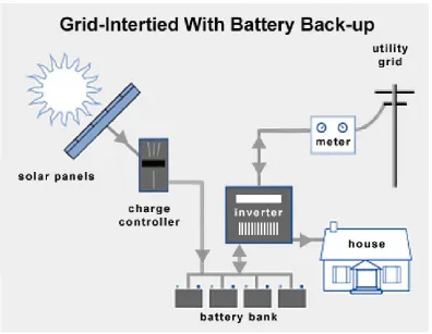
currently operated and maintained by the electricity distributors. Figure 2.2

represents a typical grid-tied PV system on a household with battery storage. The

sun’s energy is converted into DC which is either stored in the battery or converted

(24)

[image:24.595.102.499.69.376.2]

Figure 2.2 Grid-Tied PV System with Battery Storage (Solar 2016)

2.7.1PV Impacts on PQ

The increasing penetration of PV systems on the Low Voltage (LV) network is

creating several PQ and voltage stability issues. The electricity distributor has to

maintain the PQ for all situations, this is becoming increasing difficult due to the

time that PV systems are operating. On a residential load, they are at their peak load

in the evening when there is no sunlight and no PV generation, this would bring

voltages down to their lowest limit. During the day the loads are low by comparison,

but there is also daylight and hence PV generation, this decreases load on the system

and increases voltages. The difference between the high daytime voltage and low

evening voltage becomes larger when there is a higher penetration of PV. Single

phase PV systems also contribute to PQ issues, by suppressing the load on just one

(25)

2.7.2Intermittency of PV Systems

PV systems by nature rely on sunlight to produce energy, the amount of energy

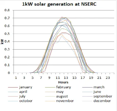
produced varies over the day depending on the amount of solar radiance. Figure 2.3

shows the typical profile of PV generation throughout the day, with the maximum

being generated in the middle of the day, and no generation during the night time.

Throughout the year the amount of energy being generated varies for each month

as the earth transitions through its seasons and the distance from the sun increases

and decreases. A major problem with this type of resource is the variable output

power and limited predictability results in intermittent generation (Chidurala, Saha

& Mithulananthan 2013), this can be caused by large clouds blocking the amount

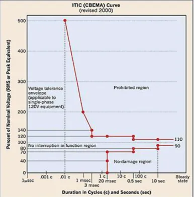
[image:25.595.101.499.347.723.2]

(26)

2.8

ITI (CBEMA) Curve

The ITI, formerly CBEMA, curve was developed by the Information Technology

Industry Council of the United States of America(USA) (Elphick & Smith 2010).

The curve attempts to shows the voltages that can be tolerated by Information

Technology (IT) equipment without causing damage or interruption. Whilst the

curve has been developed for the USA and their 120 V nominal voltage, the curve

with its percentage of nominal voltage on the y-axis can be translated into the

[image:26.595.101.490.280.673.2]

Australian 230 V standard, a copy of the curve can be seen in Figure 2.4.

(27)

The x-axis represents the time spent in that range. There are two prohibited regions

on the curve, the upper region is for over voltages and will likely cause damage to

IT equipment. The lower region is for under voltages and whilst it is unlikely it will

cause damage to electronic equipment it will tend to cause interruptions.

2.9

Voltage Control

On an AC system voltage control is managed by absorbing and producing reactive

power. Managing reactive power in this way in affect changes the phase shift

between the current and the supply voltage, producing reactive power will have a

capacitive effect and will cause a leading power factor, whereas absorbing reactive

power will have an inductive effect and cause a lagging power factor. Tanaka

(Tanaka et al. 2009) states that reactive power control has a possibility to contribute

for reduction of distribution loss. In 2011 the Australian Standards PQ Committee

published AS 61000.3.100-2011 (Standards 2011), this defines that the voltage at a

premises needs to be within the rage of 230 V +10% or -6%. The further away from

a transformer (TX) a supply is generally means the lower their supply voltage will

be. This problem is worsened during periods of high load, which for residential

loads tends to be in the early evening.

2.10

Review of Information

It is clear from the literature review that using a STATCOM inverter to improve

power factor is efficient and has a fast response, which will be ideal in the scope of

this project as the power factor will be read in real time from the SMART meter.

The STATCOM will act as either capacitor or inductor as it is instructed to absorb

or produce reactive power when improving power factor. Communication with the

SMART meter will be carried out using Power Line Communication which will

negate the need for extra wiring.

Further review will be required throughout the project to improve knowledge in

(28)

RESEARCH AND TEST METHODOLOGY

3.1

PQ Survey Sites

PQ surveys were collected from various sites around the Northern Sydney region

during the Autumn and Winter months in 2016. Targeted sites for the survey were

either a medium density apartment block or a mix commercial and residential

property needing to have a solar PV array installed. A variety of sites were initially

chosen and PV arrays confirmed using the high resolution aerial imagery service

from nearmaps. Only two sites, one of each load profile was required so the list was

narrowed down to sites with a supply from above ground substations to facilitate

an easier and safer installation of the PQ meter. The measurement device was

installed and left capturing for the same length of time. Sites chosen for the survey

were:

 High-rise Building in Manly – Mixed residential and commercial load  Apartment Block in Artarmon – Residential load

Unfortunately, time did not permit the survey of an industrial factory and previous

surveys carried out were not set at a suitable time interval for this projects

requirements. At each of the above sites their load was surveyed over a period of

one week. Although due to the finite amount of internal memory in the PQ meter a

whole week was sometimes not possible to be captured depending on how many

events were captured. The PQ meter was installed at the supplying substation of the

load. Ideally the meters would have been best installed on the terminals of the

customer’s main switchboard, but access to these terminals was not possible due to

security metering tags clipped onto the protective covers preventing unauthorized

(29)

3.2

Contingency Plan for PQ Survey

If the required measurement devices are not available for use on my project, or the

data I obtain from the survey is corrupt or unusable, a contingency plan was devised.

Numerous surveys are carried out as part of the distributor’s Low Voltage Network

PQ Survey every year to ensure that suitable conditions provided to customers in

terms of voltage ranges, voltage fluctuations, and voltage harmonics etc. are being

adhered to. It was decided that in the event a survey specifically carried out for this

project was unable to occur, two surveys previously carried out on suitable sites

would be obtained from the distributor with permission and used as part of this

research project.

3.3

PQ Survey

All survey work was carried out around Northern Sydney during the second quarter

of 2016. Measuring equipment and software to download the data was provided by

the company, as was the person protective equipment used when installing and

recovering the metering equipment. Risk assessments were carried out for the

hazardous work and copies can be found in Appendix B -. Pre work hazard

assessment checks were also carried out before any works, these can be found in

Appendix F -.

3.3.1PQ Meter

In this survey the sites were each monitored for one week by a high end PQ meter

for a range of PQ parameters including Current, Voltage, Energy (P, Q, P+, P-, Q+,

Q-), Harmonics & Total Harmonic Distortion (THD), Voltage Fluctuations

(Flicker) and Frequency. The measurement device used for the survey was a

PQ-Box 100 Network Analyser, shown in Figure 3.1. This meter is suitable for low,

medium and high-voltage networks. The meter has annual calibration and was

(30)

[image:30.595.143.453.71.482.2]

Figure 3.1 PQ-Box 100 network analyser used to survey selected sites

3.3.2Meter Installation / Recovery Procedure

The PQ meters were installed at the supplying substations. Sites were selected

ensuring that they had a direct distributor supplying them so that only the load of

the site would be surveyed. In the case of the High Rise Building in Manly the

supply was from a firm rated two TX chamber substation. Due to the size of the

consumer mains the current transformers (CTs) had to be installed around the

cabling from one of the TXs, shown in Figure 3.2. There were LV bus links on the

(31)

[image:31.595.101.497.69.329.2]

Figure 3.2 PQ Meter installed at Manly on transformer cabling

The other site was supplied via a direct distributor from a ground kiosk. The direct

distributor was a multicore cable but the CTs were able to be installed around each

core separately inside the kiosk underneath the LV board. The voltage clamps were

also installed at the kiosk on the distributor.

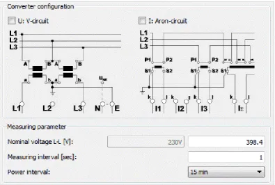
3.3.3Meter Configuration Settings

The meter was set up for a 50 Hz 4 wire system with a nominal voltage of 230 V

phase to neutral and 398.4 V phase to phase. The measuring interval was set to 1

second which was the fastest setting, to get the most accurate and true reading. Flexi

current TXs were placed around each distributors cables including the neutral, and

voltage clamps were placed on the exposed terminations at the substation for each

phase of the distributor and neutral. The basic settings for the PQ meter are shown

(32)

[image:32.595.101.497.71.337.2]

Figure 3.3 PQ Meter Setup for Basic Settings

3.3.4Event Trigger Settings

The event trigger function of the meter was set to capture any voltage variations

outside the configurable thresholds, configuration used to show in Figure 3.4 In the

event the voltage went outside the thresholds the meter would start recording at

intervals of 10ms with a pre event record time of 1000ms and a total record time of

3000ms. For this survey the lower threshold was set to 90% of RMS, and the upper

threshold to 110% of RMS. These limits were chosen as operating outside these

limits may cause damage to customer’s electrical equipment as shown in the ITI

(33)

Figure 3.4 PQ Meter Event Trigger Settings

3.4

Bureau of Meteorology Information

The daily solar exposure information was obtained from the Australian Government

Bureau of Meteorology (BOM) website. This data is from a computer model that is

run by the BOM and produces an estimate of the total amount of solar radiation that

reaches the earth on a given day.

3.5

Development of the System Model

A model of a radial electrical system was developed and used to study the transient

capabilities a STATCOM inverter would have on the system loads, shown in Figure

3.5. The data from the power surveys was used to produce typical radial systems in

a suburban area. The models have one large generator, one transmission line going

to a zone TX feeding one high voltage feeder. The feeder is supplying four Load

(34)

capabilities. This is so the effects could be seen not only at the localised load, but

also for the upstream and downstream loads.

Figure 3.5 Radial System Model Used for all Load Profiles

Three models have been made up to represent different load profiles that are

commonly found on an electrical network. These include an industrial load model,

(35)

during the business hours of the day and the residential loads having a small peak

in the morning and a larger peak in the evening once residents have returned home

from work.

Figure 3.6 Dynamic Load Profiles for SDG&E (Anders 2015)

All models have the same radial setup as shown in Figure 3.5, but will have different

Bus and Line data as well as different loading. Each models data will be discussed

in more detail later. For the data to be used in MATLAB all the values needed to

be Per Unit values. In order to use the per unit method we had to normalise all the

system impedances to a common base. Any values that were sourced from data

(36)

The following selections were made for per unit calculations:

𝑆_{𝑏𝑎𝑠𝑒} = 20 𝑀𝑉𝐴

𝑉𝑏𝑎𝑠𝑒= 11 𝑘𝑉

𝐼_{𝑏𝑎𝑠𝑒} = 𝑆𝑏𝑎𝑠𝑒 𝑉_{𝑏𝑎𝑠𝑒}√3=

20

11 × √3= 1.050 𝑘𝐴

𝑍𝑏𝑎𝑠𝑒 =

𝑉𝑏𝑎𝑠𝑒

𝐼_{𝑏𝑎𝑠𝑒}√3=

11

1.050 × √3= 6.048 Ω

𝑌𝑏𝑎𝑠𝑒 =

1 𝑍𝑏𝑎𝑠𝑒

= 1

6.048= 0.165 𝑆

The zone TX is a 20 MVA TX (33/11 kV) with 6% impedance at 100 MVA, this

needs to be converted to the 20 MVA base.

𝑍_𝑇𝑥1% = 6% ×𝑆𝑛𝑒𝑤𝑏𝑎𝑠𝑒

𝑆_{𝑜𝑙𝑑𝑏𝑎𝑠𝑒} = 6% × 20

100= 1.2%

∴ 𝑍_{𝑝𝑢 𝑇𝑥1} = 𝑆𝑏𝑎𝑠𝑒 𝑆_𝑇𝑥1 ×

𝑍_𝑇𝑥1 100 =

20 20×

1.2

100= 0.012 𝑝𝑢

3.5.1Industrial System Model Calculations

The industrial model was designed around a typical feeder layout found in an

industrial area around Northern Sydney. It is an underground feeder which has been

direct laid using 11kV 300 AL3 P H L SW J cable. The cable has an impedance of

0.094 + j0.069 Ohms/km, and a Susceptance of 0.251 mS/km. For simplicity the

distance between each bus has been taken at an average of 600 metres. This gives

(37)

segments of the feeder. All line and TX data can be seen in Table 3.1,and has been

converted into per unit values.

Table 3.1 TX and Line Data for Industrial System Model

TX / Line Number

Impedance p.u.

Susceptance p.u. TX 1 0.005 + j0.012

Line 1 0.009 + j0.007 j0.0009

Line 2 0.009 + j0.007 j0.0009

Line 3 0.009 + j0.007 j0.0009

The loading on each of the buses was based off the power surveys carried out, for

the industrial load profile it was found to have a peak during the day between

normal working hours, and relatively low load was seen over night. The values for

loads can be seen later on in CHAPTER 4.

3.5.2Commercial System Model Calculations

The commercial model was designed around a typical feeder layout found in a

commercial area such as that of North Sydney, predominantly made up of

commercial high rise buildings with little residential loading. Like the industrial

area the it has been modelled off an underground feeder, but due to the density of

the high-rises the distance between each bus has been reduced to 400 metres. This

gives an impedance of 0.038 + j0.028 Ohms, and a susceptance of 0.1004 mS for

all segments of the model. All line and TX data can be seen in Table 3.2, and has

been converted to per unit values.

Table 3.2 TX and Line Data for Commercial System Model

TX / Line Number

Impedance p.u.

Susceptance p.u.

TX 1 0.005 + j0.012

Line 1 0.006 + j0.005 j0.0006

Line 2 0.006 + j0.005 j0.0006

(38)

From the power survey data, it was showed that the loading for the commercial

profile was found to be similar to that of the industrial load profile, with its peak

occurring during normal working hours of the day, and a relatively low load in the

evening.

3.5.3Residential Rural System Model

The rural model was designed around a typical feeder layout found in a rural area

with residential load such as that of North West Sydney around Berowra. On rural

lines the feeder is predominantly made up of long overhead lines feeding pole top

TXs. The distance between the buses has been increased due to the geographical

nature of a rural line and residences being further apart, the average line distance

has been taken as 800 metres. Whilst this distance is longer than the underground

models it is considered a short length line in terms of overhead lines, as such the

shunt admittance and therefore line susceptance can be neglected for short lines. A

typical cable used in rural areas is 66 CDCU3, this has an impedance of 0.338 +

j0.371 Ohms/km, with the average length of 800 metres this gives an impedance of

0.270 + j0.297 Ohms for each line segment.

Table 3.3 TX and Line Data for Rural System Model

TX / Line Number

Impedance p.u.

Susceptance p.u.

TX 1 0.005 + j0.012

Line 1 0.045 + j0.049 NA

Line 2 0.045 + j0.049 NA

Line 3 0.045 + j0.049 NA

The residential load profile data obtained from the power survey showed that there

was a small peak for load in the morning, when people woke and got ready to go to

work, and another in the early evening when they arrived home and proceeded to

get dinner ready. During the day the load was low, but it was lowest overnight

(39)

3.6

Power Flow Analysis in MATLAB

To solve the power flow problem in the model the Newton-Raphson method will

be used, calculated using MATLAB. The idea behind the method is that an initial

estimate of the root of the function is made. From that estimate a tangent line is

computed and the x-intercept of this tangent is found, this new root value is checked

against the initial estimate and in most cases will be a better approximation to the

functions root. Using the new approximation, the process is repeated until

convergence.

When the Newton-Raphson method is applied to power flow problems it is being

used to solve the bus voltage magnitudes and angles. The swing bus or slack bus is

the only bus which the voltage is known and specified. In the model developed the

swing bus is G1 which is the generator bus. The voltages are estimated for all other

buses, and their real power (P) and reactive power (Q) are entered. For this model

P and Q were surveyed for one of the buses (Bus 5) and all others have been chosen

from typical loads found on a suburban feeder.

Each non slack bus of the system will have two unknowns, voltage (Vi) and angle

(δi), and two knowns Pi and Qi. If we collect all the mismatched equations into

(40)

[ 𝛿𝑃₂ 𝛿𝛿2

⋯ 𝛿𝑃5 𝛿𝛿5

⋮ 𝐽₁₁ ⋮ 𝛿𝑃₄

𝛿𝛿2

… 𝛿𝑃5 𝛿𝛿5

| |

|𝑉2|

𝛿𝑃₂ 𝛿|𝑉2|

⋯ |𝑉5|

𝛿𝑃₂ 𝛿|𝑉5|

⋮ 𝐽₁₂ ⋮

|𝑉2|

𝛿𝑃₅ 𝛿|𝑉2|

⋯ |𝑉5|

𝛿𝑃₅ 𝛿|𝑉5|

𝛿𝑄₂ 𝛿𝛿₂ ⋯

𝛿𝑄₅ 𝛿𝛿₅ ⋮ 𝐽₂₁ ⋮ 𝛿𝑄4

𝛿𝛿₂ … 𝛿𝑄5 𝛿𝛿₅ ̅̅̅̅̅̅̅̅̅̅̅̅̅̅̅̅̅̅̅̅ | | | | | ||𝑉2|

𝛿𝑄₂

𝛿|𝑉₂| ⋯ |𝑉5| 𝛿𝑄₂ 𝛿|𝑉₅|

⋮ 𝐽₂₂ ⋮

|𝑉2|

𝛿𝑄5

𝛿|𝑉₂| ⋯ |𝑉5| 𝛿𝑄5

𝛿|𝑉₅| ̅̅̅̅̅̅̅̅̅̅̅̅̅̅̅̅̅̅̅̅̅̅̅̅̅̅̅̅̅̅̅̅̅̅ ] ⏟ 𝐽𝑎𝑐𝑜𝑏𝑖𝑎𝑛 [ ∆𝛿₂ ⋮ ∆𝛿₅ ∆|𝑉₂|

|𝑉₂| ⋮

∆|𝑉5|

|𝑉5|

̅̅̅̅̅̅̅ ] ⏟ 𝐶𝑜𝑟𝑟𝑒𝑐𝑡𝑖𝑜𝑛𝑠 = [ ∆𝑃₂ ⋮ ∆𝑃₅ ∆𝑄2 ⋮ ∆𝑄5 ̅̅̅̅̅ ] ⏟ 𝑀𝑖𝑠𝑚𝑎𝑡𝑐ℎ𝑒𝑠

Each element of the submatrix J11 can be found using the following formula:

𝛿𝑃𝑖

𝛿𝛿_𝑗 = −|𝑉𝑖𝑉𝑗𝑌𝑖𝑗| sin(𝜃𝑖𝑗 + 𝛿𝑗− 𝛿𝑖)

With the diagonal elements found using:

𝛿𝑃𝑖

𝛿𝛿_𝑖 = − ∑ 𝛿𝑃𝑖

𝛿𝛿_𝑛

𝑁 𝑛=1

𝑛≠𝑖

= −𝑄_𝑖− |𝑉_𝑖|2_𝐵 𝑖𝑖

In a similar manner the elements of submatrix J21 can be found using the following

formula:

𝛿𝑄_𝑖

𝛿𝛿_𝑗 = −|𝑉𝑖𝑉𝑗𝑌𝑖𝑗| cos(𝜃𝑖𝑗+ 𝛿𝑗− 𝛿𝑖)

(41)

𝛿𝑄𝑖

𝛿𝛿_𝑗 = − ∑ 𝛿𝑄𝑖

𝛿𝛿_𝑛

𝑁 𝑛=1

𝑛≠𝑖

= 𝑃_𝑖 − |𝑉_𝑖|2_𝐺 𝑖𝑖

The elements of submatrix J12 can be found using the following formula:

|𝑉𝑗|

𝛿𝑃_𝑖 𝛿|𝑉𝑗|

= −𝛿𝑄𝑖 𝛿𝛿𝑗

|𝑉_𝑖| 𝛿𝑃𝑖 𝛿|𝑉_𝑖|=

𝛿𝑄_𝑖

𝛿𝛿_𝑖 + 2|𝑉𝑖|

2_𝐺

𝑖𝑖 = 𝑃𝑖 + |𝑉𝑖|2𝐺𝑖𝑖

And finally the elements of submatrix J22 can be found using the following

formula:

|𝑉_𝑗| 𝛿𝑄𝑖 𝛿|𝑉𝑗|

=𝛿𝑃𝑖 𝛿𝛿_𝑗

|𝑉_𝑖| 𝛿𝑄𝑖 𝛿|𝑉_𝑖|= −

𝛿𝑃_𝑖

𝛿𝛿_𝑖 + 2|𝑉𝑖|

2_𝐵

𝑖𝑖 = 𝑄𝑖− |𝑉𝑖|2𝐵𝑖𝑖

3.7

Risk Assessment

This research did involve tasks that had an element of risk to them. Safety of

personal involved in the research and the public was of the utmost importance

during this project and as such a risk assessment was undertaken to minimize the

chance of injury to oneself or others, and damage to equipment. The project

(42)

3.7.1PQ Survey Risks

The first and major risk to be analysed is associated with the PQ Survey. More

specifically the installation and removal of the metering devices for the survey. This

task could only be performed by coming within close proximity to exposed live low

voltage switchgear where the various clips and tongs would need to be installed.

The task could be considered medium risk as it is possible that contact could be

made with exposed LV mains and apparatus. The consequence of the risk could be

anywhere from Moderate to Severe in the worst case scenario and as such a Medium

Risk level was assigned to this task. To control this risk several measures, and as

such correct Personal Protective Equipment was needed to minimise the risk of

accidental contact. Ideally it would have been nest to have the LV switchgear

de-energised during the installation but this would have required an interruption to a

large number of customers so was not done. Further risk mitigation included having

an observer on site during the works who was competent in low voltage release and

rescue in the unlikely chance that contact was made with the live mains. Site

awareness of all live mains and apparatus was documented in a pre-works Hazard

Assessment Check (HAC) to ensure all parties present knew of the risks. The

project risk assessment is summarised in Appendix B, and the Hazard Assessment

Check Forms used during the site surveys can be found in Appendix F -.

3.7.2PQ Survey Data Risks

Whilst these may not result in harm or injury to one’s person, the risk is in relation

to the timely completion on this project. Data obtained from the power surveys shall

be immediately checked against corruption, and if found to be corrupt the site will

need to be resurveyed. Once the data has been validated it shall be stored on the

cloud to minimise the chance that it could be lost due to accidental deletion or a

failed hard drive. This will also ensure that it will be accessible from multiple

(43)

3.7.3MATLAB Simulation Risks

Other foreseeable risks are attributed to the MATLAB simulation portion of the

project. It is possible that the data obtained from the sites may be within the

threshold limits and would record zero threshold events. In this case a lower

threshold will need to be applied post survey using MATLAB software or

equivalent to locate times in the survey of interest. There is also the real chance that

the data will not be able to be read into MATLAB and simulated due to

inexperience. To mitigate this risk a revision of previous learned techniques in

loading external data in to MATLAB shall be refreshed early on in the project

timeline.

Other risk mitigations techniques include using the PQ survey data for load profile

usage only, and using only the maximum and minimum loads observed for

simulation in the model. This will provide theoretical results but not a real world

example. If also no transients are recorded during the time of the surveys, a transient

can be simulated by increasing the required active and reactive load on one of the

buses in the model. This transient would be in relation to a large piece of equipment

(44)

DATA AND RESULTS ANALYSIS

Surveys were carried out at the local substation supplying different load profiles,

one apartment block with residential load, and one high rise with a mixed

commercial and residential load. The surveys ran smoothly and data was logged

correctly, load profiles were obtained over a 5-day period on 2 separate occasions

for each site. The issue with the data lay in the type of loads at each site. The

intention of the survey was to capture data where voltage transients could be seen

rising above the threshold of 110% or falling below 90% of nominal voltage. At

both locations the only instances where voltage dropped outside these ranges was

when there was an interruption to supply from the distributor.

An attempt to get data from a local electricity distributor was undertaken where

voltage transients had been present throughout a power survey, but was

unsuccessful after the contact at the distributor was unavailable to provide data in

the timeline required. The maximum and minimum loads were recorded and will

be used in the model to simulate peak and off-peak demand. Load profiles for an

industrial, commercial and rural system were developed and the following tests

carried out.

4.1

STATCOM on a Single Bus During Normal Conditions

To determine the impact a STATCOM can have on an electrical network, the

STATCOM was installed on a single Bus only. Bus 4 was chosen so that the effects

could be seen on the other Load Buses upstream and downstream of the

STATCOM. To make the results more apparent the same active and reactive loads

were chosen for all of the load Buses in the model. Peak loads and Off-Peak Loads

(45)

Secondly, where the STATCOM is installed on Bus 4 and acting in Power Factor

Correction mode, where the inductive load that is being consumed by Bus 4 is being

supplied from the STATCOM operating in a capacitive manner, these will

theoretically cancel one another out and leave the sum of reactive power for Bus 4

equal to zero. Thirdly, the STATCOM will be operating in VR mode where it will

be exporting excess reactive power to the model to bring the voltage at Bus 4 back

up to 1 p.u.

It must be noted that during simulation the STATCOM was only supplying reactive

power, normally an inverter installed by a customer would be supplying active

power. Australian Standards (Australia 2015) stipulate that an inverter must

maintain a power factor between 0.95 lagging and 0.95 leading. The reasoning for

going beyond this limit was to show what effect this would have on the immediate

customer, surrounding customers, and the electricity grid.

4.1.1Industrial Modelled Systems during Peak Load

In the case where a STATCOM was installed at Bus 4 for Power Factor Correction

the voltage drops from Bus 1 to 4 was reduced by 0.26 %, this is an improvement

of 14.27 %. A reduction can also be seen for the other load buses upstream and

downstream. The power factor was improved to unity for Bus 4, but the remaining

load buses power factor remained unchanged. There was also a change in the power

factor of Bus 1 which improved by 0.062, this is due to the reduced reactive power

generation of 2.03 MVArs.

In the second case where a STATCOM was installed at Bus 4 for full VR there was

no voltage drop between Bus 1 to 4, a very significant improvement can also be

seen at all other load buses. The voltage rise on Bus 2 is due to the leakage reactance

of the TX between Buses 1 and 2. The power factor at Bus 4 however was

dramatically affected by increased exportation of reactive power, and became 0.236

leading. This was left off the graph due to it being so far off scale. The power factors

(46)

Figure 4.1 Industrial Models Bus Voltages during Peak Load

Table 4.1 Industrial Model Bus and Load Data during Peak Load

Bus No. Voltage (p.u.)

Angle Degree

Generation Load MW MVAR MW MVAR

Without STATCOM

1 1.000 0.000 12.140 8.139 0 0

2 0.992 -0.005 0 0 3 2

3 0.986 -0.006 0 0 3 2

4 0.982 -0.006 0 0 3 2

5 0.979 -0.006 0 0 3 2

Power Factor STATCOM

at Bus 4

1 1.000 0.000 12.118 6.109 0 0

2 0.993 -0.006 0 0 3 2

3 0.988 -0.007 0 0 3 2

4 0.984 -0.008 0 2 3 2

5 0.982 -0.008 0 0 3 2

Voltage Regulation

STATCOM at Bus 4

1 1.000 0.000 12.190 -6.183 0 0

2 1.001 -0.009 0 0 3 2

3 0.999 -0.016 0 0 3 2

4 1.000 -0.023 0 14.345 3 2

(47)

Figure 4.2 Industrial Models Power Factor during Peak Load

4.1.2Industrial Modelled Systems during Off-Peak Load

factor of Bus 1 which improved by 0.019, this was due to the reduced reactive

power generation by 0.1 MVars.

seen at all other load buses. The power factor at Bus 4 however was dramatically

(48)

remaining load buses were unchanged. The generator on Bus 1 has started to absorb

reactive power instead of supplying and has a leading power factor of 0.862.

Figure 4.3 Industrial Models Bus Voltages during Off-Peak Load

Table 4.2 Industrial Model Bus and Load Data during Off-Peak Load

Angle Degree

Without STATCOM

1 1.000 0.000 1.201 0.347 0 0 2 0.999 -0.001 0 0 0.3 0.1 3 0.999 -0.001 0 0 0.3 0.1 4 0.999 -0.001 0 0 0.3 0.1 5 0.998 -0.001 0 0 0.3 0.1 Power

Factor STATCOM

at Bus 4

1 1.000 0.000 1.201 0.247 0 0 2 1.000 -0.001 0 0 0.3 0.1 3 0.999 -0.001 0 0 0.3 0.1 4 0.999 -0.001 0 0.1 0.3 0.1 5 0.999 -0.001 0 0 0.3 0.1 Voltage

Regulation STATCOM

(49)

Figure 4.4 Industrial Models Power Factor during Off-Peak Load

4.1.3Commercial Modelled Systems Peak Load

power generation of 0.70 MVars.

seen at all other load buses. The power factor at Bus 4 however was dramatically

(50)

remaining load buses were unchanged. The generator on Bus 1 has started to absorb

reactive power instead of supplying and has a leading power factor of 0.885.

Figure 4.5 Commercial Models Bus Voltages during Peak Load

Table 4.3 Commercial Model Bus and Load Data during Peak Load

Angle Degree

Without STATCOM

1 1.000 0.000 6.023 2.799 0 0 2 0.997 -0.003 0 0 1.5 0.7 3 0.995 -0.003 0 0 1.5 0.7 4 0.994 -0.004 0 0 1.5 0.7 5 0.993 -0.004 0 0 1.5 0.7 Power

Factor STATCOM

at Bus 4

1 1.000 0.000 6.021 2.096 0 0 2 0.997 -0.003 0 0 1.5 0.7 3 0.996 -0.004 0 0 1.5 0.7 4 0.994 -0.004 0 0.7 1.5 0.7 5 0.994 -0.004 0 0 1.5 0.7 Voltage

Regulation STATCOM

(51)

Figure 4.6 Commercial Models Power Factor during Peak Load

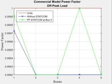
4.1.4Commercial Modelled Systems Off-Peak Load

there was a very slight reduction in the voltage drop from Bus 1 to 4 but this was

less than 0.001% so will be ignored, a reduction can also be seen for the other load

buses upstream and downstream. The power factor was improved to unity for Bus

4, but the remaining load buses power factor remained unchanged. There was also

a change in the power factor of Bus 1 which improved by 0.0002, this was due to

the reduced reactive power generation of 0.02 MVars.

no voltage drop between Bus 1 to 4, an improvement can also be seen at all other

load buses. The power factor at Bus 4 however was dramatically affected by

(52)

load buses were unchanged. The generator on Bus 1 has started to absorb reactive

[image:52.595.100.500.112.415.2]

power instead of supplying and has a leading power factor of 0.858.

Figure 4.7 Commercial Models Bus Voltages during Off-Peak Load

Table 4.4 Commercial Model Bus and Load Data during Off-Peak Load

Angle Degree

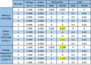
Without STATCOM

1 1.000 0.000 2.002 0.047 0 0 2 0.999 -0.001 0 0 0.5 0.02 3 0.999 -0.002 0 0 0.5 0.02 4 0.999 -0.002 0 0 0.5 0.02 5 0.999 -0.002 0 0 0.5 0.02 Power

Factor STATCOM

at Bus 4

1 1.000 0.000 2.002 0.027 0 0 2 0.999 -0.001 0 0 0.5 0.02 3 0.999 -0.002 0 0 0.5 0.02 4 0.999 -0.002 0 0.02 0.5 0.02 5 0.999 -0.002 0 0 0.5 0.02 Voltage

Regulation STATCOM

[image:52.595.103.495.485.764.2]

(53)

[image:53.595.103.498.76.371.2]

Figure 4.8 Commercial Models Power Factor during Off-Peak Load

4.1.5Residential Modelled Systems during Peak Load

power generation of 0.07 MVars.

(54)

[image:54.595.100.502.126.428.2]

Figure 4.9 Residential Models Bus Voltages during Peak Load

Table 4.5 Residential Model Bus and Load Data during Peak Load

Angle Degree

Without STATCOM

1 1.000 0.000 0.802 0.282 0 0

2 1.000 0.000 0 0 0.2 0.07

3 0.998 -0.001 0 0 0.2 0.07 4 0.997 -0.002 0 0 0.2 0.07 5 0.996 -0.002 0 0 0.2 0.07 Power

Factor STATCOM

at Bus 4

1 1.000 0.000 0.801 0.212 0 0

2 1.000 0.000 0 0 0.2 0.07

3 0.998 -0.002 0 0 0.2 0.07 4 0.997 -0.002 0 0.07 0.2 0.07 5 0.996 -0.003 0 0 0.2 0.07 Voltage

Regulation STATCOM

[image:54.595.102.497.496.761.2]

(55)

[image:55.595.101.499.76.371.2]

Figure 4.10 Residential Models Power Factor during Peak Load

4.1.6Residential Modelled Systems during Off-Peak Load

there was a very slight reduction in the voltage drop from Bus 1 to 4 but this was

less than 0.001% so will be ignored, a reduction can also be seen for the other load

buses upstream and downstream. The power factor was improved to unity for Bus

4, but the remaining load buses power factor remained unchanged. There was also

a change in the power factor of Bus 1 which improved by 0.022, this was due to the

reduced reactive power generation of 0.01 MVars.

(56)

[image:56.595.100.499.112.415.2]

Figure 4.11 Residential Models Bus Voltages during Off-Peak Load

Table 4.6 Residential Model Bus and Load Data during Off-Peak Load

Angle Degree

Without STATCOM

1 1.000 0.000 0.120 0.040 0 0 2 1.000 0.000 0 0 0.03 0.01 3 1.000 0.000 0 0 0.03 0.01 4 0.999 0.000 0 0 0.03 0.01 5 0.999 0.000 0 0 0.03 0.01 Power

Factor STATCOM

at Bus 4

1 1.000 0.000 0.120 0.030 0 0 2 1.000 0.000 0 0 0.03 0.01 3 1.000 0.000 0 0 0.03 0.01 4 1.000 0.000 0 0.01 0.03 0.01 5 0.999 0.000 0 0 0.03 0.01 Voltage

Regulation STATCOM

[image:56.595.100.496.485.763.2]

(57)

[image:57.595.102.500.75.372.2]

Figure 4.12 Residential Models Power Factor during Off-Peak Load

4.2

STATCOM on a Single Bus During Transient Conditions

To determine the effects of a STATCOM connected to a single bus during transient

conditions the same model was used, but the reactive load of Bus 4 was adjusted. It

was apparent after the first lot of simulations for normal conditions that the results

were similar but the magnitude of the reduction or improvements varied with the

loading of the model. Thus only the industrial model during peak load was chosen

for evaluation of the transient due to its well defined difference between all three

scenarios.

The transient load applied to the model was that of a typical induction motor starting

or other heavy plant turning on where a sudden inrush of reactive power is required.

This was only applied to Bus 4 and was taken as 2.5 times the normal reactive load.

(58)

downstream. The power factor was improved to unity for Bus 4, this is a quite

significant improvement of 0.486 from the scenario where no STACOM was

installed. The remaining load buses power factor remained unchanged, but there

was also a change in the power factor of Bus 1 which improved by 0.157, this was

due to the reduced reactive power generation of 5.09 MVars during the transient

condition.

increased exportation of reactive power, and became 0.236 leading. This was left

off the graph due to it being so far off scale. The power factors of the remaining

(59)

[image:59.595.101.500.73.371.2]

Figure 4.13 Industrial Model Bus Voltage during Transient Condition

Table 4.7 Industrial Model Bus and Load Data during Transient Conditions

Angle Degree

Without STATCOM

1 1.000 0.000 12.194 11.203 0 0

2 0.990 -0.005 0 0 3 2

3 0.983 -0.003 0 0 3 2

4 0.978 -0.002 0 0 3 5

5 0.975 -0.002 0 0 3 2

Power Factor STATCOM

at Bus 4

1 1.000 0.000 12.118 6.109 0 0

2 0.993 -0.006 0 0 3 2

3 0.988 -0.007 0 0 3 2

4 0.984 -

Power quality improvement using a STATCOM inverter

University of Southern Queensland

University of Southern Queensland

CERTIFICATION

ACKNOWLEDGEMENT

TABLE OF CONTENTS

1.2.2 STATCOM ... 2

CHAPTER 3 ... 15

CHAPTER 4 ... 31

CHAPTER 5 ... 48

REFERENCES ... 56

LIST OF TABLES

NOMENCLATURE

STATCOM FACTS PQ PLCC PLN THD VSI Hz VAr VSC TX LV HV USQ

INTRODUCTION

Background

1.2.1Solar Energy

1.2.2STATCOM

1.2.3The Problem

Project Aim

Project Objective

Thesis Overview

Summary

LITERATURE REVIEW

Reactive Powers Effect on Voltage Regulation

Reactive Power Control in a Distribution Network

2.3.1Generators

2.3.2Reactors and Capacitor Banks

2.3.3Static Compensator (STATCOM)

Control of STATCOM’s Reactive Power Output

Figure 2.1 Principle Operation of a STATCOM (Yohan Fajar Sidik, 2012)

Power Quality

Smart Meters

Grid connected PV systems with battery storage

Figure 2.2 Grid-Tied PV System with Battery Storage (Solar 2016)

2.7.2Intermittency of PV Systems

ITI (CBEMA) Curve

Voltage Control

Review of Information

RESEARCH AND TEST METHODOLOGY

Contingency Plan for PQ Survey

PQ Survey

3.3.1PQ Meter

Figure 3.1 PQ-Box 100 network analyser used to survey selected sites

Figure 3.2 PQ Meter installed at Manly on transformer cabling

3.3.3Meter Configuration Settings

Figure 3.3 PQ Meter Setup for Basic Settings

Figure 3.4 PQ Meter Event Trigger Settings

Bureau of Meteorology Information

Development of the System Model

Figure 3.5 Radial System Model Used for all Load Profiles

Figure 3.6 Dynamic Load Profiles for SDG&E (Anders 2015)

3.5.1Industrial System Model Calculations

Table 3.1 TX and Line Data for Industrial System Model

3.5.2Commercial System Model Calculations

Table 3.2 TX and Line Data for Commercial System Model

3.5.3Residential Rural System Model

Table 3.3 TX and Line Data for Rural System Model

Power Flow Analysis in MATLAB

Risk Assessment

3.7.1PQ Survey Risks

3.7.2PQ Survey Data Risks

3.7.3MATLAB Simulation Risks

DATA AND RESULTS ANALYSIS

STATCOM on a Single Bus During Normal Conditions

4.1.1Industrial Modelled Systems during Peak Load

Figure 4.1 Industrial Models Bus Voltages during Peak Load

4.1.2Industrial Modelled Systems during Off-Peak Load

Figure 4.3 Industrial Models Bus Voltages during Off-Peak Load

4.1.3Commercial Modelled Systems Peak Load

Figure 4.5 Commercial Models Bus Voltages during Peak Load

4.1.4Commercial Modelled Systems Off-Peak Load

Figure 4.7 Commercial Models Bus Voltages during Off-Peak Load

4.1.5Residential Modelled Systems during Peak Load

Figure 4.9 Residential Models Bus Voltages during Peak Load

4.1.6Residential Modelled Systems during Off-Peak Load

Figure 4.11 Residential Models Bus Voltages during Off-Peak Load

STATCOM on a Single Bus During Transient Conditions

Figure 4.13 Industrial Model Bus Voltage during Transient Condition