Munich Personal RePEc Archive
Optimal policy and consumption
smoothing effects in the time-to-build
AK model
Bambi, Mauro and Fabbri, Giorgio and Gozzi, Fausto
Department of Economics and Related Studies, University of York,
York, U.K., Dipartimento di Studi Economici, Università di Napoli
Parthenope, Napoli, Italy, Dipartimento di Scienze Economiche ed
Aziendali, Universitò "LUISS - Guido Carli" Roma, Italy, and
Centro De Giorgi, Scuola Normale Superiore, Pisa, Italy.
27 August 2009
Optimal policy and consumption smoothing
effects in the time-to-build AK model.
M. Bambi
∗, G. Fabbri
†and F. Gozzi
‡September 6, 2009
Abstract
In this paper the dynamic programming approach is exploited in order to identify the closed loop policy function, and the consumption smoothing mechanisms in an endogenous growth model with time to build, linear technology and irreversibility constraint in investment. Moreover the link among the time to build parameter, the maximum capital reproduction rate, and the magnitude of the smoothing effect is deeply investigated and compared with what happens in a vintage capital model characterized by the same technology and utility function. Finally we have analyzed the effect of time to build on the speed of convergence of the main aggregate variables.
Key words: Time-to-build, AK model, Dynamic programming, optimal strategies, closed loop policy.
Journal of Economic Literature: E22, E32, O40.
AMS classification (2000): 49L20, 49K25, 34K35.
Contents
1 Introduction 2
2 The model and its main features 4
2.1 Basic setup . . . 4
2.2 The associated optimal control problem . . . 4
2.3 The equation for the maximal growth of capital . . . 5
2.4 A useful change of variables . . . 7
∗Department of Economics and Related Studies, University of York, York, U.K., email:
†Università di NapoliParthenopeand School of Mathematics and Statistics, UNSW,
Syd-ney e-mail: [email protected]. G.Fabbri was supported by the ARC Discovery project DP0558539.
‡Dipartimento di Scienze Economiche ed Aziendali, UniversitàLUISS - Guido CarliRoma,
3 Solution through the infinite dimensional approach 8
3.1 The problem rewritten in infinite dimension . . . 9 3.2 The HJB equation and its explicit solution . . . 11 3.3 Closed Loop Policy in infinite dimensions . . . 14
4 Explicit form of the value function, of the closed loop policy and properties of the optimal paths 16
5 Economic implications of the model 19
5.1 Disentangling the consumption smoothing effect . . . 19 5.2 Smoothing and the role of the "equivalent capital" . . . 20 5.3 Speed of convergence to the balanced growth path . . . 21
6 Conclusion 23
1
Introduction
Since the seminal contribution of Kalecki [14] very few authors have investi-gated the implications of time-to-build in continuous time growth models. To the best of our knowledge, El Hodiri et al. [12] were the first to introduce ges-tation lags in production in an optimal control framework. In a similar setting, Rustichini [18] provided some key theoretical results on the rising of determin-istic (Hopf) cycles while Asea and Zak [1] and Bambi [3] applied these results in an exogenous and endogenous growth model, respectively. The main reason for these few contributions in growth theory is that the dimensionality of the problem switches from finite to infinite as soon as capital takes time to become productive; then unusual techniques as complex analysis, functional analysis, and nonstandard optimal control theory, become necessary to handle this kind of models.1
The methodological approach used in the previously cited contri-butions consists in applying a modified version of the Maximum Principle (see Kolmanovsky and Mishkis [15]) and then anopen loop control to determine the optimal trajectory for the aggregate economic variables and the possibility of (Hopf) cycles. However the impossibility to identify explicitly the closed loop policy (CLP) function, is the main limitation of this approach since it prevents a deep understanding of the economic implications of these models.
In this paper we want to move further and investigate not only the balanced growth path properties and the transitional dynamics (Asea and Zak [1], and Bambi [3]) but also the consumption smoothing mechanisms and the relation among delays in production, maximum level of reproduction of capital, and the magnitude of the smoothing effect, characterizing an endogenous growth model with time to build and linear technology. Dealing with these ”new” questions
1
means to find the explicit formula of the CLP function between consumption and capital which cannot be anymore a linear function of the present value of capital as in the standard AK model (Barro Sala-i-Martin [2], page 208) because the presence of damping oscillations in capital, induced by the delay in production, would trigger the same dynamics on consumption.
The most natural way to identify this function is through the method of Dy-namic Programming as soon as its associated Hamilton-Jacobi-Bellman equa-tion (HJB) can be solved explicitly. The counterpart of this method is that, in the case of time-to-build, the HJB equation is a Partial Differential Equa-tion in infinite dimension which does not admit explicit soluEqua-tions unless specific assumptions on the production and utility function are introduced.
Luckily the specific structure of our problem (linear production function and homogeneity of the utility function) let us to develop an ad hoc approach in order to calculate explicitly the HJB equation and then the CLP function which, as explained before, will be the key element in unfolding the consumption smoothing mechanism at work in a time to build model. Once identified, the CLP function will unveil the following smoothing effect: the perfect foresight agents know that a share of their past investments are installed but not yet productive machines which will be fully operative as soon as the time to build period is expired. When this happens the new machines, whose value depends on the maximal level of reproduction of capital as explained in Section 5, become productive and a share of the new output can be consumed. Knowing that the rational agents anticipate today part of their future consumption, smoothing in this way the oscillations transmitted by present capital to present consumption. Moreover a comparison with a vintage capital model characterized by the same linear technology and utility function, is also proposed.2
The CLP function for this case was identified for the first time by Fabbri and Gozzi [13], using a DP approach which presents several nontrivial differences with respect to that one proposed here as clearly discussed at the beginning of Section 3. What will emerge from this comparison is a completely different nature of the consumption smoothing mechanism in the two frameworks. In fact, there is no anticipation of future consumption in a vintage capital setup but the smoothing effect is entirely due to the replacement activity of the old machines which prevents the economy (and then consumption) to shrink over time.
Finally, several considerations are also proposed on the speed of convergence of the optimal path and on the efficiency of the DP approach and the Maximum Principle concerning the balanced growth path and the transitional dynamics parameters restrictions.
The paper is organized as follows. In Section 2, the model setup is introduced and its main features presented. Section 3 explains how the problem can be rewritten in infinite dimension and how to handle it with the Hamilton-Jacobi-Bellman equation in order to find a solution of the problem. The closed loop policy function and the properties of the optimal paths are derived and described
2
in Section 4. The next section, 5, explains in details the economic implications of the results developed with a particular attention to the consumption smoothing effects. A comparison with vintage capital models and some considerations on the speed of convergence are also investigated in this section. Finally Section 6 concludes. The Appendix contains all the proofs.
2
The model and its main features
2.1
Basic setup
We model time-to-build in the simplest possible way by assuming, as suggested by Kalecki [14], that capital goods produced at timetbecome operative at time
t+d, the time-to-build delaydbeing strictly positive.3
This assumption is ap-pended to an AK endogenous growth model with an irreversibility constraint on investment. The social planner problem can be considered since no distortions are present:
max
∫ ∞
0
c(t)1−σ−1
1−σ e
−ρtdt
subject to
˙
k(t) = Ak˜ (t−d)−c(t) ∀t≥0 (1)
˙
k(t) ≥ δk(t−d), k(t)≥0, c(t)≥0, ∀t≥0 (2)
k(t) = k0(t), k0(t)≥0, k0(t)6≡0 ∀t∈[−d,0] (3)
All the variables are per capita. The parameter A˜= (A−δ)>0 depends on the productivity level A, and the usual capital depreciation rate δ ≥ 0.4
As usualρ >0indicates the intertemporal preference discount factor, whileσ >0
withσ6= 1is the inverse of the elasticity of substitution. The first inequality in relation (2) is the irreversible investment constraint. Irreversibility means that once installed, capital has no value unless used in production. Finally, relation (3) is the relevant history of capital in the interval[−d,0].
2.2
The associated optimal control problem
In this subsection we rephrase the model presented above as an optimal control problem of a differential delay equation. Given any initial datum
k0(·)∈ C([−d,0];R+)and any control strategy c(·) ∈L1loc([0,+∞);R), where
L1loc([0,+∞);R)is the set of all functions from[0,+∞)toRthat are Lebesgue measurable and integrable on all bounded intervals, we call kk0(·),c(·)(·) the
unique related capital trajectory, that is the unique (see [7] Theorem 4.1 page
3
Kalecki refers to the parameterdas"gestation period" of any investment. This period starts with the investment orders and ends with the deliveries of finished industrial equipments.
4
222) absolutely continuous solution of (1). Moreover, given any initial datum
k0(·)∈C([−d,0];R+),c(·)is an admissible consumption strategy for such initial datum if
c(·)∈ A(k0(·)) := {
c∈L1loc([0,+∞);R) :
: c(t)≥0 andAkk0(·),c(·)(t−d)−c(t)≥0 for allt≥0
}
. (4)
The functional to maximize is (dropping the constant −(1−σ)−1 which does not change the optimal strategies)
J(k0(·), c(·)) :=
∫ ∞
0
e−ρtc(t)
1−σ
1−σ dt. (5)
The value function of the problem is defined as
V(k0(·)) := sup
c(·)∈A(k0(·))
J(k0(·), c(·)) (6)
with the agreement thatV(k0(·)) =−∞ifA(k0(·)) =∅ or ifJ is always−∞.
2.3
The equation for the maximal growth of capital
When we set consumption equal to 0 we obtain the equation describing the maximal growth path of capital,kM(·), which is indeed described by the
homo-geneous part of the capital accumulation equation (1):
{ ˙
kM(t) = ˜AkM(t−d)
kM(s) =kM0 (s) for alls∈[−d,0]. (7)
In this subsection we study the properties of this equation, which will be crucial to fully characterize the solution of our problem. Observe first that this equation has a unique continuous solution. The characteristic equation of (7) is the transcendental equation
z= ˜Ae−zd. (8) whose spectrum of roots is described in the next proposition.
Proposition 2.1. Concerning the roots of the characteristic equation (8) we have the following.
(a) There is only one real rootξof (8). This root is simple and satisfies5
0< ξ0:= ˜A
e−Ad˜ ( ˜Ad+ 1)
1 + ˜Ade−Ad˜ < ξ <A.˜ (9)
(b) The characteristic equation (8) has only simple roots.
5
(c) There are two real sequences {µk, k = 1,2, ...} and {νk, k = 1,2, ...}
such that all the complex and nonreal roots of (8) are given by {λ+k =
µk+iνk, k= 1,2, ...} and{λ−k =µk−iνk, k= 1,2, ...}.
(d) For eachkwe have d·νk∈((2k−1)π,2kπ).
(e) The real sequence {µk, k = 1,2, ...}, is strictly decreasing to −∞. We
haveµ1= 0 iffν1= ˜Ad= 32π. Finally
µ1<0⇐⇒Ad <˜
3π
2 , (10)
ν1<
3π
2 ⇐⇒Ad <˜ 3π
2 . (11)
Note that in the paper [3] the main results on the optimal equilibrium path and its characteristics are based on the assumptionAd <˜ 32π. Here we extend the results without imposing such constraint on the delay parameter. See the proof of Proposition 4.6.
In the next proposition, we also prove how the first two characteristic roots of (8) depend on the main parameters of the economy. This information will be useful later when the global speed of convergence will be studied.
Proposition 2.2. The rootsξandµ1+iν1 of (8) satisfy the following.
(a) ∂ξ
∂A˜ =
1 ˜
Ad · ξd
1+ξd >0, ∂ξ ∂d =−
1
d2 ·
(ξd)2 1+ξd <0,
(b) ∂µ1
∂A˜ = 1 ˜
Ad ·
µ1d+(µ1d)2+(ν1d)2
(1+µ1d)2+(ν1d)2 >0,
∂µ1
∂d =
1
d2
[
−µ1d+µ1d+(µ1d)
2+(ν 1d)2
(1+µ1d)2+(ν1d)2
]
,
∂ν1
∂A˜ =
1 ˜
Ad·
ν1d
(1+µ1d)2+(ν1d)2 >0,
∂ν1
∂d =
1
d2
[
−ν1d+(1+µ1dν)12d+(ν 1d)2
]
<0,
Now we use the above Proposition 2.1 to derive a condition on the parameters that guarantees the finiteness of the value function.
Proposition 2.3. We have the following facts: (i) For all c(·) ∈ L1
loc([0,+∞);R) with c(·) ≥0 we have that kk0(·),c(·)(t) ≤ kM(t)for allt≥0.
(ii) For allε >0 we have that
lim
t→+∞
kM(t)
et(ξ+ε) = 0
Proposition 2.4. Suppose that
ρ > ξ(1−σ). (12)
2.4
A useful change of variables
Here we introduce a suitable change of variables that will allow us to treat more efficiently the problem. Before proceeding we need to ask a bit more on the initial datum k0(·), namely we assume that k0(·) ∈ H1([−d,0];R+)6. We also assume that c(·) ∈ Lloc2 ([0,+∞);R), this is not a strong assumption since such set contains the optimal strategies of our problem7
. Chosen k0 ∈
H1([−d,0];R+) andc(·)∈ L2loc([0,+∞);R), the equation (1) admits a unique continuous solution and such a solution belongs toHloc1 ([−d,+∞);R)as proved in [7] page 2878
.
As usual we denote by y(t), i(t), j(t) = ˙k(t) respectively the output, the gross investment, the net investment at time t. Rewriting the optimal control problem in term of output, y(t) = ˜Ak(t−d) (for t ≥ 0) and adjusted net investment,u(t) =AA˜k˙(t)(fort≥ −d), is convenient from a mathematical point of view. The level of consumption can be rewritten in term ofy(t)andu(t)by multiplying both sides of the capital accumulation equation by A
˜
A and applying
the definition of output and adjusted net investment:
A
˜
Ac(t) =y(t)−u(t). (13)
Moreover taking into account the resource constraint of the economy y(t) =
i(t) +c(t)it follows immediately thatu(t)∈[j(t), i(t)]or, in term ofy(t),
u(t)∈ [(
1−A ˜
A
)
y(t), y(t)
]
(14)
Then, maximizing the functional (5) is equivalent to maximize
J(k0(·), c(·)) :=
∫ ∞
0
e−ρt
(
A
˜
Ac(t)
)1−σ
1−σ ds=
∫ ∞
0
e−ρt(y(t)−u(t))
1−σ
1−σ ds (15)
subject to the state equation
˙
y(t) = ˜Au(t−d) t≥0
u(s) =u0(s) (
=A
˜
Ak˙(s)
)
s∈[−d,0)
y(0) =y0 (=Ak(−d))
(16)
6
H1([−d,0];R+)is the set of the absolutely continuous functionsf: [−d,0]→R+ such thatR0
−d|f
′(r)|2dr <+∞. 7
L2loc([0,+∞);R)is the set of all functions from[0,+∞)toRthat are Lebesgue measurable and square integrable on all bounded intervals.
8
The spaceH1
loc([−d,+∞);R)is the set of all functionsf from[−d,+∞)toRthat are
absolutely continuous and such that, for everyT >−d
Z T
−d
and the constraints (14). Observe that the state equation (16) is obtained by time differentiating the production function and applying the definition of ad-justed net investment. Observe also that in (16) the initial datum is now a couple
(y0, u0)wherey0∈R(indeed inR+ask(−d)≥0) andu0∈L2([−d,0);R)while the control strategy is the functionu(·)∈L2
loc([0,+∞);R).
Given any initial data y0 ∈ R and u0 ∈ L2([−d,0);R), and any control strategyu(·)∈Lloc2 ([0,+∞);R)we cally(y0,u0(·)),u(·)(·)the unique related
out-put trajectory, that is the unique (see [7] Theorem 4.1 page 222) absolutely continuous solution of (16).
Remark 2.5. To apply the above change of variables we need to assume that
k0 belongsH1([−d,0];R+). Indeed with a limiting procedure we could study also
the case when k0 is only continuous and positive. Since this would not add
useful information from the economic point of view we will always assume that
k0∈H1([−d,0];R+).
3
Solution through the infinite dimensional
ap-proach
In this section we rewrite the optimal control problem (15)-(16)-(14) in a suitable infinite dimensional form and then we solve it with the Dynamic Programming approach. The study of the associated infinite dimensional problem is done following the basic steps of the Dynamic Programming approach as in [13]. We recall that our problem has three important differences with respect to the one of [13]
• the presence of delay in the state and not in the control (exactly the opposite of what happens in [13]);
• the presence of a state-control constraint with a delay (while in [13] there was no delay in the state-control constraint);
• the initial condition which is given as the historic path of capital (while in [13] it is the historic path of investments that also determines the present capital).
These three facts complicates the problem with respect to [13], especially for the key point: finding the closed loop policy function (also calledoptimal feedback). This means that the infinite dimensional study made in [13] cannot be repeated here.
We sketch the “road map” to solve the problem mentioning the points where the technical difficulties arise and where we cannot use the arguments of [13].
• (Section 3.2) Write the associated HJB equation computing exactly the Hamiltonians, define the right concept of solution of it and find an explicit solution. To guess this explicit solution we proceed as in [13] taking the power1−σof a suitable linear function of the structural state. However the spaces where the function is defined are different from the case treated in [13] due to the different constraints of our problem.
• (Section 3.3) Prove that the explicit solution of the HJB found in Section 3.2 is indeed the value function and find the Closed Loop Policy (CLP) function in infinite dimension. The form of the candidate CLP is obvious from the form of the explicit solution. What is absolutely nontrivial is to prove that this candidate CLP gives optimal strategies. This task is much harder than in [13] and requires a different set of assumptions, see the discussion before Proposition 3.11.
Once this is done we only have to translate the results into the “finite di-mensional” language. This will be done in Section 4.
3.1
The problem rewritten in infinite dimension
There are various ways to write an infinite dimensional problem associated to (15)-(16)-(14): as in [13] we choose the approach depicted in [19] as it is the one that fits better into our problem. We work then on the Hilbert space
M2:=R×L2([−d,0];R)9
, the scalar product onM2 is defined as:
h(x0, x1),(z0, z1)iM2 :=x0z0+hx1, z1iL2 =x0z0+
(∫ 0
−d
x1(s)z1(s) ds
)
for every(x0, x1),(z0, z1)∈M2. We will avoid the subscriptM2 when it is not
ambiguous. We define the unbounded operatorGonM2
D(G) :={(ψ0, ψ1)∈M2: ψ1∈W1,2([−d,0];R), ψ0=ψ1(0)}
G:D(G)→M2
G(ψ0, ψ1) := (0,dsdψ1)
Definition 3.1. Given the initial data y0 ∈ R and u0 ∈ L2([−d,0];R), and
the control strategyu(·)∈L2loc([0,+∞);R)we define the structural stateof the system at timet≥0 the couple10
x(y0,u0(·)),u(·)(t) = (x
0
(y0,u0(·)),u(·)(t), x
1
(y0,u0(·)),u(·)(t))
:= (y(y0,u0(·)),u(·)(t), γ(t)[·])∈M
2
,
9
We recall that for L2 spaces the extrema of the interval are not important so
L2([−d,0];R) = L2([−d,0);R). Here we use the closed interval as it is more convenient to define the second element of the state on it.
10
whereγ(t)[·]is the element of L2([−d,0];R)defined as: {
γ(t)[·] : [−d,0]→R
γ(t)[s] := ˜Au(t−d−s) (17)
In the following we will often avoid to write the dependence of x(·), y(·)
on y0(·), u0(·) and u(·) to obtain a more compact notation. Note that, since
W1,2([−d,0];R)⊆C([−d,0];R), it is possible, defining11
onD(G)
{
δ−d:D(G)→R
δ−d(ψ0, ψ1) =δ−dψ1∈R.
The operatorG∗
is (see [7] Section 4.6 page 242) the generator of aC0semigroup on M2 and we can use it to rewrite the state equation of our problem as an ODE inM2. More precisely we have the following theorem whose proof can be found in ([7] Theorem5.1page. 258).
Theorem 3.2. Given any initial data y0∈R, u0∈L2([−d,0];R), any control
strategyu(·)∈L2
loc([0,+∞);R), the structural statex(y0,u0(·)),u(·)(·), introduced
in Definition 3.1, is the unique solution of the equation
{ d
dtx(t) =G
∗
x(t) +u(t)(0,Aδ˜ −d), t≥0
x(0) =p= (y(0), γ(0)[·]) (18)
(γ(0)[·]is defined as function ofu0(·)as in (17)) in the space
Π :=
{
f ∈C(0,+∞;M2) : d dtf ∈L
2
loc(0,+∞, D(G)
′
)
}
in the following weak sense: for everyψ∈D(G)
{
d
dthψ, x(t)i=hGψ, x(t)i+ ˜Aψ
1[−d]u(t), t≥0 hψ, x(0)i=ψ0x0+ψ1, x1(0)L2 =ψ
0y(0) +∫0
−dψ
1[s]u(−s−d) ds (19)
Note (see [7] page 258) that (18) has a unique solution for every initial datum
p∈ M2 and control strategy u(·) ∈ L2loc([0,+∞);R), we call such a solution
xp,u(·)(·). We will give here some definitions that work for a generic p ∈M2. The constraints in the new language become
u(t)∈ [(
1−A ˜
A
)
x0(t), x0(t)
]
, t≥0,
so the set of admissible control strategies for a given initial datump∈ M2 is given by
A0(p) := {
u∈L2loc([0,+∞);R+) :
: u(t)∈ [(
1−A˜
A
)
x0p,u(·)(t), x0p,u(·)(t) ]
for allt≥0}. (20)
11δ
Note that ifx0p,u(·)(t)<0 then [(
1−A
˜
A
)
x0p,u(·)(t), x0p,u(·)(t) ]
=∅, so the condi-tion for the admissibility implyx0p,u(·)(t)≥0for allt≥0. The functional to be maximized becomes
J0(p, u(·)) :=
∫ ∞
0
e−ρs(x
0
p,u(·)(t)−u(t))1
−σ
(1−σ) ds. (21)
The only difference with (15) is the dependence onp∈M2. The value function is:
V0(p) := sup
u(·)∈A0(p)
J0(p, u(·))
where we meanV0(p) =−∞ifA0(p)is empty or ifJ0 is always−∞.
3.2
The HJB equation and its explicit solution
First we introduce thecurrent valueHamiltonian: it will be defined on a subset ofM2×M2×RcalledE:
E:=
{
((x0, x1), P, u)∈M2×D(G)×R :x0≥0, u∈ [(
1−A˜
A
)
x0, x0
]}
The current value HamiltonianHCV is then defined as:
HCV: E→R
HCV((x0, x1), P, u) :=h(x0, x1), GPiM2+
D
(0,Aδ˜ −d)u, P
E
M2+
(x0−u)1−σ
1−σ
=x1, ddsP1L2+uAδ˜ −dP
1+(x0−u)1
−σ
1−σ
in the points where u < x0 or σ < 1. When u = x0 and σ > 1 we define
HCV = −∞. The (maximum value) Hamiltonian of the system is defined as
follows: we callS the subset ofM2×M2given by:
S :={((x0, x1), P)∈M2×M2 : x0≥0, P ∈D(G)};
the Hamiltonian becomes then: {
H:S→R
H: ((x0, x1), P)7→supu∈[(1−A
˜
A)x
0,x0]HCV((x0, x1), P, u).
TheHJB equation of the problem is then:
ρV(x0, x1) − H((x0, x1), DV(x0, x1)) = 0 (22)
Definition 3.3. Let Ω be an open set of M2 andΩ
1 ⊆ Ω be a closed subset.
An applicationg∈C1(Ω;R)is a solution of the HJB equation (22) onΩ 1 if for
all(p0, p1)inΩ
1 we have {
((p0, p1),(Dg(p0, p1)))∈S,
ρg(p0, p1)− H((p0, p1), Dg(p0, p1))= 0.
Remark 3.4. If P ∈D(G)and( ˜Aδ−dP)−1/σ∈(0,+∞)the function
HCV(x, P,·) :
[(
1−A˜
A
)
x0, x0
]
→R (23)
admits a unique maximum point at
uM AX =
{
x0−( ˜Aδ−dP)−1/σ, if ( ˜Aδ−dP)−1/σ ∈
(
0,A˜
Ax
0],
x0, otherwise,
and we can write the Hamiltonian as
H((x0, x1), P) =
h(x0, x1), GPiM2+x0Aδ˜ −dP1+1−σσ( ˜Aδ−dP1)
σ−1
σ ,
if( ˜Aδ−dP)−1/σ∈
(
0,A˜
Ax
0],
h(x0, x1), GPiM2+ 1
1−σ(x
0)1−σ, otherwise.
(24)
The interesting case (“no bad corner solutions”) is when ( ˜Aδ−dP)−1/σ ∈
(
0,A˜
Ax
0], so the unique maximum point uM AX belongs to [(1−A
˜
A
)
x0, x0). The expression for uM AX will be crucial to write the solution of the original problem in closed-loop form so to find the Closed Loop Policy function.
Remark 3.5. If we consider the problem without the irreversibility constraint we can use the simplified form of the Hamiltonian in a wider range of points. In this case we let varyuon the whole interval (−∞, x0), so, for allP ∈D(G)
with( ˜Aδ−dP)−1/σ>0, the function
HCV(x, P,·) :
(
−∞, x0]→R
admits a unique maximum point at
uM AX =x0−( ˜Aδ−dP)−1/σ ∈(−∞, x0)
and the Hamiltonian has the simplified form:
H((x0, x1), P) =h(x0, x1), GPiM2+x0Aδ˜ −dP+
σ
1−σ( ˜Aδ−dP)
σ−1
σ . (25)
utility functional we guess that a possible form of the solution can bev(x) =
ν(Γ(x))1−σ where ν is a constant and Γ(·) is a linear function onM2. This is indeed the case but things are not easy like in one dimension here mainly due to the difficulty in identifying the right spacesΩandΩ1 where the solution lives. Let us define the functionΓ(·)and the right spaces where to work.
Γ(·) :M2→R
Γ(·) : (x0, x1)→x0+∫−0de
ξsx1[s] ds.
If we consider the function
θ(·) : [−d,0]→R, θ(s) =eξs
and we defineψ∈M2as
ψ= (ψ0, ψ1) := (1, θ) (26)
we can expressΓ(·)as
Γ(x) =hx, ψiM2.
Note that
ψ∈D(G). (27)
UsingΓ(·)we can define
X :=
{
x∈M2 : Γ(x)>0
}
.
Moreover we call
α=ρ−ξ(1−σ)
σξ (28)
and
Y :=
{
x= (x0, x1)∈X : Γ(x)≤x0
(
1
α A
˜
A
) }
. (29)
It is easy to see thatX is an open set ofM2 andY a closed subset of X. We have the following:
Proposition 3.6. Under the assumption(12)the function v:X →Rgiven by
v(x) :=νΓ(x)1−σ (30)
with
ν =α−σ 1
(1−σ)ξ
is differentiable in all x= (x0, x1)∈X and is a solution of the HJB equation (22) inY in the sense of Definition 3.3.
Remark 3.7. If we consider the problem without the irreversibility constraint, as we have seen in Remark 3.5, we can use the simplified form of the Hamilto-nian and, arguing exactly as in Proposition 3.6 we obtain that
v(x) =νΓ(x)1−σ
3.3
Closed Loop Policy in infinite dimensions
We callC(M2)the set of the continuous functions fromM2toR. We give first some definitions concerning feedback strategies (or closed loop policies).
Definition 3.8. Given p∈M2we callϕ∈C(M2)a feedback strategy related topif the equation.
{ d
dtx(t) =G
∗
x(t) + (0,Aδ˜ −d)(ϕ(x(t))), t >0
x(0) =p (31)
has a unique solutionxϕ(t)in Π(in the sense of (19)). We denote by F Sp the
set of feedback strategies related top.
Definition 3.9. Given p ∈ M2 and ϕ ∈ F Sp we say that ϕ is an
admissi-ble feedback strategy related top if the unique solution xϕ(t) of the equation
(31) satisfies: ϕ(xϕ(·))∈ A0(p). We call AF Sp the set of admissible feedback
strategies related top.
Definition 3.10. Given p∈M2 andϕ∈AF S
p we say that ϕ is an optimal
feedback strategy related topif
V0(p) = ∫ +∞
0
e−ρt
(
xϕ(t)−ϕ(xϕ(t)))1
−σ
(1−σ) dt
We denote byOF Sp the set of optimal feedback strategies related top.
While it is easy to write the candidate optimal feedback, it is difficult to prove that it is really optimal. and the procedure and the assumptions are different from [13] and more difficult. The main reason for this difficulty is the nature of initial datum of the problem. Indeed such datum is done by two component: the present (belonging toR) and the past (belonging toL2). In [13] the present (the initial capital) is always determined by the past (the history of investments). Here this is not true: the present (the initial output) is not determined by the past (the history of the adjusted net investments). So in our problem we have one more degree of freedom in the datum. So the set of admissible initial data (which is the domain of the candidate optimal feedback) become more complex to study.
We start proving that our candidate feedback is inF Sp.
Proposition 3.11. For every p∈M2 the map {
φ:M2→R
φ(x) :=x0−αΓ(x) (32)
is inF Sp.
Theorem 3.12. Along the trajectories driven by the feedbackφdefined in (32) we have that
Γ(xφ(t)) = Γ(xφ(0))egt
where
g:= (ξ(1−α)) =
(
ξ−ρ−ξ(1−σ)
σ
)
= ξ−ρ
σ (33)
so in particular, ifp∈X then the evolution of (61) remains in X. Moreover, ifα <1 (which is equivalent toρ < ξ) the sets
Ic:={(x0, x1)∈M2 : x0>0andx1[s]∈ [0, cx0] for almost alls∈[−d,0]}
(34)
are invariant for the flow of the the autonomous ODE:
d
dtxφ(t) =G
∗
xφ(t) + (0,Aδ˜ −d)(φ(xφ(t))). (35)
when
c <¯c:=
(1
α−1
) (
ξA˜
˜
A−ξ
)
Corollary 3.13. The set
I:=∪
c<c¯
Ic (36)
is invariant for the flow of (35).
From now on we assume the following.
Hypothesis 3.14. α <1 i.e. ρ < ξ.
Observe that this assumption has a clear economic interpretation: it guar-antees endogenous growth. Indeed the growth rate of the optimal strategy will be exactlyg= (ξ−ρ)σ−1.
In the standard AK model endogenous growth is guaranteed only when the level of technology is sufficiently high; more precisely the requirement is that
A > Amin = δ+ρ i.e. A >˜ A˜min = ρ. In a time-to-build context, a similar
condition holds once the maximal growth rate of capital to be considered isξ
and notA−δ. Indeed, from (9) we have that
˜
A( ˜Ad+ 1)e
−Ad˜
1 + ˜Ade−Ad˜ :=ξ0< ξ <
˜
A
and, ford→0+ we haveξ
0→A˜− so also ξ→A˜−. The gapA˜−ξ depends on the time-to-builddand disappear whend→0+.
Theorem 3.15. Assume (12) and Hypothesis 3.14. Then
1. The set I defined in (36) is a subset ofY and then for every p∈ I the mapφdefined in (32) is inAF Sp.
4
Explicit form of the value function, of the
closed loop policy and properties of the optimal
paths
We now use the results of the previous subsection to write the solution of the original optimal control problem in the delay differential equation setting. From Proposition 3.6 we have the following.
Proposition 4.1. Assume (12) and Hypothesis 3.14. Given an initial datum
(y0, u0(·))∈I the value function V related to the problem is
V(y0, u0(·)) =ν ( ∫ 0
−d
eξsAu˜ 0(−d−s) ds+y0 )1−σ
where
ν =α−σ 1
(1−σ)ξ
Moreover, from Theorem 3.15 we can give a solution in closed form of the problem
Proposition 4.2. Let assume to have (12). Given an initial datum(y0, u0(·))∈
I the optimal control u∗
(·)and the related state trajectory y∗
(·) satisfy for all
t≥0:
u∗(t) =y∗(t)−α(y∗(t) +
∫ 0
−d
˜
Aeξsu∗(t−s−d) ds) (37)
Corollary 4.3. Assume (12) and Hypothesis 3.14. Given an initial datum
(y0, u0(·))∈Ithe optimal controlu∗(·)is the only absolutely continuous solution
on[0,+∞)of the DDE
˙
u∗(t) = ˜Au∗(t−d) (1−α)− −α(ξAe˜ ξt∫−t
−d−teξsu
∗
(−d−s) ds+ ˜A(−u∗
(t−d) +e−dξu∗
(t)))
u∗
(s) =u0(s) fors∈[−d,0)
u∗(0) = (1−
α)y0−α∫ 0
−de ξsu
0(−d−s)(s) ds
(38)
Now we observe thaty∗(·)−u∗(·)(and so the optimal consumption path) has constant growth rate.
Lemma 4.4. Assume (12) and Hypothesis 3.14. Given any initial datum
(y0, u0(·)) ∈ I there exists a Λ such that along the optimal trajectory the
op-timal controlu∗(·)and the related state trajectoryy∗(·)satisfy for all t≥0:
y∗(t)−u∗(t) = Λegt (39)
whereg = ξ−σρ. Moreover we can compute explicitly the value ofΛ; it is given by
Λ =α
( ∫ 0
−d
˜
Aeξsu0(−s−d) ds+y0 )
An immediate consequence of the above result is the following.
Corollary 4.5. Assume (12) and Hypothesis 3.14. Given any initial datum
(y0, u0(·))∈I, define the detrended state and control variables as:
¯
y(t) :=e−gty∗(t)
¯
u(t) :=e−gtu∗(t),
we have that¯c(t)=: A˜ A
(
¯
y(t)−u¯(t)) is constant on optimal trajectories, and its value is AA˜Λ.
Proposition 4.6. Assume (12) and Hypothesis 3.14. Given any initial datum
(y0, u0(·))∈I, letu¯(·)andy¯(·)be the detrended variables defined as in Corollary
4.5. Then
lim
t→∞y¯(t) =yL and tlim→∞u¯(t) =uL
where
yL= Λ
(
1− 1−α 1 +1−e−(ξ−g)d
ξ−g αAe˜
−gd
)−1
(40)
and
uL= Λ
(
1− 1−α 1 + 1−e−(ξ−g)d
ξ−g αAe˜
−gd
)−1 −1
. (41)
In Subsection 2.4 we rephrased the control problem with the variablesy(·)(state) andu(·)(control). Now we express the obtained results using the original vari-ables: k(·)(state) andc(·)(control). In particular we assume to have, as initial datum, the history of k in the interval [−d,0] (the same that in (1)). More precisely we assume to know the history ofk0(·)∈ H1(−d,0). Recalling (16) we have
u0(s) =
A
˜
A
˙
k0(s) fors∈(0,−d) (42)
and
y0=Ak0(−d). (43) We can also rewrite the set I in terms of k0, obtaining that (y0, u0(·)) ∈ I if and only ifk0∈ Kwhere:
K:={k0∈H1(−d,0) : k0(−d)≥0andk˙0(s)∈[0,¯ck0(−d)] }
.
Using the previous results of this section we have the following theorem.
Theorem 4.7. Let us consider the optimal control problem with state equation (1), target functional (5) and set of controls (4). Let assume to have (12), if
1. The optimal consumptionc∗
(t)is given by:
c∗(t) = ˜AΛ0egt (44)
whereg= ξ−σρ and
Λ0= (
ρ−ξ(1−σ)
σξ
)( ∫ 0
−d
eξsk˙0(−s−d) ds+k0(−d) )
.
2. The trajectory of the capital along the optimal path is the unique solution of the following DDE:
˙
k∗(
t) = ˜Ak∗(
t−d)−A˜Λ0egt
k∗(
s) =k0(s) for alls∈[−d,0)
k∗(0) =
k0(0)
(45)
whereg andΛ0 are defined above.
3. The explicit expression for the value function, defined in (6), is
V(k0(·)) = ˜A1−σν ( ∫ 0
−d
eξsk˙0(−d−s) ds+k0(−d) )1−σ
where
ν=
(
ρ−ξ(1−σ)
σξ
)−σ
1 (1−σ)ξ.
4. The detrended trajectory of the capital along the optimal path admits a limit fort→+∞. More precisely if we definek¯(t) :=e−gtk∗
(t)we have
lim
t→+∞
¯
k(t) = Λ0 (
1− 1−α 1 + 1−e−(ξ−g)d
ξ−g αAe˜
−gd
)−1
=:kL
whereΛ0 is defined above.
5. The optimal capital trajectory can be written as:
k∗(t) =kLegt+
+∞
∑
j=1
eµjt[k1
jcos(νjt) +kj2sin(νjt)].
where{µj}and{νj}are defined in Proposition 2.1-(c),kLis known from
the point 4 above while k1j, k2j can be calculated from k0 and the other
5
Economic implications of the model
5.1
Disentangling the consumption smoothing effect
The results of the previous section fully explain the dynamics of the main macroeconomic variables. Agents’ optimal decisions are characterized by smooth consumption but fluctuations in all the other aggregate variables, namely output, capital and investment. Similar results in a time to build con-text were found by Collard et al. [9] when a Ramsey model is solved numerically, and by Bambi and Gori [4] in a model with indivisible labor supply.
These contributions justify the consumption smoothing behavior by pointing out to the advanced nature of the Euler-type equation but no further effort in explaining the mechanisms which links the time to build structure of capital to this specific consumption dynamics has been done yet. In the following, we fill this gap by showing how the closed loop policy function forc∗
(t)together with a rational expectation argument can be used to explain consumption smoothing in a time to build context.
Let us start by rewriting the CLP function developed in Proposition 4.2 and Corollary 4.3, in term of optimal consumption and optimal investment:12
c∗(t) =αA
∫ t−d
−∞
i∗(s)ds
| {z }
y∗(t)
+αA
∫ t
t−d
i∗(s)eξ(t−s−d)ds (46)
The representative agent chooses a consumption path at time t which is the sum of two components. The first component, first element in the right hand side of equation (46), is a share of the optimal level of production at time t
attained by using all the productive machines, which are those built up before
t−d. Moreover this component remains the only one determining the optimal consumption path as soon as the delay parameter,d, goes to zero. Under this circumstance, the parameter α converges to σ1[ρ−(A−δ)(1−σ)] and then the CLP function becomes exactly that one in the standard AK model (see for example Barro, and Sala-i-Martin [2], page 208).
Since a strictly positive choice of the delay parameter leads to oscillations in (the share of) output as it follows from Corollary 4.3, and Lemma 4.4 then the second component in the right hand side of equation (46), has to play a key role in offsetting the fluctuations transmitted through output to consumption. Broadly speaking the smoothness of the optimal consumption path proved in Corollary 4.5 is achieved through a smoothing effect induced by the last com-ponent in (46) which entangles the following economic mechanism. The agents in deciding their optimal consumption path at timettake into account not only the actual production but also how the production will vary betweentandt+d
given their optimal investment decision taken in (t−d, t) and the maximum
12
rate of machines reproduction, ξ. In fact, these investments will lead to new productive machines from t+d on, whose arrival is already known at time t
by the perfect foresight agents. Then households move part of their future con-sumption backward,CS−
(t+d), taking into account their rational expectations on future production.
c∗(t) =αy∗(t) +CS−(t+d) (47)
This mechanism can be exploited even more when the CLP function is written in terms of the optimal level of consumption at timet+das a function of the optimal level of consumption at timet:
c∗(t+d) =c∗(t) +αA Z t
t−d i∗(s)ds
| {z }
∆dy∗(t+d) −αA
Z t
t−d
eξ(t−s−d)i∗(s)ds+αA Zt+d
t
i∗(s)eξ(t−s)ds
(48)
or in terms of the optimal output variation between periodtandt+dand the backward movements in consumption,CS−:
c∗(t+d) =c∗(t) +α∆dy∗(t+d)−CS
−(
t+d) +CS−(t+ 2d) (49)
Then it is evident how part of consumption at timet+dis moved backward in order to smooth consumption at time twhile part of the consumption at time
t+ 2dis moved backward in order to offset the fluctuations at timet+drising from the output variation and the smoothing mechanism between(t, t+d).
5.2
Smoothing and the role of the "equivalent capital"
In this subsection, we provide further explanations on the role ofξin the smooth-ing mechanism described before, by referrsmooth-ing to a simplified version of the model where time is discrete (or continuous but with possibly atomic investments and discontinuous capital) and past investments are all concentrated att= 0.13
The CLP function developed in Proposition 4.2 and Corollary 4.3 evaluated att= 0
in term of consumption and capital can now be rewritten as:
c(0) =αA[k0(−d) +k0(0)e−ξd] (50)
This relation explains how the initial level of consumption is pinned down. In the standard AK model (d= 0),c(0)is entirely determined by the initial stock of (productive) capital,k(0). As soon as we assume a delay parameter strictly greater than zero, both productive machines,k0(−d), and installed but not yet productive machines, k0(0) play a role. However, productive machines count entirely while installed not yet productive machines count less since discounted by the maximum rate of reproduction of capital,ξ, which influences their present valueAe−ξdk0(0). In view of this we may say that the key role of the initial
13
Fabbri and Gozzi [13] were the first to use this argument in order to explain the role ofξ
stock of capital in the standard AK model is now played by the "equivalent capital", namely the term in square bracket in equation (50).
It is also possible to compare and underline the analogies and differences with a vintage capital model with linear technology. In this case, the CLP function is given by the following relation ([13], page 23):
c∗(t) =αA
∫ t
t−T
i∗(s)ds
| {z }
y∗(t)
−αA
∫ t
t−T
i∗(s)eξ(t−T−s)ds (51)
Optimal consumption is again determined by two different components. The first component is a share of the output as before but with a technology induced by the vintage capital structure. It is worth noting that as soon as the scrapping time of machines, T, goes to infinity, this remains the only (usual) component determining the optimal consumption path. The second component describes the replacement activity. In the period(t−T, t)a certain number of machines become obsolete and has to be replaced in order to guarantee the production from t on. Replacement activity in (t−T, t)crowd out part of the resources reducing consumption at time t. Again the role of physical capital is here played by a different variable, the "equivalent capital", which internalizes the two components explained before. However, the "equivalent capital" in the two frameworks, differs deeply since in the time to build case, the equivalent capital internalizes a forward looking component, namely future consumption, while in the vintage capital framework the adjustment in consumption at timetdepends on quantities defined in the interval of time[t−T, t].
5.3
Speed of convergence to the balanced growth path
Once time to build (or vintage capital) is embedded in the AK model, the econ-omy displays transitional dynamics in the main aggregate variables. Moreover, it has been proved in Corollary 4.5 and in Theorem 4.7 that the detrended path x¯(t) of the aggregate variable x(t), where x¯(t) = x(t)e−gt, converges to a constant value, xL. Then, it becomes interesting to analyze the speed of
convergence of y¯(t), ¯k(t), and u¯(t) to yL, kL, and uL respectively, in order to
understand how much emphasis has to be placed on the transition or on the long run behavior.14
More precisely, a low speed of convergence indicates a relevant role of the transitional dynamics in ascertaining the predictive power of the model even in an endogenous growth model.
It is also worth noting that in our framework with linear technology we are able to derive analytically theglobal speed of convergence while in previous con-tributions the main focus was on its local version (see for example Ortigueira and Santos [17]).15
Then it is possible to identify the parameters in the econ-omy which may affect the global dynamics and then the speed of convergence
14
Consumption is kept aside from this analysis since¯c(t)jumps immediately to the constant
cL. 15
0 5 10 15 20 25 1
2 3 4 5 6
Delay
Speed of Convergence
Output and Capital Speed of Convergence
Emp. Lit.
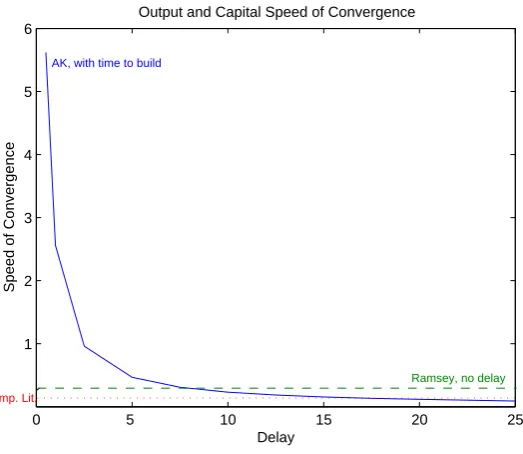
[image:23.595.173.435.128.355.2]Ramsey, no delay AK, with time to build
Figure 1: Speed of Convergence for different choices ofd.
of the stationary solutions. Of course, the main role is played by the delay pa-rameter which avoids the immediate adjustment of all the aggregate variables to their balanced growth path switching their speed of convergence from infi-nite to a fiinfi-nite value. In particular, the speed of convergence is measured by
ˆ
λ = |Re(λmax)−g|, with λmax the complex (and non real) root of the char-acteristic equation (8) having the highest real part; changes in the speed of convergence due to different choices of the time to build parameter are reported in Figure 1 after having calibrated the economy yearly.16
In the same graph, we have also reported a green line showing the speed of convergence to the steady state of a neoclassical growth model with Cobb Douglas technology and no time to build.17
. For a yearly calibration, the Ramsey model’s rate of convergence is around 7 per cent. On the other hand, the red line, at around 2 per cent, points out the empirical estimated value of the speed of convergence as documented in the literature (for a survey on econometric contributions refer to [17]).
This analysis indicates how time to build has to be considered a new different channel through which reducing the speed of convergence of growth models. On
16
More precisely we have setδ = 0.1, and σ = 1.5; the level of technology Aand the intertemporal preference rateρare let to vary in order to pin down the real interest rate
r= ˜Ae−ρdto five per cent a year.
17
the other hand the main aggregate variables in the AK model, converge too fast unless empirical implausible choices of the time to build parameter. Finally, it is also worth noting that introducing the time to build assumption triggers also in an AK model, the usual relations between the level of technology, the rate of intertemporal preference and the depreciation rate on the speed of convergence as pointed out in Proposition 2.2.
6
Conclusion
In this paper, we have shown how the close form policy function of an AK model with time to build can be found by using a not-standard Dynamic Programming approach, and how this result let us to fully explain the consumption smoothing effects induced by gestation lags in production. The differences and similari-ties with a vintage capital model having linear technology are also exploited by comparing the closed loop policy function in the two different frameworks and enlightening the different role of the equivalent capital. Finally several consid-erations on how delay in production may affect the global speed of convergence are proposed.
Appendix: Proofs
Proof of Proposition 2.1. First of all we prove (a). Let us define the function {
f(·) :R→R
f(·) :z7→z−Ae˜ −zd.
It can be easily seen that
lim
z→−∞f(z) =−∞ and zlim→∞f(z) =∞. (52)
Moreover the derivative off(·)is
f′(z) = 1 + ˜Ade−zd>0
sof is strictly increasing and by (52) it has a unique zeroξand this prove the first statement. Sincef(0) =−A <˜ 0 we have thatξ >0. Moreover
0<A˜(1−eAd˜ ) =f( ˜A)
so, sincef(·) is strictly growing, ξ < A˜. This prove the second inequality of the (9). The first can be proved observing first thatf(·)is concave, indeed it second derivative is given by
f′′(z) =−Ad˜ 2edz<0.
So, in particular, for all realz6= ˜A we have
f(z)< f( ˜A) +f′( ˜A)(z−A˜) = ˜A(1−e−Ad˜ ) + (z−A˜)(1 + ˜Ade−Ad˜ ), (53) and if we consider the unique zero
ξ0= ˜A
e−Ad˜ ( ˜Ad+ 1) 1 + ˜Ade−Ad˜ 6= ˜A
of the right hand side of (53) (it is just a straight line varyingz in R) we have
f(ξ0)<0 and sincef is growing andξis its unique zero the first inequality of (9) follows.
To prove the other parts observe first thatz is a root of (8) if and only if
w=zdis a root of
w= ˜Ade−w. (54) Now it is enough to apply Theorem 3.1 p. 312 of [10] to get (b), (c), (d).
The first statement of (e) follows from Theorem 3.12 p.315 of [10]. Indeed there it is stated that the sequence µk is strictly decreasing. The fact that
µk→ −∞ask→+∞follows since, rewriting (8) we have
dµk= ˜Ade−dµkcos(dνk), dνk=−Ade˜ −dµksin(dνk),
So from the second equation and the fact (coming from (d)) thatνk →+∞as
k→+∞, the claim follows.
Proof of Proposition 2.2. It is a simple application of the implicit function the-orem. For the rootξ one considers the function F( ˜A, d, ξ) = ξ−Ae˜ −ξd and
observe that
∂ξ ∂A˜ =−
∂F ∂A˜ ∂F ∂ξ
∂ξ ∂d=−
∂F ∂d ∂F ∂ξ
,
and make the straightforward computations.
For the rootµ1+iν1to simplify computations we use the fact thatz=µ+iν is a root of (8) if and only ifw=zd=: ¯µ+iν¯ is a root of
w=βe−w⇐⇒ {
¯
µ=βe−µ¯cos ¯ν
¯
ν =−βe−µ¯sin ¯ν . (55) whereβ = ˜Ad. Then we use the implicit function theorem to find ddβµ¯, dβdν¯ and then we use the fact thatµ¯=dµ,ν¯=dν and that β= ˜Adso
∂µ ∂A˜ =
1
d· ∂µ¯
∂β · ∂β ∂A˜ =
∂µ¯
∂β
∂µ ∂d =−
1
d2µ¯+
1
d ∂µ¯
∂β · ∂β ∂d =−
µ d2 +
˜
A d ·
∂µ¯
∂β
and then the claim follows by straightforward computations.
Proof of Proposition 2.3. The first part follows easily from the definition of
kM(·) and the positivity ofc(·). As proved in [3] ξ is the solution of (8) with highest real part, so the claim follows from [10] page 34.
Proof of Proposition 2.4. Forσ >1it is obvious sinceJ(k0(·);c(·))<0always. Forσ∈(0,1)we observe that for everyc(·)∈L1
loc([0,+∞);R+),
J(k0(·);c(·))≤
1 1−σ
∫ +∞
0
e−ρt(Akk0,c(t))
1−σd
t≤
≤ 1
1−σ
∫ +∞
0
e−ρt(AkM(t))1−σdt <+∞. (56)
where the last inequality follows from part (2) of Proposition 2.3.
Proof of Proposition 3.6. v is of course continuous and differentiable in every point ofX and its differential inxis
Dv(x) = (ν(1−σ)Γ(x)−σ,(1−σ)νΓ(x)−σψ1}) =νΓ(x)−σψ
SoDv(x)∈D(G)everywhere inX.
We can also calculate explicitlyGDvandAδ˜ −dDv, we have (using thatξsatisfies
the characteristic equation (8) and thenAδ˜ −d(ψ1) =ξ):
GDv(x) = (0,(1−σ)νΓ−σξψ1}) (57)
˜
Aδ−dDv(x) = (1−σ)νΓ−σξ >0 (58)
so
( ˜Aδ−dDv(x))−1/σ=αΓ(x) (59)
For the definition ofX ( ˜Aδ−dDv)−1/σ>0.
Ifx= (x0, x1)∈Y then
Γ(x)≤ 1
α A
˜
Ax
0 (60)
and then( ˜Aδ−dDv)−1/σ≤ AA˜x
0. So we can use Remark 3.4 and use the
Hamil-tonian in the form of equation (24).
Now it is sufficient substitute (57) and (58) in (24) and verify, by easy calcula-tions, the relation:
ρv(x0, x1)− h(x0, x1), GDv(x0, x1)iM2−
−x0Aδ˜ −dDv((x0, x1)−
σ
1−σ( ˜Aδ−dDv((x
0, x1))σ−1
σ = 0
Proof of Proposition 3.11. Clearlyφ∈C(M2). Givenp∈M2we have to prove
that {
d
dtxφ(t) =G
∗
xφ(t) + (0,Aδ˜ −d)(φ(xφ(t))), t >0
xφ(0) =p (61)
has a unique solution in Π. Unfortunately this cannot be done using known theorems available in the literature so we do it directly.
Informal description of the approach
We begin with an informal description of our approach: along the trajectories driven by the (candidate) feedbackφwe have (using the DDE notation, withu
andy):
u(t) =y(t)−α
(
y(t) +
∫ 0
−d
eξsAu˜ (t−d−s) ds+
)
=
y(t)α−αeξt
∫ t+d
t
If we take the derivative of such an expression and imposey˙(t) = ˜Au(t−d)we find
˙
u(t) = ˜Au(t−d)(1−α)−
−α(ξAe˜ ξt∫tt+de−ξsu(s−d) ds+ ˜A(−u(t−d) +e−dξu(t))). (63)
andu(0) =y(0)(1−α)−α∫−0deξsu(−d−s = ds. In the (rigorous) proof we
will consider (63), together with the equationsy˙(t) = ˜Au(t−d)and the initial conditions, as a starting point. We will prove the existence and uniqueness of the solution of such a DDE and, eventually, tranforming such DDE in the infinite dimensional setting, the existence and the uniqueness of the solution for (61).
End of the informal description of the approach
We consider the following DDE inu˜andy˜: ˙˜
u(t) = ˜Au˜(t−d) (1−α)− −α(ξAe˜ ξt∫t+d
t e
−ξsu˜(−d+s) ds+ ˜A(−u˜(t−d) +e−dξu˜(t))) t≥0 (64a)
˙˜
y(t) = ˜Au˜(t−d) t≥0 (64b) ˜
y(0) =y(0) (64c)
˜
u(s) =u(s) fors∈[−d,0) (64d) ˜
u(0) = (1−α)y(0)−α∫−0de
ξsAu˜ (−d−s) ds (64e)
that has an absolute continuous solution(˜u,y˜)on[0,+∞)(see for example [7] page 287 for a proof). Setting˜x:= (˜y,γ˜(t))where
˜
γ(t)[s] = ˜Au˜(t−d−s) fors∈[−d, s),
thanks to Theorem 3.2,x˜(·)satisfies, by (64b), (64c) and (64d),
{ d
dtx˜=G
∗˜
x(t) + (0,Aδ˜ −d)(˜u(t)), t >0
˜
x(0) = (y(0), γ(0))
Moreover, integrating (64a),
˜
u(t) = ˜u(0) +
∫ t
0
˜
Au˜(s−d) (1−α) ds−
−α
∫ t
0 [
ξAe˜ ξs
∫ s+d
s
e−ξru˜(−d+r) dr+ ˜A(−u˜(s−d) +e−dξ˜u(s))
]
ds=
(64)
(integrating by part in the double-integral term)
= ˜u(0) +
∫ t
0
˜
Au˜(s−d) (1−α) ds−
−α
(∫ 0
−d
eξru˜(t−d−r) dr
)
+αA˜
∫ d
0
(using (64e))
= (1−α) ˜y(0) +
∫ t
0
˙˜
y(s) (1−α) ds−α
(∫ 0
−d
eξru˜(t−d−r) dr
)
=
= ˜y(t) (1−α)−α
(∫ 0
−d
eξru˜(t−d−r) dr
)
=
= ˜x0(t) (1−α)−α
(∫ 0
−d
eξrx˜1(t)[r] dr
)
=φ(˜x(t)) (66)
and so {
d
dtx˜(t) =G
∗
˜
x(t) + (0,Aδ˜ −d)(φ(˜x(t))), t >0
˜
x(0) = (y(0), γ(0))
and thenx˜(t)is a solution of (61). The uniqueness follows from the linearity of
φso. This prove thatφ∈F Sp.
Proof of Theorem 3.12. To prove the first statement we take the derivative of the expressionΓ(xphi(t)) =hψ, xφ(t)i. Note that, sinceφis a feedback strategy
(Proposition 3.11) and φ ∈ D(G) (as observed in (27)) such derivative exists and (from (19)) we have
d
dtΓ(xφ(t)) =
d
dthψ, xφ(t)i=hGψ, xφ(t)i+ ˜Aδ−dψφ(xφ(t)) =
(thanks to the definition ofψgiven in (26)
=ξψ1, xφ(t)
+ ˜Ae−ξd((x0φ(t)−αΓ(xφ(t)))
)
= (sinceξ= ˜Ae−ξd)
=[ξψ1, xφ(t)+ξ(x0φ(t)
]
−ξαΓ(xφ(t))) =ξ(1−α)Γ(xφ(t))). (67)
This conclude the proof of the first statement.
To prove the invariance ofIc let us take ac <c¯and a p= (p0, p1)∈Ic. For
t≥0we have that (we callxφ simplyx)
u(t) =φ(x(t)) :=x0(t)−α
( ∫ 0
−d
eξsx1(t)[s] ds+x(t)0
)
(68)
where(x0(t), x1(t))is the trajectory starting fromp. Since, thanks to Theorem 3.11,φ ∈ F Sp then the trajectory (x0(·), x1(·)) is continuous and then u(·) is
continuous on[0,+∞). Let¯t∈[0,+∞)be, by contradiction, the first time such thatu(¯t)≤0oru(¯t)≥x0(¯t). We have
u(¯t) =x0(¯t)−α
( ∫ 0
−d
eξsx1(¯t)[s] ds+x(¯t)0
)
Since p1 ≥0 and u(t)> 0 for all t ∈ [0,¯t)then x0(t) is always growing18
on
[0,¯t]. Now fort≥0 ands∈[−d,0]we have:
x1(t)[s] =
{
p1[s−t] ifs−t >−d
˜
Au(t−d−s) ifs−t <−d (70)
Then, sincep∈I, we have, for almost everys∈(−d,0),
0≤x1(¯t)[s]≤cx0(¯t)
and so∫−0deξsx1(¯t)[s] ds≤ c ξ
(
1−e−ξd)x(¯t)0, then
0 < α
( ∫ 0
−d
eξsx1(¯t)[s] ds + x(¯t)0
) ≤ α ( c ξ (
1−e−ξd)+ 1
)
x(¯t)0 (71)
where the first inequality follows from the fact that x0(¯t) ≥ x0(0) > 0. So, from the first inequality of the (71) and from (69), we have immediately that
u(¯t)< x0(¯t). Moreover from (69) and the second inequality of (71) we have
u(¯t)≥x0(¯t)
[
1−α
(
c ξ
(
1−e−ξd)+ 1
)]
and then, thanks to the fact thatc <¯cwe have
0< u(¯t).
Summarizing u(¯t) > 0 and u(¯t) < x0(¯t) and this is a contradiction with the definition of ¯t. So, for t ≥0, u(t)∈(0, x0(t)). This also implies that x0(t)is always growing and then (sincex0(0)>0) anways strictly positive. Thanks to the relation (70)Ic is an invariant set and we have the claim.
Proof of Corollary 3.13. It follows easily by the fact that by Theorem 3.12, ev-eryIc is invariant.
Proof of Theorem 3.15. 1. To prove that I ⊆ Y we have only to verify that for everyIc (with c < c¯) Ic ⊆X and the inequality appearing in the (29) is
satisfied. The first fact follows by the strict positivity ofx0and by the positivity ofx1(·)of the element ofI
c. To prove the inequality appearing in (29) we have
only to observe that, onI
(∫ 0
−d
eξsx1[s] ds+x0
) ≤ ( c ξ (
1−e−ξd)+ 1
)
x0< 1 αx
0≤A
˜ A 1 αx 0 18
Sincex0(t)solves the DDE:
x0(t) =p0(0) +
Zt∧d
0
p1[−s] ˜ A ds+
Z (t−d)∧d
0
u(s) ds.
where the first inequality follows from the definition ofIc (as in (71)) and the
second by Hypothesis 3.14 and by the definition of¯c. So we have that I ⊆Y. We take nowp ∈I, in particularp∈ Ic for some Ic with c <¯c. Considering
the evolution of the system starting frompand driven by the feedbackφis the same that considering the evolution of equation (35) starting fromp. But from Theorem 3.12 we know that Ic is invariant for the flow of (35) and then the
trajectory starting fromp∈Icremains inIc and then, sinceIc⊆Y, remains in
Y and then, thanks to the definition ofY and the fact that along the paths of (35) we have (68) we have thatu(·)∈ A0(p)and so φ∈AF Sp.
2. Now we prove that φ∈OF Sp. We considerv as defined in Proposition
3.6. From what we have just said on the admissibility ofu(t)follows thatx(·)
remains inY as defined in (29) and so the Hamiltonian can be expressed in the simplified form (24) recalled in Remark 3.4. Moreover, thanks to Theorem 3.6
vis a solution of HJB on the points of the trajectory. We introduce:
{
˜
v(t, x) :R×X→R ˜
v(t, x) :=e−ρtv(x) (v is defined in(30)). (72)
Using that(Dv(x(t)))∈D(G)and that the functionx7→Dv(x)is continuous with respect the norm ofD(G)(see the proof of Proposition 3.6 for the explicit form ofDv(x)), we find:
d
dtv˜(t, x) =−ρ˜v(t, x(t)) +hDx˜v(t, x(t)), G
∗
x(t) + ( ˜Aδ−d)
∗
u(t)iD(G)×D(G)′
−ρe−ρtv(x(t)) +e−ρt(hGDv(x(t)), x(t)iM2+ ( ˜Aδ−d)Dv(x(t))u(t)
) (73)
By definition (recalling thatu(·) =φ(x)(·)):
v(p)−J0(p, u(·)) =v(x(0))−
∫ ∞
0
e−ρt(x
0(t)−φ(x)(t))1−σ
(1−σ) dt=
Then, using (73) (using Proposition 2.3 to guarantee that the integral is finite and that the “boundary term at∞” vanishes), we obtain
=
∫ ∞
0
e−ρt
(
ρv(x(t))− hGDv(x(t)), x(t)iM2− h( ˜Aδ−d)Dv(x(t)), u(t)iR )
dt−
−
∫ ∞
0
e−ρt
((
x0(t)−u(t))1−σ
(1−σ)
)
dt=
=
∫ ∞
0
e−ρt
(
ρv(x(t))− hGDv(x(t)), x(t)iM2
−h( ˜Aδ−d)Dv(x(t)), u(t)iR−
(x0(t)−u(t))1−σ
(1−σ)
)
using Theorem 3.6
=
∫ ∞
0
e−ρt
(
H(x(t), Dv(x(t)))− HCV(x(t), Dv(x(t)), u(t))
)
dt (74)
The conclusion follows by three observations:
1. Noting that H(x(t), Dv(x(t))) ≥ HCV(x(t), Dv(x(t)), u(t)) the (74)
im-plies that, for every admissible control λ(·), v(p)−J0(p, λ(·)) ≥ 0 and thenv(p)≥V0(p).
2. The original maximization problem is equivalent to the problem of find a controlλ(·)that minimizev(p)−J0(p, λ(·))
3. The feedback strategyφachievesv(p)−J0(p, u(·)) = 0that is the minimum in view of point 1. Moreover this implies thatv(p)≥V0(p).
Proof of Proposition 4.4. The first statement follows by Theorem 3.12. In view of Proposition 4.2 along optimal trajectory we have:
Λegt=y∗(t)−u∗(t) =α
( ∫ 0
−d
˜
Aeξsu∗(t−s−d) ds+y∗(t)
)
so to compute the explicit value ofΛ we only have to compute the value of the right side at time0and we find
Λ =α
( ∫ 0
−d
eξsAu˜ (−s−d) ds+y(0)
)
.
This concludes the proof.
Proof of Proposition 4.6. The existence of the limityL fory¯(t) is proved in [3]
(in Proposition 2 page 1027 the author proves the existence of the limit for
¯
k(t) = A1y(t+d)). This implies, thanks to Corollary 4.5 the existence of the limit uL. We can here compute explicitly the value of such limits using the
explicit form of the optimal feedback (37). Namely we have only to impose, from (37)
uL=yL−α
(
yL+ ˜A
∫ 0
−d
eξsuLe−gse−gdds
)
=
=yl(1−α)−
1−e−(ξ−g)d
ξ−g uLαAe˜
−gd (75)
and then
uL=yL
1−α
1 + 1−e−(ξ−g)d
ξ−g αAe˜
Moreover from Corollary 4.5 we have that
uL=yL−Λ. (77)
Using (76) and (77) we find:
yL= Λ
(
1− 1−α 1 +1−e−(ξ−g)d
ξ−g αAe˜
−gd
)−1
and
uL= Λ
(
1− 1−α 1 +1−e−(ξ−g)d
ξ−g αAe˜
−gd
)−1 −1
and so we have the claim.
Proof of Theorem 4.7. All the statements are corollaries of the results of Section 4. More precisely:
1. Follows from Lemma 4.4 and by relations (42)-(43).
2. Follows from the previous point and (1).
3. Follows from Proposition 4.1 and by relations (42)-(43).
4. Follows from Proposition 4.6 and by relations (42)-(43) and by (16).
5. Follows from the point 4 above and [6].
References
[1] Asea, P.K. and Zak, P.J. (1999), “Time-to-build and cycles”, Journal of Economic Dynamics and Control, vol.23, no.8, 1155-1175.
[2] Barro, R. J., Sala-i-Martin, X., 2004. Economic Growth. Second Edition. The MIT Press.
[3] Bambi, M. (2008), “Endogenous growth and time to build: the AK case”, Journal of Economic Dynamics and Control, vol. 32, 1015-1040.
[4] Bambi, M., and Gori, F. (2009), “Unifying time to build theory”.
[5] Benhabib, J., and Rustichini, A. (1991), “Vintage capital, investment, and growth”, Journal of Economic Theory 55, 323-339.