Automatic Plant Branch Segmentation and Classification Using Vesselness Measure
Z. Mohammed Amean
[email protected] 1, 2 & 3 T. Low
[email protected]. 1&2 C. McCarthy
[email protected]. 2 N. Hancock
[email protected]. 1&2
1 Faculty of Engineering and Surveying, University of Southern Queensland, Toowoomba, QLD 2 National Centre for Engineering in Agriculture, West Street, Toowoomba, QLD
3 Control and Systems Engineering, University of Technology, Baghdad, Iraq
Abstract
Remote monitoring of plant vegetation is an effective method to save time and to improve production efficiency. Modern agriculture techniques utilise mobile robot and machine vision for automated image acquisition and analysis. The Identification of plant parts such as leaves, stem, branches and flowers is important for assessing plant growth, irrigation strategy and plant health. In this paper, automatic segmentation and counting of plant branches based on vesselness measure and Hough Transform techniques is presented. Frangi 2D filter, based on Hessian matrix eigenvalues has been used to classify image pixels as either tube-like or blob-like. First the input image was converted to the gray scale image and used as input to the Frangi 2D filter. Size filter was used to eliminate non-branches and small objects from the image. Hough Transform was applied to detect and draw lines on the stem and branches on the image. The developed method can detect and count the branches automatically and was applied on different sides of view and different illumination conditions for the same plant. The results show a high percentage of branches segmentation for clear side views of the plant. However, branch segmentation was affected by low illumination conditions.
1 Introduction
Efficient segmentation of plant features is one of the major requirements for precision agriculture. Plants and trees are the most complex of nature’s objects thus, multiple image analysis techniques should be used to segment plant features. Plant identification based on analysing plant images features has provided benefits for agronomy and biology for plants species identification.
Stem detection of plants is also useful for plant modelling. Plant modelling can be used to monitor plants for many purposes such as the growth stage, plant health, and yield estimation and to improve input resources management. Machine vision can be used to discriminate useful data from plant images. Feature extraction, image segmentation and feature matching are the main steps of image processing techniques that researchers currently use to detect plant parts. Image segmentation makes an image more meaningful and easier to analyse and extract useful data. Plant parts are usually classified according to their colour, shape and structure of their stem, leaves and flowers [Valliammal and Geethalakshmi, 2011].
1.1
Related Work
then updating the plant skeleton structures and estimates the plant centre position. This system has a promising performance in detecting individual and overlapped corn plant with 96.7% correctly detected under natural lighting conditions. Previous work in cotton with line detection of stem and internodes length was implemented by McCarthy et al., [2009]. A single camera is used to measure the distance between nodes on the main stem, which is a significant indicator of plant water stress and irrigation crop management. The image analysis consisted of a first stage to identify candidate nodes from individual images and then a second stage where false positive nodes were removed by comparing a sequence of images. The system used a monocular video acquisition system that required contact with the plant to obtain dimensional measurement. An attempt to model a maize canopy in three dimensions was presented by Ivanov et al., [1995] based on stereovision. The images were taken from a top height of 8.5 meters above the ground and the canopy geometrical structure was analysed to estimate the leaf position and orientation.
Other researchers used phenotyping analysis technique to measure and segment the features of plants. Kaminuma et al., [2004] presented a method of phenotypic analysis based on precise three-dimensional 3D measurement using a laser range finder (LRF). The method was capable of measuring the geometry of young plants and provides precise descriptions compared to conventional 2D measurement, while Chéné et al., [2012] used a low cost depth camera for entire plant phenotyping with 3D measurement using a single top view. For more complex overlapping plants Noordam et al., [2005] compared techniques of stereo imaging, laser triangulation, X-ray imaging and reverse volumetric intersection (RVI), to locate the stem position for a rose cutting robot. The result shows the RVI is most promising to locate the stem down to the cutting position in terms of robustness and costs. Waksman et al., [1997] used stem flaccidity and leaf pallor as a good indication of the thirstiness of a plant.
In this paper, an algorithm has been developed using novel combination techniques to extract stem plant features from the colour side view of the image in an indoor environment. The algorithm consists of three steps: 1- extract branches from colour plant images using vesselness measure and, 2- apply the Hough Transform to detect lines of the branches and 3- classify those branches according to the Hough transform parameters and count those branches automatically and present them in different colours.
2
Collected Images Experiment
Images were captured using 8-bit RGB colour stereo vision camera. The Bumblebee2 stereo vision camera can capture mono and stereo vision images in indoor and outdoor conditions. The resolution of images used is 384 x 512 pixels. The images taken were of a hibiscus nursery plant from different aspects at different indoor illumination conditions (Figure 1). The images were taken from a constant distance of 100 cm. Stereo vision cameras have the ability to produce disparity images and point cloud data that gives the depth information about the plant parts and the distance between the plant and camera. Depth information will be useful to model the stem and branches in 3D dimensions. Matlab 2012b and TriclopsDemo software were used for software development.
3 The Vesselness Measure
1996]. Waksman et al., [1997] used line detection technique to detect leaf stems in vine images and the identification of blood vessels in medical images [Frangi
et al., 1998].
In our case a Frangi 2D filter has been used to extract vessel structures of branches and stem. A Frangi 2D filter was used by Qian et al., [2008] to detect vessels for complex vascular structure, Tankyevych et al. [2008] for filtering thin extended objects (such as veins and fibres) and Tankyevych et al. [2009] for blood vessel edge enhancement and reconnection, McCarthy et al., [2009] for automated detection of internodes of cotton plant stem, and [Schneider and Sundar, 2010] for automatic vessel segmentation. In contrast to the plant biology and agriculture literature, the medical literature is more extensive with respect to curvilinear line detection [McCarthy et al., 2009]. This technique calculates the eigenvalues and eigenvectors of the Hessian matrix (H) to compute the likeness of an image region to vessels, according to method described by Frangi et al., [1998]:
xx xy xy yy
I
I
H
I
I
………... (1)
Where
2
ab
a b
I
I
for each image pixel, and I is thepixel’s intensity value [Magnus and Neudecker, 1999]. The image second order derivatives are calculated by convolving the image with derivatives of a Gaussian kernel with standard deviation ơ [Steger, 1996]. Vessel structures and lines with different widths can be extracted by varying the standard deviation of the smoothing filter ơ. Wider lines can be detected with a large value of ơ. In our algorithm different values of ơ were investigated to select the suitable value for branch detection and segmentation.
The eigenvalues of Hessian matrix (H) are symbolized as
1
and
2 can be used to detect the vessel region [Frangi et al., 1998].The eigenvalues decide if this pixel belongs to a ‘tube-like’ or a ‘blob-like’. A small value of
1 witha large value of
2 indicates that this pixel belongs to a ‘tube-like’ structure. The sign of eigenvalues indicates the brightness of the tube structure. The vesselness is a measure of the probability of the pixel belonging to a blood vessel [Frangi et al., 1998]. In our case the vesselness is a measure of the probability of the pixel belonging to the plant stem and branches.The vesselness measure consists of two criteria, the ‘second order structure’
s
which gives a low response forlow image contrast and the ‘blobness measure’ [Frangi et al., 1998]. The ‘second order structure’
s
is calculated by using the expression:s
1 2
2 2for2D image.
The blobness is given by the ratio of the Hessian
matrix eigenvalues
1/
2 and it has low value for ‘tube-like’ than ‘blob-‘tube-like’ structures. The vesselness measure
v
can combined between ands
by the expression of Equation 2 where andc
are thresholds which control the filter’s sensitivity to ands
, respectively.2
2
2 2
2
exp 1 exp 0;
2 2
0 otherwise.
s if
v c
.….. (2)
3.1 Size Filter and Hough Transform
A Morphological size filter has been used to minimize the small connected component on binary images. To fit a line to the vesselness measure, Hough Transform [Duda and Hart, 1972] has been used to identify the main stem and branches of the plant. Hough Transform uses a voting technique to identify points located on the same line and has a good performance to detect the stem and branches properly.
4 Plant Segmentation Algorithm
The developed algorithm consists of the following steps:
1. Apply Frangi 2D filter on the gray scale image to segment branches and the stem.
2. Use morphological size filter to remove other non-branch objects.
3. Apply Hough Transform (lines) to find the segmented branches.
4. Use Hough Transform parameters (
,
) to classify detected lines and store the lines which share the same parameters (or close values) in the same bin.5. Count the number of branches by counting the numbers of bins.
6. Hough transform draws multiple lines for each segmented branch, our algorithm uses other parameters of the Hough Transform (the value of x and y coordinate for each line points) to arrange those points in ascending order and draws a single line for each branch.
7. Validate the points of each line and delete any points greater than a threshold distance away.
8. Classify each branch and present it in a different colour.
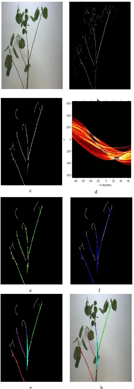
[image:3.612.57.286.339.425.2]5 Results and Discussion
5.1
Vesselness Measure for Branch Detection
In order to evaluate the performance of our algorithm we selected 12 images. The images of a Hibiscus nursery
plant were captured at different indoor illumination conditions from different sides of view. First the
algorithm read the colour image and converted it to gray-
scale to apply the 2D Frangi filter. Under good light conditions, good results can be obtained by choosing low value of standard deviation ơ for the smoothing filter. On the other hand, other images with poor illumination need a high standard deviation value ơ. The stem and branches areas yield high Hessian eigenvalues compared to the leaf
[image:4.612.54.288.49.726.2]areas, thus leaf areas can be eliminated using size filter.
Figure 3 shows a Hibiscus nursery plant from an arbitrary side of view under indoor conditions with the output of
2D Frangi filter.
The plant images show different responses of the
vesselness measure to the stem and branches with varying values of standard deviation ơ. By increasing the value of ơ, the width of the detection line increases as well as the detection of blob leaf areas can be recognised and
increase which as the blobness increased. The
brightness of detected branches can be controlled by
setting a suitable value to and
c
(the parameters of Equation 2). In this study we are concerned with the detection of stem and branches, thus a low value of standard deviation ơ was chosen to detect stem and branches correctly and to eliminate the leaf areas. The parameters selected by empirical testing (ơ = 0.55, = 0.5 andc
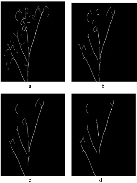
= 7) to segment branches only and not the edge of leaves.5.2 Edge Detection Filter for Branch Detection
Edge detection was also used as a filter to detect stem and
branch edges. From the literature, Sobel [Sobel & Feldman, 1968] and Canny [Canny, 1986] edge detection
has been demonstrated to be more effective and a more
accurate method for edge detection of plant parts (i.e. leaves as well as stems). Figure 4 shows plant output a
Figure 2. The output process of the developed algorithm. (a) RGB image, (b) Frangi filter output, (c) size filter, (d) Hough Transform accumulator, (e) Hough Transform Output multiple lines for each branch, (f) Reduces lines to a single line for each branch, (g) counts those lines and assigns different colour for each lines and (h) overlapped those lines with the original image.
b
a b
d
e f
g h
segmentation after applying Sobel and Canny edge detection. It is clear that the Sobel filter detects stem,
branches and leaves boundary area while Canny filter detects stem, branches, leaves boundary area and leaf
veins. The Sobel filter threshold was adjusted to a value
of (0.0712) while it takes values ranging from (0.0125-0.0313) for Canny filter with sigma value equal to one.
The parameters values were observed to achieve the clearest stem and branches but it also extracted leaves as
well. Our algorithm concerned with stem and branch detection, therefore the Frangi filter is more effective for
our application.
Figure 5 Demonstrates the output after applying a morphological size filter with a different value of connected component for selected value of standard
deviation (ơ = 0.55) as shown in Figure 3 (b). Size filter
works under the concept of connected component, which mean the filter removes all connected components (objects) that have less than selected ‘x’ pixels. ‘x’ can
take any integer positive value. The optimal value of size filter can be obtained when ‘x’ value equals 50 in order to eliminate the leaf areas and to keep stem and branches
area without missing information as shown in Figure 5 c.
Figure 3. Hibiscus nursery plant (a) RGB image, (b), (c) and (d) the output of Frangi 2D filter with standard deviation ơ = 0.55, 2.55 and 4.55 respectively.
Figure 5. Different values of size filter for the image of Figure 2 (b), a=10, b=30, c=50 and d=70 respectively.
b a
c d
Sobel both threshould edge detection Canny edge detection
Figure 4. Hibiscus nursery plant (a) Sobel edge detection filter and (b) Canny Edge detection filter.
[image:5.612.324.559.119.293.2] [image:5.612.56.288.231.575.2] [image:5.612.326.560.349.661.2]5.3 Hough Transform Parameters
Hough Transform has been applied to detection lines of
the stem and branches. Since illumination conditions affected the brightness of stem and branches, Hough
Transform did not work well under poor illumination
conditions. Figure 6 shows the output of the Hough Transform accumulator. The small black square points
represent the values for each stem detected by the Hough Transform technique. There are five groups of those small
square points which represent the detection of five branches. Each group has similar parameter values
(
,
) or very close together as shown in figure 6. TheHough transform Technique put all this groups in one bin as mentioned in the plant segmentation algorithm (section
4).
Our algorithm works on those parameters by classifying
them as a group and putting each group in one bin. The number of bins represents the number of branches. The
Hough Transform represents each branch by multiple
lines as shown in figure 2 (e), the developed algorithm minimises those lines to a single line for each branch as
shown in Figure 2 (e). Finally the developed algorithm differentiates between the lines by rendering them in
different (false) colours as shown in Figure 2 (g) and (h).
5.4
Discussion of Branch Detection Results
The algorithm was applied to 12 images of a Hibiscus
nursery plant from different aspects of the plant facing the camera. Figure 7 column A shows samples of these
images at indoor condition from different perspectives and different illumination conditions. Figure 7 column B
shows varying percentage of response of the developed
algorithm to those images. The first row images represent the plant from a clear position facing the camera and
indoor illumination condition (artificial light) and typical response from the developed algorithm. All five branches
are correctly detected by the Frangi filter and Hough
Transform technique.
[image:6.612.332.588.213.702.2]A B
Figure 7. Hibiscus nursery plant, (A) RGB image, (B) response of the developed algorithm.
1
2
3 4
5
Non detected branch
Non detected branch
(degrees)
-80 -60 -40 -20 0 20 40 60 80 -600
-400
-200
0
200
400
600
[image:6.612.51.295.291.486.2]0 0.1 0.2 0.3 0.4 0.5 0.6 0.7 0.8 0.9 1
Figure 6. Hough Transform Accumulator output for the image of figure 7 Row 1. The groups are numbered as branches number in the image of Figure 7.
Group of branch 4
Group of branch 5
Group of branch 2
Group of branch 1
The algorithm counts them as five branches and presents them in five different colours. Figure 7, row 2 shows the
same plant from another aspect under indoor conditions with sun light illumination only (without artificial light).
One of the right side branches is not detected by the
vesselness measure properly because of the shadow of the other branch. As such it is not counted by the algorithm.
The actual number of branches that can be counted from this side of the image is eight and the algorithm detects
only seven branches. Figure 7, Row 3 shows good indoor illumination conditions (artificial light). The algorithm
detects and counts three branches from four, because the
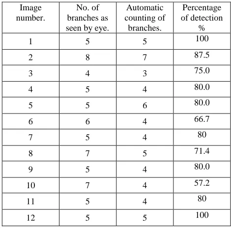
fourth branch on the left side of plant was shaded by the branch leaves. Table 1 shows the response of these
images to our algorithm. The first three rows of the table show the result of Figure 7.
The other images are the same plant images that were used to evaluate the algorithm under different conditions.
Images 1, 3, 8, 9, 10, 12 were in artificial light and the others were in sunlight. The number of plant branches is
five as counted from the ground truth. The second column
represents the number of branches as can be seen by eye from different side views of images, while the third
column shows the automatic counting of branches by the developed algorithm. It is clear there is a difference
between the actual number of branches and the automatic
counting number. The algorithm deals with the images thus, the number of branches depends on how many
branches can be seen from specific side of images and the illumination intensity applied as mentioned before. Image
1 of Table 1 (Figure 7, Row 1) shows that the number of branches is five and they were counted as five by the
algorithm.
Row 1 and row 12 of Table 1 represent the typical response of the developed algorithm because 100% of branches have been detected correctly. This optimal
response to our algorithm is due to the good illumination
conditions and clear view of plant from the camera which are significant factors for proper detection and counting.
The other images of Table 1 show a different response of the developed algorithm to detecting and counting plant
branches with a high percentage of accuracy. The number
of branches in the image is different from image to image depending on side view of the image. The illumination
condition also affected the performance of the algorithm. Good illumination conditions mean good vesselness
measure, good Hough transform detection, thus the developed algorithm can classify Hough Transform lines
in bins and count bins correctly.
5 Conclusion and Future Work
The automatic detection and counting of plant branches was demonstrated. The detection of branches was
achieved by applying the vesselness measure and Hough Transform technique. The vesselness measure was more
effective in detecting branches than edge detection filters
(Sobel, Canny) because, edge detection filters detect all the details of plant structure such as leaves and leaf veins.
A Hibiscus nursery plant was used to evaluate the new algorithm. The result showed that 2 of 12 images were
properly detected by the algorithm, 7 of 12 were detected with one missing or an extra number of branches, while
the rest were presented with two or three undetected
branches. Two parameters affected those results; good illumination conditions and clear view of plant from the
camera. The overall accuracy of the developed algorithm is good.
Further work on enhancing the algorithm can be expected by applying the algorithm to more images of different
plants to obtain more statistical data and apply the algorithm on more complex structure plants. Using a
Image number.
No. of branches as seen by eye.
Automatic counting of
branches.
Percentage of detection
%
1 5 5 100
2 8 7 87.5
3 4 3 75.0
4 5 4 80.0
5 5 6 80.0
6 6 4 66.7
7 5 4 80
8 7 5 71.4
9 5 4 80.0
10 7 4 57.2
11 5 4 80
[image:7.612.329.564.108.342.2]12 5 5 100
stereovision camera with depth information combined with the colour information can enhance branch detection.
Depth images can enhance branch detection by adding the
third dimension to the plant image.
6 Acknowledgements
The senior author would like to acknowledge the ministry
of Higher Education in Iraq who sponsored the PhD scholarship.
References
[Canny, 1986] J. F. Canny. A computational approach to edge detection. IEEE Trans Pattern Analysis and Machine
Intelligence 8: 679-698, 1986.
[Chéné et al., 2012] Yann Chéné, David Rousseau,
Philippe Lucidarme, Jessica Bertheloot and Valérie Caffier. On the depth camera for 3D phenotyping of entire
plants. Computer and Electronics in Agriculture,
82:122--127, March 2012.
[Chien and Lin, 2005] Chung F. Chien and Ta T. Lin.
Non-destructive growth measurement of selected vegetable seedlings using orthogonal images.
Transactions of the ASAE, 48:1953—1961, August 2005.
[Duda and Hart, 1972] Richard O. Duda and Peter E.
Hart. Use of the Hough Transformation to detect lines and curves in pictures. Communications of the ACM, 15:11—
15, January 1972.
[Frangi et al., 1998] Alejandro F. Frangi, Wiro J. Niessen, Koen L. Vincken and Max A. Viergever. Multiscale
vessel enhancement filtering. Lecture Notes in computer Science, 1496: 130—137, October 1998.
[Ivanov et al., 1995] N. Ivanov, P. Boissard, M. Chapron and B. Andrieu. Computer stereo plotting for 3-D
reconstruction of a maize canopy. Agricultural and forest
meteorology, 75: 85—102, June 1995.
[Jing and Tang, 2009] Jian Jin and Lie Tang. Corn plant
sensing using real-time stereo vision. Journal of Field Robotics, 26: 591—608, June - July 2009.
[Kaminuma et al., 2004] Eli Kaminuma, Naohiko Heida,
Yuko Tsumoto, Naoki Yamamoto, Nobuharu Goto and Naoki. Automatic quantification of morphological traits
via three-dimensional measurement of Arabidopsis. The
Plant Journal, 38: 358—365, January 2004.
[Magnus and Neudecker, 1999] Jan R. Magnus and Heinz
Neudecker. Matrix Differential Calculus with Applications in Statistics and Econometrics, Revised
Edition, John Wiley & Sons, 1999.
[McCarthy et al., 2009] Cheryl L. McCarthy, Nigel H.
Hancock and Steven R. Raine. Automated internode length measurement of cotton plants under field
condition. American society of agricultural and Biological
Engineers, 52: 2093—2103, November 2009.
[Noordam et al., 2005] J.C. Noordam, J. Hemming, C.
van Heerde, F. Golbach and R. van Soest. Automated Rose Cutting in Greenhouses with 3D Vision and
Robotics: Analysis of 3D Vision Techniques for Stem Detection. Proceeding of the International Conference on
Sustainable Greenhouse Systems, pages 885-892, Leuven,
Belgium, October 2005.
[Otsu, 1975] Nobuyuki Otsu. A threshold selection
method from Gray-Level Histograms. IEEE Transaction on Systems, Man and Cybernetics, 9: 62—66, January
1979.
[Qian et al., 2008] Xiaoning Qian, Matthew P. Brennan, Donald P. Dione, Wawrzyniec L. Dobrucki, Marcel P. Jtackowski, Christopher K. Breuer, Albert J. Sinusas and
Xenophon Papademetris. A non-parametric vessel
detection method for complex vascular structures. Medical Image Analysis, 13: 49–61, February 2009.
[Schneider and Sundar, 2010] Automatic global vessel segmentation and catheter removal using local geometry
information and vector field integration.
[Sobel and Feldman, 1968] I. Sobel and G. Feldman. A 3×3 isotropic gradient operator for image processing.
Presented at a talk at the Stanford Artificial Project.
[Steger, 1996] Carsten Steger. Extracting curvilinear
structures: a differential geometric approach. Lecture Notes in Computer Science, 1064: 630–641, 1996.
Biomedical Imaging: From Nano to Macro, pages 45 –
48, Rotterdam, Netherlands, April 2010.
[Tankyevych et al. 2008] Olena Tankyevych, Hugus
Talbot and petr Dokladal. Curvilinear Morpho-Hessian filter. Proceedings of the 5th IEEE International
Symposium on Biomedical Imaging: From Nano to Macro, pages 1011-1014, Paris, France, May 2008.
[Tankyevych et al. 2009] Olena Tankyevych, Hugus Talbot, petr Dokladal and Nicolas Passat.
Direction-adaptive grey-level morphology. Application to 3D vascular brain imaging. Proceedings of the 16th IEEE
International Conference on Image Processing, pages
2261 – 2264, Cairo, Egypt, November 2009.
[Valliammal and Geethalakshmi, 2011] N. Vallimmal and
S.N. Geethalakshmi. Automatic recognition system using preferential image segmentation for leaf and flower
images. Computer Science & Engineering: An
International Journal. 1: 13—25, October 2011.
[Waksman and Rosenfeld, 1997] Adlai Waksman and Azriel Rosenfeld. Assessing the condition of a plant.