Frequency tracking and hidden Markov models

70 %, is my own.

realization problem. We consider issues such as equivalence of nonnegative linear systems (HMMs), state aggregation, approximation of nonnegative linear systems (HMMs) by lower order nonnegative linear systems (HMMs) etc. We first present the results in the literature in a unified matrix algebra framework which makes it easier to address some computational issues. We then obtain some new results and additionally some existing results in the literature are either extended or simplified. We also give some analysis on how to use stochastic complementation techniques to approximate a HMM by another HMM with a lesser number of states.

References

[1] R. L. Streit and R. Barrett, “Frequency line tracking using hidden Markov models,”, IEEE Transactions ASSP, vol. 38, no. 4, pp. 586-589, 1990.

[2] R. L. Streit, “The moments of matched and mismatched hidden Markov models”, IEEE Transactions ASSP, vol. 38, no. 4, pp. 610-622, 1990.

[3] S. Kullback, Information Theory and Statistics, Dover Publications, Inc., New York, 1968.

3 Performance of HMM-ML Frequency Trackers 55

3.1 Introduction... 55

3.2 A formulation of hidden Markov m o d e ls ... 58

3.3 The HMM-ML frequency tr a c k e r ... 59

3.4 HMM Viterbi state sequence estimation algorithm... 64

3.5 A performance analysis of HMM-ML frequency tra c k e rs ... 66

3.5.1 Constant frequency c a s e ... 67

3.5.2 Simulation studies for constant frequency s ig n a ls ... 72

3.5.3 Random walk frequency c a s e ... 74

3.5.4 Simulation studies for random walk frequency signals... 77

3.5.5 Autoregressive frequency variations... 84

3.5.6 Simulation studies for AR frequency signals... 86

3.6 Conclusion... 87

References ... 92

4 Matched and Mismatched Moments of Hidden Markov Models 95 4.1 Introduction... 95

4.2 Moments of output sequence probabilities of HMMs ... 96

4.3 A simple calculation of the moments of output sequence probabilities of HMMs 100 4.4 E x am p le...101

4.5 Conclusion ... 102

4.A Appendix ... 103

References ... 105

5 A Calculation of a Distance Between Hidden Markov Models 107 5.1 Intro d u ctio n ...107

5.2 The calculation of the KL number between HMMs using Streifs conjecture . . 108

5.3 The analysis of Streit’s conjecture using Bernoulli c h a in s ... 112

5.4 Modification of Streit’s conjecture... 114

5.5 Examples ...116

5.6 Conclusion...117

References ...118

A Convex cones and their properties 253 References ... 256

3.8 RMSE of the frequency estimates for random walk frequency variations with respect to frequency jumping probability... 83 3.9 RMSE of frequency estimates obtained by a HMM-ML frequency tracker for

AR frequency signals when signal block length N was 6 4 ... 90 3.10 Comparison of the signal length for the performance of HMM-ML frequency

tracker for AR frequency v a ria tio n s ... 91

6.1 The trajectory of the states of a rank-minimal system with nonnegative inputs . . 146 6.2 The admissible regions of the eigenvalues of third and fourth order stochastic

m a tr ic e s ...147 6.3 The frequency responses of a nonnegatively-minimal linear system and its ap­

proximate system ... 160 6.4 The frequency responses of a nonnegatively-minimal linear system and its ap­

proximate system ... 161

7.1 A HMM with three states and two output sy m bols... 175 7.2 The infinite-dimensional matrix H^l\ P ) with its linearly independent columns . 229

2

methods can be found in [2].

Another important application of HMMs is in the area of frequency tracking where one would like to track the frequency of a noisy sinusoidal signal whose frequency varies slowly during the measurement interval. The hidden Markov model-maximum likelihood (HMM-ML) frequency tracker given in [3] and [4] is a good example how HMMs can be useful in frequency tracking. A block diagram of the HMM-ML frequency tracker in [3] is given in Figure 1.1. A more explicit discussion on the HMM-ML frequency tracker will be given later. However, we should note that although the HMM-ML frequency tracker given in [3] has proved itself to be useful in frequency tracking, its performance in noisy environments and for different frequency variations is not well investigated, apart from some simulation studies. In this thesis, we were motivated by this lack of a theoretical performance analysis of the HMM-ML frequency tracker in the literature. During our investigations, we also came across some open problems related to HMMs which are important both theoretically and practically. One of them is that there is no computationally efficient way of calculating a “distance” between discrete output symbol HMMs. Another fundamental problem is to find the parameters of a HMM from its output sequence probabilities. Solutions for these problems are necessary to have a solid understanding of HMMs so that their practical applications can be improved, including their use in the frequency tracking area, namely the HMM-ML frequency tracker. With the inclusion of a performance analysis of the HMM-ML frequency tracker, these three topics are the main themes of this thesis. In other words, the research carried out for this thesis can be grouped mainly under three topics which are

(i) A performance analysis of the HMM-ML frequency tracker,

(ii) An investigation of a calculation of a probabilistic distance between discrete output symbol HMMs,

(iii) HMM realization theory.

4 Chapter 1. Introduction

A noisy sinusoidal signal with a

time-varying "frequency"

Constant frequency estimates

for the signals in the blocks

Time Domain

Blocking

Rife & Boorstyn

constant frequency

estimator

HMM Viterbi

state sequence

estimator

Estimated frequency

track

6 _{Chapter 1. Introduction}

is given by

= f t » , « { * [1] = » } • (1.3) Note that the HMM parameters A, B and n are constant and furthermore if IT is the stationary distribution on the HMM states then the stochastic vector II also satisfies II A = II.

The probability of an output sequence realization over an interval of arbitrary length T, call it V\ = (*/[!], y[2], • • •, y[T])y is given by

P * N, M

{ yiT =

}

=

n

•

1

(1 -4)

where 1N is an N-dimensional column vector of ones and Bk for k = 1 , 2 , . . . , M are N x N-dimensional diagonal matrices whose j-th diagonal entries are given by bkj which is equal to P \ N M{y[t\ = k I X[t] = j } f o r j = 1 , . . N . Here Y f = ( y [ l ] , . . Y[T]) denotes a random output sequence of the HMM \n}m

-Having defined HMMs, let us now consider the first major topic in this thesis which is an application of HMMs in the frequency tracking area, viz. the HMM-ML frequency tracker. The following subsection gives some background material and motivation for this topic.

1.1.1 F re q u e n c y tra c k in g

In areas such as sonar and radar [6], one usually needs to estimate the parameters of a noisy sinusoidal signal, particularly its frequency. When the signal frequency is constant during the measurement interval, one can use a maximum-likelihood (ML) constant frequency estimator whose asymptotic properties are quite well known, as shown for example in [7]. On the other hand, when the signal frequency of a noisy signal changes slowly during the measurement interval, one needs to track the signal frequency. This is what is called the frequency tracking problem.

C onstant frequency estim ation

Before analyzing the frequency tracking problem, let us consider the problem of estimating the frequency of a noisy sinusoidal signal whose frequency is constant during the measurement interval, since these two problems are related to each other.

8

where Qk is equal to 2irk/M for k = 0 , 1 , . . . , M — 1 such that M > N. Then a fine search around the maximizer of \Zk\ for k = 0 ,1, . . M — 1 is implemented using some standard search techniques such as the Newton-Raphson method. An important contribution of Rife and Boorstyn in [8] is to find an analytical expression for the mean squared error (MSE) of the frequency estimates obtained by their estimator, as a function of the SNR level and the signal length from another analytical expression that they derived for the probability of outliers. Here, an outlier is a frequency estimate which is far from the true signal frequency. This relation between the MSE, the SNR level and the signal length is made more explicit by Quinn and Kootsookos in [10]. Rife and Boorstyn in [9] also showed that the frequency estimates given by their estimator attains the Cramer-Rao bound at high SNR values. They have also observed some threshold effects in the performance of their frequency estimator where below a certain SNR level (called the threshold SNR) depending on the signal length, there is a sudden degradation in the performance of the estimator. For example, when the signal length N is 64, the threshold SNR is around —8 dB.

A vital assumption in the ML frequency estimator given by (1.7), and thus also in the practical implementation of it given by Rife and Boorstyn in [9], is that the signal frequency is constant during the measurement interval. Hence to emphasize this assumption, we designate these estimators as the ML constant frequency estimator and the Rife & Boorstyn constant frequency estimator respectively.

Existing frequency tracking methods

10 _{Chapter 1. Introduction}

to implement the HMM-V SSE algorithm, one needs the parameters of a HMM \n,m = (A, B, II) which model the frequency variation of the signal, and the dependence between the true signal frequencies in the signal blocks and their constant frequency estimates. Because the constant frequency estimates obtained by the Rife & Boorstyn constant frequency estimator are the output symbols of the HMM and the true signal frequencies in the signal blocks are the states of the HMM, the number of states N is equal to the number of output symbols M of the HMM.

The output probability matrix B of the HMM used in the HMM-VSSE is obtained from the probabilities of outliers, the constant frequency estimates which are far from the true frequencies and these probabilities are functions of the SNR level. These outlier probabilities can be computed using an analytical expression derived by Rife and Boorstyn in [9]. The entries of the state transition matrix A and the initial state probability vector II used in the HMM-VSSE are selected depending on the apriori information on the stochastic nature of the signal frequency variation. Using the selected values of the entries of A, II and the values of the entries of B given by the outlier probabilities, the HMM-VSSE gives the estimated frequency track. Finally, a fine search can be implemented around the estimated frequency track as well.

Analysis of the HMM-ML frequency tracker

12 Chapter 1. Introduction

Ö = { 1 ,..., M ) for t = 1 , . . . , T, are defined by Streit in [5] as

M ji(k ,T ) = E , { P , ( Y ? ) k} (1.10)

= £ P ,(Y ? )k (1.11)

y T

where P{ and P3 are the probability measures defined on the output sequences by the parameters of the HMMs A, and Aj respectively and E{ denotes the expectation taken with respect to Pt .

There are at least two motivations for the calculation of these integer moments. First, they may be useful in the classification of discrete output symbol HMMs where one would like to find a discrete output symbol HMM among a set of given discrete output symbol HMMs from an observed output sequence realization where further details on this can be found in [5]. The second motivation is that these integer moments might be useful in an indirect, but efficient calculation of the KL number for HMMs, such a calculation is useful since there is no available direct calculation of the KL number for discrete output symbol HMMs and the KL number has quite important applications [15]. Thus we now explore the notion of the KL number a little further.

The entropy of a random variable is a measure of its randomness. It can be considered as the average information that can be obtained by observing a realization of the random variable. If a random variable Y which takes values in a finite set Ö with an associated probability P, then a common way of mathematically formulating the information that is obtained by observing a realization y of the random variable Y is {— log(P{y = y})}. Note that this quantity is always greater than or equal to zero. When this function is averaged over all realizations of Y, we then obtain the entropy of the random variable which is given by

- E{\og(P(Y))} = - £ P (Y ) log(P (y)) . (1.12)

Y e o

On the other hand, if two probability measures P and Q are associated with a random variable y which takes values in a finite set O, then the relative entropy of Q with respect to P is defined by

- £{log(Q (y))} = - £ P( Y) lo g (Q (y )).

Y e o

14 Chapter 1. Introduction

be considered as the growth rate of average information obtained by observing the realizations of the sequences when they are considered to be generated with respect to the probability measure Q, but in fact they are generated with respect to P.

The Kullback-Leibler number I(P\\Q), also known as discrimination information, the di­ rected divergence or the I-divergence in the literature, is defined by the difference between the relative entropy rate H( P\ Q) and the entropy rate H { P) (see [15] for further details), viz.

I( P\ \ Q) = H( P\ Q) - H ( P ) (1.16)

lim - E

T— M X ) T

lim

T—K X ) T

E

Y f e o T

P ( YlT) log

(1.17)

(1.18)

where the KL number I(P\\Q) is always nonnegative, and zero if and only if P and Q are equivalent, i.e. they yield the same output sequence probabilities.

The KL number is a useful tool in information theory [16], [15] which has found applications in other fields such as signal processing [17]. The KL number can be considered as a measure of how close two stochastic processes are since the KL number between P and Q is zero if and only if they yield the same probabilities for the same sequences. However, we should note that the KL number is not a distance in the mathematical sense since it does not satisfy the triangle inequality in general. It is also a useful tool to estimate the parameters of a finite state Markov chain buried in white Gaussian noise as shown by Krishnamurthy and Moore in [18] where they considered continuous output symbol, discrete state HMMs. Additionally, the KL number can be useful for the approximation of a HMM by another HMM with a lesser number of states.

16

Chapter 1. Introduction

Ayy = and = (11^ , A ^ ) with the same number N of states be given, where nW and n ^ ‘) are the initial state probability vectors and and are the state transition probability matrices with the entries

ail]

aiJJ

N N / (*) \

ii aJ}')

=

E 4° E 4?

•

However, there is no computationally feasible analytical expression known to us for the KL number between discrete output symbol HMMs which is explicit in terms of the parameters of HMMs, apart from some approximations given in [19] and [15] where these approximations require a brute-force calculation.

In [5], Streit stated that the random variables log( P ^ y ^ )) and log(PJ( y lr )) appear to be approximately Gaussian, or equivalently P ,(y ,T) and P j ( Y f ) seem to be log-normal for finite, but long output sequence lengths T. He then conjectured that the mean values of these random variables lo g (P ,(y iT)) and log ( P j ( Y f ) ) can be calculated from the integer moments of Pt( Y ^ ) and P j ( Y f ) . More specifically, his conjecture states that the relative entropy Pr(A j|A ;) can be found approximately for finite, but large T by

H r i M k ) ~ 2 1 0 ^ ( 1 , 7 ) ) - f l o g (1.28)

using the log-normality property. More details on the above property will be given in the fifth chapter.

The importance of this conjecture is immediately seen: if this conjecture is true and if one can find the asymptotic values of the integer moments Mj i ( k , T ) with respect to the output sequences of length T, then one can obtain the entropy rate, the relative entropy rate and hence the KL number for HMMs easily.

18 Chapter 1. Introduction

can we find its parameters from these given output sequence probabilities ?

Note that a solution to the above problem may conceivably help in tackling the practically important question of how one can approximate a given HMM by another HMM with a lesser number of states. Furthermore, this way of stating the HMM realization problem allows us to employ some algebraic techniques rather than statistical techniques.

Using the formulation of HMMs given at the beginning of this section, the HMM realization problem given above can be restated more explicitly as

Given the probabilities P { Y ^ = y j } o f all output sequences y j = ( y [ l] ,. . . , y[T]) such that y[t] E {1 fo r t = 1 when does there exist a HMM ANtM = (A, B, II) such that

P { Y ? = yn = PxN M{ Y ? = v l ) , V y f , V T (1.29)

where P \N M denotes the probability measure defined on the output sequences y j by the parameters o f the HMM A ;v,a/ as in (14).

Note that the output sequence probabilities of a finitely-valued stochastic process are the maximal information that may be available to an external observer.

A person familiar with linear system theory would probably recognize that this problem is very similar to the problem of finding the parameters of a single-input single-output (SISO) linear system realization from its impulse response [2 1 ], which can be stated as :

Given the scalar impulse response hk fo r k = 0 , 1 , 2 , . . . o f a system such that ho = 0, find a minimal linear system En = ( hT , F, g) with an n-dimensional state vector such that

h k = hT F k~ l g . (1.30)

Here (-)T denotes the transpose of (•). 1

A system £ n = (/iT, F, g) is called minimal if the pair ( hT , F) is observable and the pair (F, g) is controllable. A pair (F, g) is controllable if

rank( [ <7, F g, F n~ l g}) = n (1.31)

20 Chapter 1. Introduction

However, there is an important difference between the HMM and the linear system realization problems. The HMM realization problem requires us to find entry wise nonnegative (or stochastic) matrices from a given set of nonnegative numbers which are the output sequence probabilities. Hence we can state a more analogous problem in the context of linear systems as :

Given a nonnegative impulse response h k > 0 fo r k = 0 , 1 , . . . such that ho = 0, find a linear system = (cT, A, b) with a N-dimensional state vector where the (N X N)-dimensional matrix A is entry wise nonnegative and similarly the vectors cT and b are also entry wise nonnegative as well, such that the parameters o f the nonnegative linear system satisfy the following relation

hk = cT A k~ x b, V fc = 1 , 2 , . . . (1.37)

The above problem, which is called the nonnegative linear system realization problem in the literature, is the subject of the sixth chapter of this thesis. Also, an analysis of the HMM realization problem is (using the some ideas from the sixth chapter) carried out in the seventh chapter.

Note that the corresponding Hankel matrix H defined in (1.33) is an entry wise nonnegative matrix when hk > 0. Also if there is a solution to the above nonnegative linear system realization problem, i.e. if there exists a nonnegative linear system realization £ = (cr , A, b) such that (1.37) is satisfied, then this Hankel matrix 7i can be factorized into two nonnegative matrices 0 ( c T , A) and C(A, 6) which are defined as in (1.36) and (1.35) respectively. However if the Hankel matrix can be factorized into two entry wise nonnegative matrices U and V it is not trivial to determine whether a nonnegative linear system realization can be found from these entry wise nonnegative matrices U and V, and this is an important open problem in the literature. We will investigate this and similar problems in the sixth chapter.

22

considered when a key signal model assumption is not valid. The motivation for this problem is to understand the robustness of the hidden Markov model-maximum likelihood (HMM-ML) tandem frequency estimator [3] where the signal is divided into blocks and the frequency in each block is estimated using the Rife & Boorstyn constant frequency estimator [9] under the assumption that the signal frequency is constant in each block. This assumption will often not be fulfilled in practice: the signal frequency may only be approximately constant. In order to analyse the sensitivity of Rife & Boorstyn constant frequency estimator with respect to this model assumption, i.e. that the signal frequency is constant during the measurement, the “frequency” of a complex signal which has a time-varying (ramp) frequency is estimated by the Rife & Boorstyn constant frequency estimator [9] under the incorrect assumption that it has a constant frequency. The mean squared error (MSE) of the constant frequency estimates of a linear FM signal around the mean frequency of the signal is calculated at different SNR levels, both theoretically and experimentally. In particular, the behaviour of the threshold SNR of the Rife & Boorstyn constant frequency estimator with respect to the chirp rate of the linear FM signal is investigated.

Chapter 3. Performance of HMM-ML Frequency trackers

This chapter is devoted to understand the performance of the HMM-ML frequency tracker at different SNR levels for different stochastic signal frequency variations; a particular emphasis is given to the performance analysis of the second part of the HMM-ML frequency tracker, which is the HMM Viterbi state sequence estimator (HMM-VSSE). The aim of this chapter is to understand the relation between the selected performance criterion, the MSE of the estimated frequency track given by the HMM-ML frequency tracker calculated around the true signal frequency track, the SNR level and the stochastic model which governs the signal frequency variation.

24 Chapter 1. Introduction

with respect to another discrete output symbol HMM indirectly, using the integer moments of these output sequence probabilities which can be computed efficiently using the algorithm given in [5]. However by specializing this result to Bernoulli chains, we show that the conjecture made by Streit is incomplete. We adjust the conjecture so that the asymptotic normality of the logarithm of the output sequence probabilities includes a scaling factor due to the length of the output sequences. Afterwards, using this modified conjecture it is observed that one can calculate the KL number from some fractional, not integer, moments of output sequence probabilities of Bernoulli and Markov chains. However, even though using these fractional moments one can calculate the KL number indirectly for Bernoulli and Markov chains where direct analytical expressions for the KL number are also available, the calculation of these fractional moments becomes computationally infeasible for discrete output symbol HMMs. Hence the calculation of the KL number between discrete output symbol HMMs still remains as a challenging problem.

Chapter 6. Realization of Nonnegative Linear Systems

This chapter is a preparation for Chapter 7, where we consider the problem of finding the parameters of HMMs from their output sequence probabilities where one needs to find stochastic (entrywise nonnegative) matrices from the output sequence probabilities which are nonnegative by definition. Since this problem is similar to the problem of finding the parameters of a nonnegative linear system from its nonnegative impulse response, we devote Chapter 6 to the analysis of the nonnegative linear system realization problem. A linear system in its state-space description is called nonnegative if all its matrices are entrywise nonnegative.

In this chapter, the existing results in the literature are presented in a unified framework which made it easier to see how these results are related to each other. Also, some further issues such as the aggregation of states of a nonnegative linear system, the equivalence of nonnegative linear systems and the approximation of nonnegative linear systems by nonnegative linear systems with a lesser number of states are considered.

Chapter 7. Realization of Hidden Markov Models

26 Chapter 1. Introduction

[Chap. 5] It is shown that a conjecture made by Streit in [5] on the asymptotic normality of the logarithm of the output sequences of HMMs is incomplete and this conjecture has been adjusted so that it yields correct results for Bernoulli and Markov chains.

[Chap. 5] Using the modified conjecture of Streit in [5], an indirect calculation of the KL number for Bernoulli and Markov chains has been carried out. It has also been shown that this indirect approach is computationally infeasible for the calculation of the KL number for HMMs. [Chap. 6] An explicit proof of a theorem due to Maeda et al. [22] which gives a necessary and

sufficient condition for the realization of nonnegative linear systems is given. From this explicit proof, it is observed that the technique used in the necessity proof of the theorem yields a different nonnegative linear system with a higher number of states than the number of states of the original nonnegative linear system under certain conditions on the states of the original system.

[Chap. 6] We give a sufficient condition for the aggregation of the states of nonnegative linear systems so that under certain conditions another equivalent nonnegative linear system of a lower dimension can be obtained from the first nonnegative linear system.

[Chap. 6] A simple technique to approximate nonnegative linear systems by nonnegative linear systems of lower dimension is given. However, no error bounds on this approximation technique are available at the moment.

[Chap. 7] An extension of Kalman’s canonical decomposition theorem in linear system theory is given for HMMs which simplified a result of Ito et al. in [29] to show how two equivalent HMMs are related to each other.

28 References

[13] B. James, Approaches to Multiharmonic Frequency Tracking and Estimation. PhD thesis, The Australian National University, 1992.

[14] C. R. Rao, Linear statistical inference and its applications. John Wiley & Sons, 1973. [15] T. Cover and J. A. Thomas, Elements o f Information Theory. Wiley, 1991.

[16] S. Kullback, Information Theory and Statistics. Dover Publications, Inc., New York, 1968. [17] R. M. Gray, A. H. Gray, G. R. Jr., and J. E. Shore, “Rate-Distortion Speech Coding

with a Minimum Discrimination Information Distortion Measure,” IEEE Transactions on Information Theory, vol. IT-27, no. 6, pp. 708-721, 1981.

[18] V. Krishnamurthy and J. B. Moore, “On-line Estimation of Hidden Markov Model Param­ eters based on the Kullback-Leibler Information Measure,” IEEE Transactions on Signal Processing, vol. 41, no. 8, pp. 2557-2573, 1993.

[19] J. J. Birch, “Approximations for the Entropy for Functions of Markov Chains,” The Annals o f Mathematical Statistics, pp. 930-938,1962.

[20] L. Ljung, System Identification: Theory for the User. Prentice Hall, Inc., 1987.

[21] R. E. Kalman, P. L. Falb, and M. A. Arbib, Topics in Mathematical System Theory. McGraw-Hill, Inc., 1969.

[22] H. Maeda and S. Kodama, “Positive Realization of Difference Equations,” IEEE Transac­ tions on Circuits and Systems, vol. CAS-28, pp. 39^47, January 1981.

[23] Y. Ohta, H. Maeda, and S. Kodama, “Reachability, Observability and Realizability of Continuous-time Positive Systems,” SIAM Journal o f Control and Optimization, vol. 22, no. 2, pp. 171-180,1984.

[24] S. W. Dharmadhikari, “Functions of Finite Markov Chains,” The Annals o f Mathematical Statistics, vol. 34, no. 1, pp. 1022-1032,1963.

[25] S. W. Dharmadhikari, “Sufficient conditions for a stationary process to be a function of a finite Markov chain,” The Annals o f Mathematical Statistics, vol. 34, pp. 1033-1041,1963. [26] A. Heller, “On stochastic processes derived from Markov chains,” The Annals o f Mathe­

ML constant frequency estimator is applied to estimate the frequency of the signal in each block assuming that the frequency in each block is constant and the frequency change can happen only between the signal blocks. In other words, the HMM-ML frequency tracker assumes that the frequency of the signal during the measurement interval is piecewise-constant. Therefore, it is important to understand how the performance of the HMM-ML frequency tracker degrades when the frequency variation in each signal block is linear. The details of the HMM-ML frequency tracker can be found in the next chapter.

Estimating the parameters of a sinusoidal signal from a given discrete set of observation data is an important problem arising in different branches of science and engineering. In the time-series analysis literature, recent results for this problem are due to Walker [1], Hannan [2] and Hasan [3]. In those papers the signal is assumed to be in the form

z[n\ = A cospoft] + B sin[fion] + c[n],

n = 1, (2.1.1)

where c[n] is i.i.d. (independent, identically distributed) noise. It has been shown that the least- squares estimate of fio» which is asymptotically equivalent to a maximum-likelihood estimate when e[n] is a Gaussian noise, is the maximizer of the periodogram

I

(V)

N

N- 1

£ z[n] e~jQn (2.1.2)

It has also been shown that the asymptotic variance of the frequency estimation is of order N~3. However, in [5], it is concluded that the product of the amplitude of the signal and data size must be quite large for the reliability of the asymptotic analysis results.

2.1.1 Assumptions and signal model

Specifically, the signal that we will analyse in this chapter is a linear FM signal which has the form

s(t ) = b0 exp [j(u0+ Aw(t))t] t e [ 0 , T ] , (2.1.3)

where Acj ( t ) = t and Aw = u>\ T. Here T is the length of the signal. The sampled version

of the signal s(t ) is

s[n] = bo exp [ j ( ü 0 + fiin )n ] , (2.1.4) where r is the sampling period, Qo = uqt, and Qj = uj\ r 2. The sampling frequency f s is

defined by f s = 1 /r and ljs = 2irfs.

The measurement data z[n\, for n = 0 , . . . , N - 1, is assumed to be

z [n] = s[n] + w[n],

(2.1.5)-where w[ n] = w r[ti] + j vj i [ n\ , and both w r[-} and iu/[-] are Gaussian noise sequences with

mean zero and variance cr2, and they are statistically independent of each other. The SNR is defined as the the ratio between the average signal power and the average noise power which is &o/2cr2 for the noisy complex linear FM signals.

The signal model is selected as a complex sinusoid in order to compare our results with the results of Rife and Boorstyn [6] and in practice this kind of signal model is used to avoid leakage problems (see [11]). Also note that one can create a complex signal from its real part by using the Hilbert transform. Care must be taken, since in this case w#[-] and «;/[•] will no longer be independent noises; however, the cross correlation between and wi[-] can be removed by down-sampling the complex measurement signal.

rco r rx

JQ f z N/2(x) ^ f Zk{y)dy

N- 1

(2.2.5)

where Zk := j ^ |Z ( Q ) |} \^=2nk/N (k = 0 , . . . , N - 1 and k ± N / 2) , f z k(x) is the Rayleigh probability density function defined by

f z k(x) = N x . N x 2. (2.2.6)

and f z N/2(x )is the Rician probability density function defined by

N x

f z N,Ax)

=

N ( x 2 + bl)

2cr2

/o ( ^

Here, Iq(x)is the modified Bessel function of the first kind.

2.3 Statistics of the periodogram of the linear FM signal

In order to analyse the threshold effects for the ML estimator analytically under the assumptions of the first section, we need to derive the outlier probability, q which depends on the statistics of the absolute value of the DFT of the measurement signal. Since arg max |Z (D )| is equal to arg m ax{Z /?(0)2 + Z /(ft)2} where Zr(-) and Z/(-) are the real and imaginary parts of the DFT of the measurement signal z[n\,the outlier probability can be derived from the statistics of Zr(-)

and Z/(-). However the real and imaginary parts of the DFT of a complex signal are the DFTs of the complex conjugate (even) and anti-conjugate (odd) parts of the signal. Let ze[n]and z0[n\

denote the even and odd parts of the signal z[n] defined by

Ze[n\

z0[n]

z[n\ + z*[M — n\ 2

z[n] — z*[M - n] 2

(2.3.1) (2.3.2)

where M is the DFT size. Then Zr(Q) := D F T {^e[n]} and Z/(Q ) := D F T { z0[n]}. Further­ more,

Zr(D) = Sr(Q) + W R(Ü) (2.3.3)

and

outlier is clearly greater for bigger Au; since the Fourier transform of the signal has a smaller amplitude for larger Aw.

Also, we can consider the effect of varying SNR while holding Au> fixed. At very high SNRs the mean squared error of the frequency estimate around the mean frequency will be approximately equal to (Au;)2. This is because |5(u>)| is maximized for u « uq and u «

uq -F 2Au?. However, as SNR decreases slightly, some of the peaks inside the rectangular window will be detected falsely as the maxima, promoting decrease in the mean squared error. Afterwards, as the SNR decreases further, outliers (i.e. the frequencies far from the rectangular window) will be observed as the maximum of the Fourier transform of the measurement signal. (All these effects can be seen in the simulation examples presented later in this chapter.)

If the sampling frequency is sufficiently high, then the discrete-time Fourier transform 5(17) of s[n] = s(nr) is equal to where Q = ut and the DFT of the signal s[n] is

S [ k ] = J f S ( C l ) IQ = 2 w k / M •

Now, in order to obtain the statistics of the DFT of the measurement signal, we need to find the statistics of the real and imaginary parts of the DFT of the noise term, w[-]. Since

WR[-] = D F T { w e[-]} and W>[-] = D F T { w 0[-]}, then , M - \

E { WR[k\ W*R[l] } = E { w e[ n] w* [ n) } e>2^ ‘- kK (2.3.7)

71=0

When the DFT size M is equal to measurement signal size N , then (2.3.7) reduces to

E { WR[k] W*[ l]} = j S ( l - k ) (2.3.8)

with £(•) being the Kronecker delta function. In this case, both Wr[1\ and Wi[l] are white Gaussian random variables with mean 0 and variance cr2/ N , which are independent from each other for / = 0 , . . . , N — 1. Hence, Zr[1\and Zj[/] are independent Gaussian random variables with means Sr[1] and 5/[/], and variance Thus Z\ — \ Z[l\ |2 = Z\[l] + Z 2[l\ has a non-central Chi-Square (x^) probability distribution with p = 2 degrees of freedom, and non­ centrality parameter, A = ^ N . Then

FZl(x):= Pr {Zi< x} = (2.3.9)

of freedom and non-centrality parameter A is given by [13]

f xn { x \ p , A) = i Io(y/Xx) ex p [-J (A + x)], x > 0. (2.3.10)

2.4 Analysis of MSE of the frequency estimate of the linear FM signal

As indicated in the previous section, at high SNRs the estimated frequency will be very close to u>o or wo + 2 A w. Then as SNR decreases further, the local maxima inside [wo, wo + 2Au] of the Fourier transform magnitude of the signal will be detected. At very low SNRs some frequency estimates will occur outside of the region [wo, wo 4- 2 Aw]. Only those frequency estimates which occur outside of this region will be termed outliers. So an outlier occurs if the amplitude of the DFT of the measurement signal outside the region [wo, wo + 2 Aw] is greater than the amplitude of the DFT of the measurement signal inside this region. In other words if we define the random variables

Dl := max

I

(2.4.2)

where L denotes the number of DFT bins in the region [wo, wo + 2 Aw], then an outlier will occur if En-l > Dl- Soby denoting the outlier probability as q, and using the technique of Rife and Boorstyn [6], we have

q = Pt{ Dl < En-l}

Pr { Dl < En_l I Em-l = z} /en _l (^) dx

Fd l(x) f E N_L(x ) dx • (2.4.3)

Furthermore the probability distribution and density functions of En-l can be written as

= [ Fz „ ( x ) } N- L (2.4.4)

and

Since the spectrum of the signal is symmetric around cjo + A u\ the mean squared error of the frequency estimates can be calculated around the mean frequency of the signal cjo 4- Au;, so that

^ No outlier — u;o “l" A u . ( 2 . 4 . 1 3 )

Since the noise which causes the occurrence of an outlier has a uniform distribution outside the frequency region [wo, uo + 2 Aw], the mean of the frequency estimate when an outlier occurs can be expressed as

^outlier

ujg - 4wo Au; - 4Aw2

2 (u>s — 2 A w ) ( 2 . 4 . 1 4 ) where u s is the sampling frequency in radians.

Evidently, the bias is

BIAS u — (wo + Au;)

Q^outlier 4" (1 ~ Q)^ N o outlier — ( ^ 0 4" A u ) - q ( u 0 4- Aw) u ;2 - 4u;qAu; - 4 A w 2

2(us — 2 A u ) w a [u>a - 2 (w p 4- A u ;) ]

2 (<us — 2 A u )

( 2 .4 .1 5 )

( 2 .4 .1 6 )

If u s/ 2 = uq 4- Au;, the bias is zero. Further, the variance (computed around u>) is given by

VARIANCE = q E { (£ - £ outuer ) 2 I outlier} + q( w outlier - ^ ) 2 + (1 - q) E { ( A - w No outlier)2 I No outlier}

4- (1 - q) ( w No outlier ~ u ) 1 . ( 2 .4 .1 7 )

It is more relevant to consider the mean square error computed around the mean signal frequency u;q + Au; which includes the mean square error due to the bias. In other words,

2.5. Comparison o f the theoretical results and simulations 43

Note that

E {(w - WNooutiier) 2 I No outlier} < (Aw)2 (2.4.19)

and E {(w — w outiier ) 2 | outlier} can be calculated easily. If ws/2 = wo + Aw, since w = ^outlier = ^No ouüier» i.e. there is no bias, then (2.4.17) simplifies to

MSE < q (~Wq + <^oAw 4- Aw2) -f (1 — q) Aw2 . (2.4.20)

If Aw is sufficiently large, then an approximate expression for the MSE of the frequency estimates can be given since the Fourier transform of the signal can be approximated by a rectangular window that has width 2Aw. Again when there is no bias this expression becomes

1 « « Aw2

MSE ~ q( ~ Wq + wqAw+ Aw") + (1 — q) —— . (2.4.21)

2.5

Comparison of the theoretical results and simulations

In order to test the performance of the maximum-likelihood constant frequency estimator, linear FM signals which had different chirp rates were estimated under the assumption that they had constant frequencies. The sampling frequency, fs, was selected as 4000 Hz. In order to concentrate on the variance part of the mean squared error of the frequency estimates, the bias effects were eliminated by selecting the mean frequencies of the signals as f sf2, i.e. /o + A / = 2000 Hz. Note that since the signals are complex the aliasing effect due to the sampling rate is negligible. The data sizes for the discrete-time measurement signals were selected as N = 256 and N = 1024 for the simulations and N = 256 for the theoretical calculations.

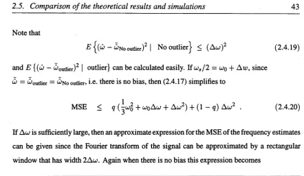
Below the threshold region the root mean squared errors (RMSE) of the frequency estimates are approximately 1000 Hz for all frequency variation A /. Above the threshold, the RMSEs of the frequency estimates of the linear FM signals which have small frequency variations are slightly greater than the RMSE of the frequency estimates when the signal has a constant frequency. On the other hand, when the frequency variation is large the RMSE is almost constant above the threshold. From Figure 2.3 it can be also observed that the threshold SNR and the RMSE above the threshold increase when the frequency variation increases.

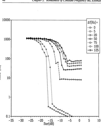
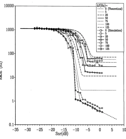
As is pointed out in [6] for constant frequency signals, an increase in the data length causes a decrease in the threshold SNR. This is also valid for linear FM signals as can be understood by comparing Figure 2.3 and the simulation results of Figure 2.4 where the simulation and the theoretical results are plotted. In Figure 2.4 the data size N is equal to the DFT size M which is 256. Another interesting point that can be observed by the comparison of the simulation results in Figure 2.3 and 2.4 is that the signal length is important for the RMSE value when the frequency variation A / is quite small. For example when A / is equal to 20 Hz, the RMSE of the frequency estimates is almost constant above threshold when N — M = 1024 whereas it is very close to the Cramer-Rao bound when N' = M = 256. This dependence of the RMSE for small values of the frequency variation A / can be better understood by Figure 2.5. As can be seen from this figure, when the frequency variation A / is relatively small the maximum peaks of the absolute value of the DFT of the signal move to the edges of the rectangular window [/o, /o + 2 A /]. However for large values of A / the location of these peaks do not change very much.

2.5. Comparison o f the theoretical results and simulations 45

similar argument is valid for the bound given for the MSE of the frequency estimates in (2.4.20). Also, this bound gets better for the signals which have larger data sizes since the peaks of the absolute value of the discrete-time Fourier transform of a signal with a fixed A / get closer to / 0 and (/o + 2A / ) as the data size increases. (See Figure 2.5.)

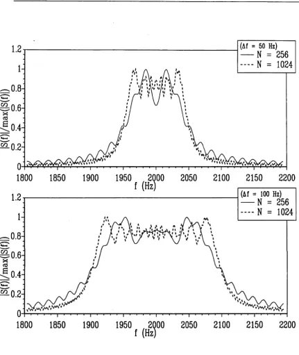
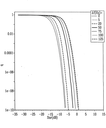
Another difference between the theoretical and simulation curves is the threshold SNRs. In order to understand this, consider the outlier probability of the frequency estimates at different SNRs and different chirp rates (Figure 2.6). Around the threshold SNR the outlier probability is very small, for example when A / = 0 Hz the outlier probability is approximately 10-6 (see Figure 2.6). Thus around one million realizations of the measurement signal have to be implemented just to observe one outlier. Since due to the computational limitations only 1000 realizations were implemented, the threshold SNRs of the simulation curves are expected to be smaller than the threshold SNRs of the theoretical curves. This also shows that simulations are impractical for finding the threshold SNRs accurately.

The increase of the RMSE (above the threshold) with an increase in the frequency variation is actually to be expected. Neglecting outliers, as we have agreed already, when we want to estimate fo + A /, the algorithm is likely to pick a frequency which is close to /o or /o + 2 A / as the maximum (this being the approximate location of the maxima of [£ (/)(). Thus this error is likely to be A /, even at very high SNR. Doubling of A / doubles the root mean squared error of the frequency estimates if the frequency variation is sufficiently large. This can be observed in the simulations for the signals which have sufficiently large frequency variations.

The probability of occurrence of outliers is primarily influenced by the height of max / | S( f ) \ above a notional noise floor, i.e. [max/ \S(f)\]/{cr2/ N). Thus if A / is doubled, so that m ax/ |5 ( / ) | is reduced by y/2, one would expect the threshold to occur at an SNR which is

\ f l

higher. Put another way, we should have a relation of the form

SNR threshold in dB = 10 lo g ( \/A /) + constant (2.5.1)

relation to hold when A / is very small. For N = 256, this relation holds for A / > 15 Hz. The constant in (2.5.1) clearly depends on the value of the data length N . However, this dependence is highly nonlinear and it is also related to the problem of finding the “optimal” data length for the ML constant frequency estimators. As shown in [2], the performance of a ML constant frequency estimator gets better as the data length increases if the signal has a constant frequency. However, if the signal is a linear FM signal with a constant chirp rate then the frequency variation increases as the data length increases. Hence there is a trade-off between the asymptotic properties and the robustness of the ML constant frequency estimator. However, finding the “optimal” data length is not a trivial process. One should be able to obtain the RMSE versus SNR curves for different data sizes as is done in Figure 2.4 where the data size N is equal to DFT size M which is 256. Afterwards by obtaining the threshold SNR versus A / curves from the RMSE versus SNR curves the dependence of the constant term in (2.5.1) on the data length can be found. Then depending on the apriori selection of the desired threshold SNR and allowable frequency variation (i.e. the degree of robustness of the estimator) it is possible to find an optimal data length from these curves.

2.6 Conclusion

In this chapter, the robustness of the ML constant frequency estimator under wrong model assumptions was investigated. The motivation for the problem was to understand the performance of the HMM-ML tandem frequency tracker where the signal is divided into time blocks and the frequency of the signal in each time block is estimated using the ML frequency estimation algorithm by assuming that the frequency of the signal is constant in those time blocks. For this purpose a linear FM signal was estimated by assuming that it had a constant frequency over the measurement time.

2.6. Conclusion ₄₇

threshold region.

Below the threshold, the RMSE for the linear FM signals was shown to be the same as the RMSE for the constant frequency case. A simple relation between the threshold SNR and the frequency variation was conjectured and supported by the theoretical curves. It was shown that the threshold SNR is a logarithmic function of the chirp rate of the linear FM signals. A discrepancy between the threshold SNRs of the simulation and the theoretical curves was observed and explained in terms of the very large number of realizations of the measurement signals required to determine the threshold region.

The work carried out in this chapter has two aspects. The first one is robustness of the maximum-likelihood constant frequency estimators with respect to model errors in general. It has been shown that there is a trade-off between the robustness and the asymptotic behaviour of these estimators. The other aspect of this work is the performance of these estimators in the framework of the HMM-ML tandem frequency trackers where the frequency of a signal is tracked by dividing the signal into segments and the frequency of each signal segment is estimated using a ML constant frequency estimator. This analysis shows that the performances of ML constant frequency estimators depend on the deviation from the model assumptions. In [1], the transitions between the frequency estimates of the signal segments are modelled using a HMM. However, even though the ML constant frequency estimators may give bad frequency estimates, the HMM part of the tandem tracker may compensate these estimates depending on the performance of the ML estimators in the other signal windows. In particular, finding the overall threshold behaviour of the HMM-ML tandem frequency tracker is an important open problem. The extension of this performance test to the HMM-ML tandem frequency trackers is an interesting research area.

Finally, in this chapter, we have concentrated on the performance of the ML constant fre­ quency estimators when they are used to estimate the frequencies of signals whose frequencies change linearly during the measurement intervals. It would be of interest to extend this work to other signals, the instantaneous frequencies of which change polynomially or randomly. In the next chapter, some other frequency variations like random walk and autoregressive frequency variations will be used to analyse the performance of the HMM-ML frequency tracker.

ESI

w

c

n

ZB

oz

10000

1000

-100

-10

-

1-0 . 1 - K

-35

^ o o o o R-o-e-o

& e e ■ & q. 0000-G-0-©

Snr(dB)

Af(Hz)=

-o- 0

5

- © -

20

- © -

50

75

100

125

5

10

2.6. Conclusion

₄₉

Af(Hz)=

--- 0 (Theoretical) ---20

--- 125

- O - 0 (Simulation) - O - 5

- e - 20 --G - 75 100

fll° O O u o

Snr(dB)

|S

(f

)|

/m

ax

(|

S

(f

)|

)

|S

(f

)|

/m

ax

(|

S

(f

)|

)

(Af = 50 Hz)

N = 256

— N =

(Af = 100 Hz)

N = 256

— N =

2.6. Conclusion

₅₁

— - 125

0

0001

le0 6

-le -0 8

-35

-30

-25

-20

-15

-10

-5

Snr(dB)

Figure 2.6: Outlier probabilities of the linear FM signals for different chirp rates when the data size N = 256, the DFT size M = 256, the sampling frequency f s = 4000 Hz, the mean frequency

References ₅₃

References

[1] A. Walker, “On the estimation of a harmonic component in a time series with stationary independent residuals,” Biometrika, vol. 58, no. 1, p. 21, 1971.

[2] E. J. Hannan, “The Estimation of Frequency,” Journal o f Applied Probability, vol. 10, pp. 510-519, 1971.

[3] T. Hasan, “Nonlinear time-series regression for a class of amplitude modulated cosinusoids,” Journal o f Time Series Analysis, no. 3, pp. 109-122,1982.

[4] R. L. Streit and R. Barrett, “Frequency Line Tracking Using Hidden Markov Models,” IEEE Transactions ASSP, vol. 38, no. 4, pp. 586-598, 1990.

[5] J. S. Rice and M. Rosenblatt, “On frequency estimation,” Biometrika, vol. 7, pp. 524-525, July 1971.

[6] D. C. Rife and R. R. Boorstyn, “Single-tone parameter estimation from discrete-time observations,” IEEE Transactions on Information Theory, vol. IT-20, no. 5, pp. 591-598, 1974.

[7] B. James, B. D. O. Anderson, and R. C. Williamson, “Characterization of Threshold for Single Tone Maximum Likelihood Frequency Estimation,” to be published in IEEE Transactions on Signal Processing, 1991.

[8] R M. Woodward, Probability and Information Theory, with Applications to Radar. Perga­ mon Press Ltd, 1953.

[9] B. G. Quinn and P. J. Kootsookos, “Threshold Behavior of the Maximum Likelihood Estimator of Frequency,” IEEE Transactions on Signal Processing, vol. 42, no. 11, pp. 3291— 3294, 1994.

[10] P. J. Parker and B. D. O. Anderson, “Frequency tracking of nonsinusoidal periodic signals in noise,” Signal Processing, vol. 20, pp. 127-152, 1990.

[11] B. Boashash, “Estimating and Interpreting the Instantaneous Frequency — Part 1: Funda­ mentals,” Proceedings o f the IEEE, vol. 80, no. 4, pp. 520-538, 1992.

[13] N. L. Johnson and S. Kotz, Continuous Univariate Distributions-2. John Wiley & Sons, 1972.

Chapter 3

Performance of HMM-ML Frequency

Trackers

3.1 Introduction

r Jn he need to estimate the frequency of a sinusoidal signal in a noisy environment arises in several areas, for example in sonar, radar etc. This problem has generated considerable interest in signal processing and statistics (e.g. [1],[2] and [3]). The techniques for the solution of this problem require that the frequency of the signal is constant during the measurement interval. However, in practical situations the frequency of the signal may change slowly with time. If this is the case, one needs to track the frequency of the signal.

There have been several approaches to track the frequency of a noisy sinusoidal signal when the signal frequency is time-varying. One approach is to use an extended Kalman filter (EKF) where a Kalman filter is used to estimate the parameters of the signal (i.e. the frequency and the amplitude) by linearizing the measurement signal around the predicted values of the signal parameters [4]. If the amplitude of the signal is known, a phase-locked loop (PLL) can also be used to track the frequency of the signal.

Another class of methods is to divide the measurement signal into finite length blocks and then use a technique to estimate the frequency of the signal in each block assuming that it is constant. In other words, the variation in the signal frequency during the measurement interval is assumed to be piecewise-continuous. La Scala and Bitmead [5] used this approach where they divided the measurement signal into finite length blocks and used an EKF to process the variation

in the Fourier coefficients of the signal in each block. They achieved tracking of the frequency of the signal at low signal to noise ratio (SNR) levels. However, one needs to be careful to tune the EKF parameters like the noise variance to take into account the extra error terms which arise during the linearization process of the signal.

A technique similar to La Scala and Bitmead’s technique was given by Streit and Barrett [6] where they divided the signal into finite length blocks and then used a hidden Markov model (HMM) filter on the maximum-likelihood estimates of the frequencies of the signals in between each block. They also assumed that the change in the frequency of the signal is piecewise- continuous, so that the signal frequency in each block was constant. Another assumption that they made was that the value of the frequency of the signal in each block depends only on the signal frequency in the previous block. In other words, they assumed that the frequencies of the signals in each block form a first order Markov chain state sequence, with finitely many states if the frequencies of the signals in each block take finitely many values. Noting that the true signal frequencies in each block are “hidden” in their ML estimates, they used a HMM Viterbi state sequence estimator to process the ML signal frequency estimates which form an output sequence of a hidden Markov model. Later Barrett and Holds worth [7] used the amplitude and the phase information to extend the results in [6]. In [8, 9], Xie and Evans used hidden Markov models for multiple frequency line tracking. Here, in the chapter, we consider the performance of the HMM-ML tandem frequency tracker given in [6].

When Streit and Barrett [6] implemented their algorithm, they divided the frequency axis into “cells”, and instead of tracking the signal frequency they tracked the cell in which the signal frequency lies. In this way, they were able to use finite state, finite output symbol HMMs (whose formulation will be explained in the next section) to model the variation in the signal frequency. Also, instead of looking at the whole range of frequency axis, they used a window which spans only a part of the frequency axis and whose location is selected with respect to the prior information on the signal frequency. Adding an extra state to the HMM to model whether the signal frequency is inside or outside of the window, they were able to reduce the computational cost of their algorithm. However, using a frequency window to track the signal frequency makes a theoretical analysis difficult to be carried out even though it reduces the computational cost. Hence, in this chapter, we assume that the whole frequency axis is used to track the signal frequency.

3.1. Introduction 57

axis is divided into cells and the cell in which the signal frequency lies is tracked. A way of doing this is to use only the coarse search part of the constant frequency estimation scheme of Rife and Boorstyn [3] explained in the previous chapter. Assume that the signal length in each block is N and a M-point DFT is used to sample the periodogram of the signal in each block (M > N ). The coarse search part of the constant frequency estimation scheme of Rife and Boorstyn can be implemented by finding the frequency bin which maximizes the absolute value of the DFT of the signal in each block. Therefore the “coarse” ML estimates of the signal frequencies can take only M different values which are uniformly distributed on the frequency axis [0, f s) where f s is the sampling frequency. Hence the frequency cells are given by [(* - 1)/S/M , i f s/ M ) for i = 1,2

When the noise level is high, i.e. SNR is low, the maximizer of the absolute value of the DFT of the signal in each block may be other than the true frequency bin. In this case, this frequency estimate is called an “outlier”. If the frequencies of the signals in each block are the states of a Markov chain which can take M different values, then these frequencies are “hidden” in the coarse ML frequency estimates.

changes in between the signal blocks as a random walk. The results of more simulation studies will also be given when the HMM-ML frequency tracker is used to track the frequency of a signal whose frequency changes as a first order auto-regressive AR(1) process. Specifically, the relation between the MSE of the estimated frequency tracks and the SNR levels and the “rate” of the stochastic frequency variations will be considered with a particular emphasis on the behaviour of the threshold SNR with respect to the signal block length and the parameters of the stochastic frequency variation.

3.2

A formulation of hidden Markov models

A detailed formulation of HMMs will be given in the Chapter 7. Nevertheless, in this section we give a formulation of HMMs which is used in this chapter to describe the HMM-ML frequency tracker.

In the context of this thesis, a hidden Markov model (HMM), or more precisely a hidden Markov Chain (HMC), is a finitely-valued stochastic process which is either a probabilistic or a deterministic function of a Markov chain. A HMM is defined in terms of two sets, each which has a finite number of elements; namely, an output set O = { 1 , 2 , . . . , M ) and a state set

S = { 1 , 2 , . . . , A}. The state of a HMM X[l] at time / takes values in the state set S. The output symbol Y[l] of the HMM is a function of the state X[l] and it takes values in the output set Ö. In this thesis, we consider discrete-time HMMs, therefore the time index l takes integer values.

When the outputs of a HMM are probabilistic functions of the states, a HMM can be defined in terms of certain real parameters A;v,m = (A, B, II). Here, A — [a,j]jvxAT is the state probability transition matrix defined by

an = P r { x [ / + l ] = j I X[/] = » }, (3.2.1)

and B = [bij]\iXN is the output probability matrix where

t>„ = Pr{y[Z] = iI = ,

i = 1 , . . . , M and j = 1 , . . . , N, V / (3.2.2)